Lists in a Lighthouse

(1)

University of South Carolina

Scholar Commons

Theses and Dissertations

2015

Neutrino and Antineutrino Induced Meson

Production

Libo Jiang

University of South Carolina

Follow this and additional works at:https://scholarcommons.sc.edu/etd Part of thePhysics Commons

This Open Access Dissertation is brought to you by Scholar Commons. It has been accepted for inclusion in Theses and Dissertations by an authorized administrator of Scholar Commons. For more information, please [email protected].

Recommended Citation

(2)

Neutrino and Antineutrino Induced Meson Production

by

Libo Jiang

Bachelor of Science

Northeast Forest University 2006 Master of Science

Harbin Institute of Technology 2008

Submitted in Partial Fulfillment of the Requirements for the Degree of Doctor of Philosophy in

Physics

College of Arts and Sciences University of South Carolina

2015 Accepted by:

Roberto Petti, Major Professor Vitaly Rassolov, Committee Member

Steffen Strauch, Committee Member Jeffery Wilson, Committee Member

(3)

c

(4)

Dedication

(5)

Acknowledgments

First of all, great gratitude to Professor Roberto Petti and Professor Sanjib Mishra. They gave me indispensable guidance and assistance to my work during the past few years and let me know how beautiful the physics is. 5 years ago, they warmly brought me into neutrino physics area, and are very thoughtful and helpful in supervision of my research and schedule. They continued answering my queries endlessly.

Many thanks to my committee members, Dr. Vitaly Rassolov, Dr. Steffen Strauch, and Dr. Jeff Wilson. Their guidance and help are very important to my research.

Many thanks to my colleagues and friends at University of South Carolina: Xinch--un Tian, Chris Kullenberg, Brian Mecurio, Jae Jun Kim, Kevin Wilson, Hongyue Duyang, Andrew Svenson, Kevin Wood, Tyler Alion, and Bing Guo. During the past few years, they gave me a lot of help and I had the pleasure of working with them.

I would also like to say a few works to thank Dr. Huifeng Fu, and Dr. Tian-hong Wang. They helped a lot in my theoretical calculations and understanding the electroweak theory.

Thank to the excellent work of the collaborators from ELBNF/DUNE, NOMAD collaborations.

(6)

Abstract

Coherent meson production measurement is very important in physics research. First, the coherent pion production is a potential background to ν oscillation in next gen-eration of Long Base Line Experiment(ELBNF/DUNE); second, coherent pion and coherentρproduction provide a detailed test of CVC and PCAC hypothesis; third, co-herent meson production can be used to monitor the neutrino and anti-neutrino fluxes in the experiment. This dissertation focuses on two parts: coherentπ− production in

NOMAD, and coherentρsimulation using LBNF fluxes. With the NOMAD data, the ratio between cross-sections of coherent π− and ¯_ν

µ charged current interactions was

measured and compared with the measurements of coherent π+. The experience of coherentπanalysis may be used to evaluate the sensitivity of ELBNF/DUNE project to coherent processes. With the ELBNF process, I wrote a new C++ simulation pack-age and generated 100k coherentρ+ events. It is known that for the neutrino-induced process, the incoming neutrino fluxes could not be measured directly, and theQ2 and other variables related to it are unknown in the neutrino-induced neutral current interactions. The photon-induced coherent ρ0 provides a way to get additional in-formation to constrain the incoming neutrino fluxes. I calculated the ratios between the cross-sections of neutrino-induced coherent ρ±, _ρ0 and photon-induced coherent

ρ0. With these ratios, some kinematic variable distributions are reweighted with this

(7)

List of Tables

Table 3.1 Table of vector and axial vector couplings. . . 47

Table 5.1 Summary of performance for the fine grained tracker configuration [1]. 59 Table 5.2 Parameters for the fine-grained tracker [1]. . . 63

Table 5.3 Parameters of the UA1/NOMAD dipole magnet [18]. . . 69

Table 6.1 Normalization of Neutrino Beam Mode events [52, 8]. . . 80

Table 6.2 Ratios between interaction mode. . . 80

Table 6.3 Minimum value for the fiducial volume in NOMAD. . . 81

Table 6.4 Cut table of Monte Carlo events in generated level. . . 83

Table 6.5 Reconstructed variable cut table after normalization and reweighted. 84 Table 6.6 The efficiency (ratio between Reconstructed ¯νµ CC and Simu-lated ¯νµ CC events) in 7 Eν bins. . . 90

Table 6.7 Reconstructed ¯νµCC events without normalization with the fac-tor from fit. . . 91

Table 6.8 Raw signal and fully corrected data after normalization. . . 91

Table 6.9 Fully corrected signal got from efficiency vector (shown in Table 6.6). 92 Table 6.10 ¯νµ CC events as a function of Eν (Evis) before normalization with the factor got from fit. . . 93

Table 6.11 ¯νµ CC efficiency matrix. . . 93

(11)

Table 6.13 Fully corrected signal got from efficiency matrix. . . 95

Table 6.14 Normalization of the MC events. . . 101

Table 6.15 Summary of event reduction in different data and MC samples

for the preselection cuts. . . 102

Table 6.16 The NN cut table (the beam(flux) reweight is applied to all the ¯

νµ-CC events). . . 116

Table 6.17 Kinematic information of a coherent π− event corresponding to

Figure 6.36 survived from preselection and Neural Network. . . 118

Table 6.18 BN and SN table in 7 visible energy (Evis) bins, calculated from variable BN depends on the Evis(R=σ(Cohπ−₎

σ(¯νµCC)). . . 119 Table 6.19 BN and SN table in 7 visible energy (Evis) bins, using a fixed

BN(R=σ(Cohπ−₎

σ(¯νµCC)). . . 120 Table 6.20 Signal in signal region, and Generated signal information

calcu-lated from variable BN. . . 121

Table 6.21 Norm-bkg, Corr-sig as a function of Evis in 7 bins calculated

from variable BN. . . 122

Table 6.22 Corrected signal (Corr-Sig) as a function of Evis in 7 bins cal-culated from variable BN(R=σ(Cohπ−₎

σ(¯νµCC)). . . 123 Table 6.23 Corrected signal (Corr-Sig-Enus) as a function of Eν in 7 bins

calculated from variable BN(R=σ(Cohπ−₎

σ(¯νµCC)). . . 126 Table 6.24 Norm-bkg, Corr-sig as a function of Evis in 7 bins, calculated

from a fixed BN. . . 127

Table 6.25 Corrected signal (Corr-sig) as a function of Evis in 7 bins, cal-culated from a fixed BN(R=σ(Cohπ−₎

σ(¯νµCC)). . . 128 Table 6.26 Corrected signal (Corr-sig) as a function of Eν in 7 bins

calcu-lated from a fixed BN(R=σ(Cohπ−₎

σ(¯νµCC) ). . . 128 Table 6.27 Normalization of (Anti-)Neutrino Beam Mode events [8]. . . 131

(12)

Table 6.29 Cut table of Monte Carlo events in generated level. . . 132

Table 6.30 Reconstructed variable cut table after normalization and reweighted. 133

Table 6.31 Reconstructed ¯νµ charged current events without normalization. . 136

Table 6.33 The efficiency (ratio between Rec-¯νµ CC and Gen-¯νµCC events)

in 7 Eν bins. . . 137

Table 6.34 Fully corrected signal get from efficiency vector (shown in Table 6.33).137

Table 6.35 ¯νµ charged current events as a function of Eν (Evis) before

nor-malization. . . 138

Table 6.36 Background as a function of Eν and Evis before normalization. . . 138

Table 6.38 Fully corrected signal get from efficiency matrix. . . 140

Table 6.39 Normalization of the MC events. . . 140

Table 6.40 Summary of event reduction in different data and MC samples

for the preselection cuts. . . 141

Table 6.41 The NN cut table (the beam(flux) reweight is applied to all the ¯

νµ-CC and νµ-CC events). . . 156

Table 6.42 Kinematic information of a coherent π− event corresponding to

Figure 6.68 survived from preselection and Neural Network. . . 158

Table 6.43 BN and SN table in 7 Bins, calculated from variable BN depends on the Evis(R=σ(Cohπ−₎

σ(¯νµCC)). . . 159

Table 6.44 BN, and δBN table, using a fixed BN(R=σ(Cohπ −₎

σ(¯νµCC)). . . 159 Table 6.45 Signal in signal region, and Generated signal information

calcu-lated from variable BN. . . 159

Table 6.46 Norm-bkg, Corr-sig as a function of Evis in 7 bins calculated

(13)

Table 6.47 Corrected signal (Corr-Sig) as a function of Evis in 7 bins cal-culated from variable BN(R=σ(Cohπ−₎

σ(¯νµCC)). . . 162

Table 6.48 Corrected signal (Corr-Sig-Enus) as a function of Eν in 7 bins calculated from variable BN(R=σ(Cohπ−₎ σ(¯νµCC)). . . 162

Table 6.49 Norm-bkg, Corr-sig as a function of Evis in 7 bins, calculated from a fixed BN. . . 165

Table 6.50 Corrected signal (Corr-sig) as a function of Evis in 7 bins, cal-culated from a fixed BN(R=σ(Cohπ−₎ σ(¯νµCC)). . . 166

Table 6.51 Corrected signal (Corr-Sig-Enus) as a function of Eν in 7 bins, calculated from a fixed BN(R=σ(Cohπ−₎ σ(¯νµCC) ). . . 166

Table 6.52 Comparison of R=σ(Cohπ−₎ σ(¯νµCC) :FocP and R= σ(Cohπ−₎ σ(¯νµCC) :FocN as a func-tion of Evis using variable BN.) . . . 169

Table 6.53 Comparison of R=σ(Cohπ−₎ σ(¯νµCC) :FocP and R= σ(Cohπ−₎ σ(¯νµCC) :FocN as a func-tion of Eν using variable BN. . . 169

Table 6.54 Comparison of R=σ(Cohπ−₎ σ(¯νµCC) and R= σ(Cohπ+₎ σ(νµCC) as a function of Evis using variable BN. . . 172

Table 6.55 Comparison of R=σ(Cohπ−₎ σ(¯νµCC) and = σ(Cohπ+₎ σ(νµCC) as a function of Eν using variable BN. . . 175

Table 6.56 Comparison of R=σ(Cohπ−₎ σ(¯νµCC):FocP and R= σ(Cohπ−₎ σ(¯νµCC):FocN calcu-lated from a fixed BN. . . 180

Table 6.57 Comparison of R=σ(Cohπ−₎ σ(¯νµCC) and R= σ(Cohπ+₎ σ(νµCC) calculated from a fixed BN. . . 180

Table 6.58 Comparison between different background subtractions. . . 182

Table 6.59 Smearing matrix of Cohπ−:FocP . . . 183

Table 6.60 Smearing matrix of Cohπ−:FocN . . . 183

(14)

Table 6.62 Final state interaction (FSI) error as a function of energy in 14

bins . . . 185

Table 6.63 BN and SN table in 7 Bins using variable BN depends on the

Evis in 7 bins. . . 186

Table 6.64 BN and SN table in 7 Bins using a fixed BN. . . 186

Table 6.65 Norm-bkg, Corr-sig as a function of Evis in 7 bins using variable BN.187

Table 6.66 Corrected signal (Corr-Sig) as a function of Evis in 7 bins using

variable BN. . . 188

Table 6.67 Corrected signal (Corr-Sig-Enus) as a function of Eν in 7 bins

using variable BN. . . 188

Table 6.68 Norm-bkg, Corr-sig as a function of Evis in 7 bins using a fixed BN(the the beam(flux) reweight is applied to both of the ¯νµ-CC

events andνµ-CC events). . . 189

Table 6.69 Corrected signal (Corr-Sig) as a function of Evis in 7 bins using

a fixed BN. . . 190

using a fixed BN. . . 190

Table 6.71 BN and SN table in 7 Bins using variable BN depends on the

Evis in 7 bins. . . 191

Table 6.72 BN and SN table in 7 Bins using a fixed BN. . . 191

Table 6.73 Norm-bkg, Corr-sig as a function of Evis in 7 bins using variable BN.192

Table 6.74 Corrected signal (Corr-sig) as a function of Evis in 7 bins using

variable BN. . . 193

Table 6.76 Norm-bkg, Corr-sig as a function of Evis in 7 bins using a fixed BN. 194

Table 6.77 Corrected signal (Corr-sig) as a function of Evis in 7 bins using

(15)

using a fixed BN. . . 195

Table 6.79 Comparison between RS and BS signal model simulation. . . 196

Table 6.80 Systematic on signal modeling. . . 197

Table 6.81 Comparison of R=σ(Cohπ−₎

σ(¯νµCC) :FocP and R=

σ(Cohπ−₎

σ(¯νµCC) :FocN as a

func-tion of Evis using variable BN. . . 198

σ(Cohπ−₎

func-tion of Eν using variable BN. . . 198

σ(Cohπ−₎

func-tion of Evis calculated from a fixed BN. . . 198

σ(Cohπ−₎

func-tion of Eν calculated from a fixed BN. . . 203

Table 6.85 Ratio between R=σ(Cohπ−₎

σ(¯νµCC) and R=

σ(Cohπ+₎

σ(νµCC) as a function of Eν

Table 6.86 Ratio between R=σ(Cohπ−₎

σ(Cohπ+₎

calculated from a fixed BN. . . 203

Table 6.87 Variation of Selection Cuts. . . 204

Table 6.88 The error of cross-section of charged current resonance and

co-herent ρ events in 14 bins. . . 206

Table 6.89 Summary of experimental measurements of coherentπ−

(16)

List of Figures

Figure 1.1 The (Q2,ν) plane in neutrino interactions [36]. . . 2

Figure 1.2 Diagrams of Weak Charged and Neutral Current . . . 9

Figure 1.3 Total cross-section as a function of energy for interactions of

photons and hadrons [50]. . . 14

Figure 2.1 The significance with which the mass hierarchy (top) and CP violation (δCP 6= 0 or π, bottom) can be determined by the

LBNE experiment with 34-kt far detector as a function of the value ofδCP. The plots on the left are for normal hierarchy and

the plots on the right are for inverted hierarchy. The width of the red band shows the range of the sensitivity that is achieved by LBNE when varying the beam design and the signal and

background uncertainties [1] . . . 16

Figure 2.2 Normal and inverted mass hierarchy [35]. . . 18

Figure 2.3 The expected reconstructed neutrino energy spectrum of νµ or

¯

νµ events in a 34-kt LArTPC for three years of neutrino(left)

and anti-neutrino(right) running with a 1.2-MW beam [1]. . . 19

Figure 2.4 The expected reconstructed neutrino energy spectrum of νe or

¯

νe oscillation events in a 34-kt LArTPC for three years of

neu-trino (left) and anti-neuneu-trino (right) running with a 1.2-MW, 80-GeV beam assuming sin2₍₂₍₂_θ

13) = 0.09. The plots on the top are for normal hierarchy and the plots on the bottom are

for inverted hierarchy [1]. . . 20

Figure 2.5 The mass hierarchy (left) and CP violation (right) sensitivities as a function of exposure in kt· year, for true normal hierar-chy. The band represents the range of signal and background

normalization errors [1]. . . 21

(17)

Figure 2.7 νe and ¯νeflux distribution in ELBNF/DUNE project. . . 24

Figure 3.1 Kinematics of neutrino scattering. . . 27

Figure 4.1 Predicted neutrino(νµ) and anti-neutrino (¯νµ)flux in NOMAD. . . 50

Figure 4.2 Schematic layout of the West Area Neutrino Facility(WANF) beam line [8]. . . 50

Figure 4.3 Diagram of the NOMAD detector (top view) [5] . . . 52

Figure 4.4 νµ-CC candidates in NOMAD. . . 54

Figure 4.5 ¯νe-CC candidates in NOMAD. . . 54

Figure 4.6 QE candidates in NOMAD. . . 55

Figure 4.7 Resonance candidates in NOMAD. . . 55

Figure 4.8 Coherent ρ0 candidate event picture. . . 56

Figure 4.9 Coherent π+ candidate event picture. . . 56

Figure 4.10 Coherent π− candidate event picture. . . 57

Figure 5.1 Sketch of the proposed HIRESMNU detector showing the inner STT and the 4π ECAL in the dipole magnet with the muon-ID detector(MRD). The internal magnetic volume is approxi-mately 4.5m×4.5m×8m. Also shown is one module of the pro-posed STT [18] . . . 61

Figure 5.2 Layout of the straw layers and cross-section of an STT Module [18]. 63 Figure 5.3 Sketch of a basis STT module for the measurement of nuclear effects. Several modules can be placed in the upstream magnetic volume with different target materials(Pb,Fe etc.) of the same thickness in radiation length [18]. . . 64

Figure 5.4 Schematic of the ATLAS STT Endplug [18]. . . 65

(18)

Figure 5.6 DownStream(DS) or Forward ECAL [18]. . . 67

Figure 5.7 Specifications of the Barrel ECAL [18]. . . 68

Figure 5.8 UpStream(UP) ECAL [18]. . . 68

Figure 5.9 Specs of the UA1/NOMAD dipole magnetic [18]. . . 70

Figure 5.10 Conceptual sketch of one of the C-sections that constitute the magnet return yoke (dimensions are in mm). The vertical di-mension is longer that the horizontal one in order to accommo-date the magnet coil [18]. . . 71

Figure 5.11 Cross-section of a Resistive Plate Chamber with its associated strips for the read out of the induced signal [18]. . . 72

Figure 5.12 Layout of the HIRESMNU with downstream, external muon-ID detector(EMI) and shielding. The EMI specifications are pre-liminary; detailed simulation studies of EMI will yield a more robust design [18]. . . 73

Figure 5.13 Momentum and Energy resolution of HIRESMNU [18]. . . 73

Figure 6.1 Feynman Diagram of Coherent Pion Production. . . 75

Figure 6.2 Principle of the focusing. The lines are representative trajecto-ries of particles of three different momenta [8]. . . 77

Figure 6.3 Distribution of the angle between theπ+momentum vector and the beam line direction,PT/P, just upstream of the horn (top left),right after it(top right) and the ratio of the latter to the former(bottom) [8]. . . 78

Figure 6.4 Distribution of the angle between theπ−momentum vector and the beam line direction,PT/P, just upstream of the horn (top left),right after it(top right) and the ratio of the latter to the former(bottom) [8]. . . 79

Figure 6.5 Reconstruction of the event kinematics for individual events. . . . 82

(19)

Figure 6.7 χ2distribution with respect tokN C

norm, fixknormν¯µCC = 0.961,knormνµCC =

1.445 using 125 points. . . 88

Figure 6.8 χ2distribution with respect tokνµCC

norm, fixknormν¯µCC = 0.961,knormN C =

2.052 using 125 points. . . 89

Figure 6.9 An example of the structure of an artificial neutral network [21]. . 96

Figure 6.10 Pm

T distribution of the neutrino beam mode data (positive

fo-cusing data: FocP). . . 97

Figure 6.11 Xbj distribution of the neutrino beam mode data (positive

fo-cusing data: FocP). . . 98

Figure 6.12 ζ distribution of the neutrino beam mode data (positive

focus-ing data: FocP). . . 98

Figure 6.13 The NN distribution comparison of background and signal. . . 99

Figure 6.14 The NN distribution comparison of Data and MC. . . 99

Figure 6.15 The distribution of sensitivity of the neural network in coherent

π− analysis of neutrino beam mode. . . 103

Figure 6.16 The Ybj distribution from different contributions, ν-CC, ¯ν-CC,

NC, ¯ν-Cohρ− and Coh_π− in _{background (control) region} and

the Comparison between Data (points with error bars) and

MC(histogram). . . 106

NC, ¯ν-Cohρ− and Coh_π− in_{signal (>0.7) region} and the

Com-parison between Data (points with error bars) and MC(histogram). 106

Figure 6.18 TheXbj distribution from different contributions, ν-CC, ¯ν-CC,

(20)

Figure 6.20 The ζπ distribution from different contributions, ν-CC, ¯ν-CC,

NC, ¯ν-Cohρ− and Coh_π− in

signal (>0.7) region and the

Figure 6.22 The Q2 distribution from different contributions, ν-CC, ¯ν-CC, NC, ¯ν-Cohρ− and Coh_π− in _{background (control) region} and

Figure 6.23 The Q2 distribution from different contributions, ν-CC, ¯ν-CC, NC, ¯ν-Cohρ− and Cohπ− insignal (>0.7) region and the

Figure 6.24 ThePTm distribution from different contributions,ν-CC, ¯ν-CC,

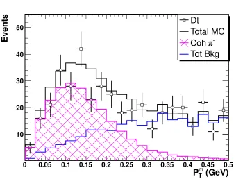
Figure 6.25 ThePm

T distribution from different contributions,ν-CC, ¯ν-CC,

Figure 6.26 The t distribution from different contributions, ν-CC, ¯ν-CC, NC, ¯ν-Cohρ− and Coh_π− in _{background (control) region} and

Figure 6.27 The t distribution from different contributions, ν-CC, ¯ν-CC, NC, ¯ν-Cohρ− and Coh_π− in_{signal (>0.7) region} and the

Figure 6.28 The t0 distribution from different contributions, _ν-CC, ¯_ν-CC,

(21)

Figure 6.30 The Eπ distribution from different contributions, ν-CC, ¯ν-CC,

Figure 6.32 The ΦP T

had distribution from different contributions, ν-CC, ¯ν

-CC, NC, ¯ν-Cohρ− and Coh_π− in _{background (control) region}

and the Comparison between Data (points with error bars) and

haddistribution from different contributions,ν-CC, ¯ν-CC,

NC, ¯ν-Cohρ− and Cohπ− insignal (>0.7) region and the

Figure 6.34 The angleθ between Muon and Pion distribution from differ-ent contributions, ν-CC, ¯ν-CC, NC, ¯ν-Cohρ− and Coh_π− in

background (control) region and the Comparison between Data

(points with error bars) and MC(histogram). . . 115

Figure 6.35 The angle θ distribution from different contributions, ν-CC, ¯

ν-CC, NC, ¯ν-Cohρ− and Coh_π− in _{signal (>0.7) region} and

Figure 6.36 Coherent π− event picture originated by ¯_ν

µ contamination in

the neutrino mode. . . 117

Figure 6.37 The distribution of BN as a function of visible energy (Evis) in

7 bins(the beam(flux) reweight is applied to all the ¯νµ-CC events). 120

Figure 6.38 R=σ(Cohπ−₎

σ(¯νµCC) distribution in both linear scale (top) and log scale (bottom), calculated using a variable BN which depends on the

Evis(the beam(flux) reweight is applied to all the ¯νµ-CC events). . 124

Figure 6.39 R×<E> distribution in both linear scale (top) and log scale (bottom), calculated using a variable BN which depends on the

(22)

σ(¯νµCC) distribution in both linear scale (top) and log scale (bottom), calculated from a fixed BN (the beam(flux) reweight

is applied to all the ¯νµ-CC events). . . 129

Figure 6.41 R×<E> distribution in both linear scale (top) and log scale (bottom), calculated from a fixed BN (the beam(flux) reweight

Figure 6.42 Pm

T distribution of the anti-neutrino beam mode data (negative

focusing data: FocN). . . 142

Figure 6.43 Xbj distribution of the anti-neutrino beam mode data (negative

Figure 6.44 ζ distribution of the anti-neutrino beam mode data (negative

Figure 6.45 The NN distribution comparison of background and signal. . . 144

Figure 6.46 The NN distribution comparison of Data and MC. . . 144

Figure 6.47 The distribution of sensitivity of the neural network in coherent

π− analysis of anti-neutrino beam mode. . . 145

the Comparison between Data (points with error bars) and MC

(histogram). . . 146

Com-parison between Data (points with error bars) and MC (histogram).146

NC, ¯ν-Cohρ−and Coh_π−in_{signal (>0.70) region}and the

(23)

Com-parison between Data points with error bars) and MC (histogram). 148

Figure 6.54 The Q2 distribution from different contributions, ν-CC, ¯ν-CC, NC, ¯ν-Cohρ− and Coh_π− in _{background (control) region} and

Figure 6.55 The Q2 distribution from different contributions, ν-CC, ¯ν-CC, NC, ¯ν-Cohρ− and Cohπ− insignal (>0.7) region and the

Figure 6.56 ThePTm distribution from different contributions,ν-CC, ¯ν-CC,

Figure 6.57 ThePm

T distribution from different contributions,ν-CC, ¯ν-CC,

Figure 6.58 The t distribution from different contributions, ν-CC, ¯ν-CC, NC, ¯ν-Cohρ− and Coh_π− in _{background (control) region} and

Figure 6.59 The t distribution from different contributions, ν-CC, ¯ν-CC, NC, ¯ν-Cohρ− and Coh_π− in_{signal (>0.7) region} and the

(24)

-CC, NC, ¯ν-Cohρ− and Coh_π− in _{background (control) region}

and the Comparison between Data (points with error bars) and

MC (histogram). . . 154

-CC, NC, ¯ν-Cohρ− and Cohπ− in signal (>0.7) region and the Comparison between Data (points with error bars) and MC

Figure 6.66 The angleθ between muon and pion distribution from differ-ent contributions, ν-CC, ¯ν-CC, NC, ¯ν-Cohρ− and Coh_π− in

background (control) region and the Comparison between Data

(points with error bars) and MC (histogram). . . 155

Figure 6.67 The angle θ distribution from different contributions, ν-CC, ¯

ν-CC, NC, ¯ν-Cohρ− and Coh_π− in _{signal (>0.7) region} and

he Comparison between Data points with error bars and MC

Figure 6.68 Coherent π− event picture originated by ¯_ν

µ contamination in

the anti-neutrino mode. . . 157

Figure 6.69 The distribution of BN as a function of visible energy(Evis) in

7 bins (the beam(flux) reweight is applied to all the ¯νµ-CC events). 160

σ(¯νµCC) distribution in both linear scale (top) and log scale (bottom), calculated from variable BN which depends on the

Evis (the beam(flux) reweight is applied to all the ¯νµ-CC events). 163

Figure 6.71 R×<E> distribution in both linear scale (top) and log scale (bottom), calculated from variable BN which depends on the

(25)

σ(¯νµCC) distribution in both linear scale (top) and log scale (bottom), calculated from a fixed BN (the beam(flux) reweight

Figure 6.73 R×<E> distribution in both linear scale (top) and log scale (bottom), calculated from a fixed BN (the beam(flux) reweight

Figure 6.74 Comparison of R=σ(Cohπ−₎

σ(¯νµCC):FocP and R=

σ(Cohπ−₎

σ(¯νµCC):FocN as a

function ofEν using variable BN. . . 170

Figure 6.75 Distribution of the sum of R=σ(Cohπ−₎

σ(Cohπ−₎ σ(¯νµCC):FocN

as a function of Eν using variable BN. . . 171

σ(Cohπ+₎

σ(νµCC) using variable BN. . . 173

σ(Cohπ+₎

σ(νµCC) using variable BN. . . 174

σ(Cohπ−₎

σ(¯νµCC):FocN

calcu-lated from a fixed BN. . . 176

Figure 6.79 Distribution of the sum of R=σ(Cohπ−₎

σ(Cohπ−₎ σ(¯νµCC):FocN

calculated from a fixed BN. . . 177

σ(Cohπ+₎

σ(νµCC) calculated from a

fixed BN. . . 178

σ(Cohπ+₎

σ(νµCC) calculated from a

fixed BN. . . 179

σ(¯νµCC) calculated from a fixed BN to R=

σ(Cohπ−₎ σ(¯νµCC) calculated from variable BN. . . 181

σ(¯νµCC) between BS and RS Model

calcu-lated from a fixed BN. . . 197

σ(Cohπ+₎

σ(νµCC) as a function ofEν

σ(Cohπ+₎

σ(νµCC) as a function ofEν

(26)

Figure 6.86 Ratio between R=σ(Cohπ−₎

σ(Cohπ+)

Figure 6.87 Ratio between of R=σ(Cohπ−₎

σ(Cohπ+₎

σ(νµCC) as a function of

Eν calculated from a fixed BN. . . 202

Figure 6.88 Total energy-dependent uncertainties on the yields of each of

the neutrino species(νµ and ¯νµ). . . 205

Figure 7.1 Feynman diagram of photon induced coherentρ process. . . 209

Figure 7.2 Q2 distribution of neutrino induced coherent ρ+ events gener-ated from LBNE flux and photon induced coherent events ob-tained fromν-induced coherent ρ+ events reweighted by factor

π2_α2

G2

FQ4. . . 214 Figure 7.3 Xbj distribution of neutrino induced coherentρ+ events

gener-ated from LBNE flux and photon induced coherent events ob-tained fromν-induced coherent ρ+ events reweighted by factor

π2_α2

G2

FQ4. . . 215 Figure 7.4 Ybj distribution of neutrino induced coherentρ+ events

π2_α2

G2

FQ4. . . 216 Figure 7.5 Pm

T distribution of neutrino induced coherent ρ+ events

π2_α2

G2

FQ4. . . 217 Figure 7.6 ζρdistribution of neutrino induced coherentρ+events generated

from LBNE flux and photon induced coherent events obtained fromν-induced coherent ρ+ events reweighted by factor π2_α2

G2

FQ4. . . 218 Figure 7.7 t distribution of neutrino induced coherentρ+ events generated

from LBNE flux and photon induced coherent events obtained fromν-induced coherent ρ+ events reweighted by factor π2_α2

G2

(27)

Chapter 1 Electroweak Theory and Neutrino Interaction

1.1 Weak Interaction and Electroweak Theory

Theoretically, all the interactions between particles can be classified into four funda-mental interactions and listed in order of decreasing strength as: the strong inter-action, electromagnetism, the weak interinter-action, and gravity. The weak interaction operates between all particles except photons and gravitons. It causes reactions which make particles ultimately decay into the stable leptons and hadrons, such as electrons, neutrinos, protons, and so on. These decays are the natural sources for us to study the weak interaction, however, only in a limited energy region. The advent of neu-trino experiments in humans’ laboratories ameliorated the situation by enabling us to explore weak interactions in a much wider energy region. The neutrino-hadron scattering is one such experiment.

The neutrino-hadron scattering can be classified with the help of a plane composed of Q2 and ν [16], where Q2 and ν are the square of the momentum transfer and the energy transfer between the initial and final leptons respectively (Q2 and ν are defined in chapter 2). Figure 1.1 shows the weak interactions with respect toQ2 and

ν. In this figure, Region I with very smallQ2 and ν represents weak decays; Region II (diagonal line) represents (quasi-)elastic scattering; Region III is the resonance region, starting with the line W =M+mπ(W is the hadronic mass, M is the proton

mass, mπ is the pion mass); Region IV with high values of Q2 and ν is the domain

(28)

scattering, which is the focus of this thesis. In this Region, the interactions with very lowQ2 allow study two basic properties of the weak current: One is the conservation of the vector current (It is also called CVC hypothesis), which was introduced to explain the equality of the vector muon and nuclear beta decay. The other one is the partial conservation of the axial current (It is also called PCAC hypothesis) which can be used to explain the small (∼20%) renormalization of the nuclear axial decay constant by the strong interactions [36]. When the Q2 is very low, the nuclear stays intact in coherent process, then the nucleons inside can not be considered as free. In this case, the perturbative theory of strong interactions can not be used. To study the processes with very low Q2, the Hadron Dominance Model has been brought up to describe the hadronic behavior in coherent process, which is going to be introduced in this chapter. Therefore, the study of coherent meson production can also provide a detailed test of Hadron Dominance Model.

Q

2(

GeV

2)

2M ν(GeV2₎

I

II

III

IV

V

x= 1 W=M+mπ

x=C

(29)

Space-Time Structure of the Weak Charged and Neutral

Current

This subsection gives basics of electroweak theory (which can be found in many textbooks, such as [33] and [30]). For convenience, we give the convention for the Dirac matrices in this thesis as follows.

Let{γµ, µ= 0,1,2,3}be an orthonormal set of vectors in space-time. The

signa-ture of space-time is expressed by the equations:

γ₀2 = 1, γ₁2 =γ₂2 =γ₃2 =₋1, (1.1)

γµ = gµνγν, (1.2)

and the matrices follow an anti-commutation relation:

{γµ, γν}+ =

1

2(γµγν +γνγµ) = gµν. (1.3)

As usual, a special multivector

iγ0γ1γ2γ3 = γ5 (1.4)

is introduced which can be used to construct peudoscalars. A multivetor is said to be even (odd) if it commutes (anti-commutes) with γ5. A slashed 4-momentum (or other 4-vector) represents the product of the 4-momentum (or other 4-vector) with

γµ.

In the Standard Model the electroweak interaction is described by a gauge field theory. The gauge group is the SU(2)L×U(1)Y group, where L indicates that this

SU(2) group only acts on the left-handed components of fermion fields. The subscript

Y for U(1) group is called hypercharge and specifies this U(1) group.

The local SU(2)L × U(1)Y gauge invariance of the electroweak Lagrangian is

guaranteed by introducing the covariant derivativeDµ,

Dµ=∂µ+igAiµτi+ig0Bµ

Y

(30)

where τi = _σi_/2 (_i = 1_,2_,3) with _σi being the Pauli matrix. _Ai

µ and Bµ are gauge

boson fields. For each generator of the group, there is a gauge field. The covariant derivative transforms as

Dµ →Dµ0 =U(θi(x), η(x))DµU−1(θi(x), η(x)), (1.6)

where

U(θi(x), η(x)) =eiθi(x)τi+iη(x)Y /2, (1.7)

with θi(_x) and _η(_x) being the parameters of the transformation. Then the gauge

boson fields transform as

Ai_µτi →A0i_µτi =U(θj(x))[Ai_µτi− i g∂µ]U

−1₍

θi(x)), (1.8)

Bµ →Bµ0 =Bµ−

1

g0∂µη(x). (1.9)

The interaction part of the Lagrangian can be written as

LI = −

1

2L¯L(g /A i

σi−g0B/)LL−

1

2Q¯L(g /A i

σi+ 1

3g0B/)QL

+g0e¯RBe/ R− 2₃g0u¯RBu/ R+1₃g0d¯RBd/ R, (1.10)

whereLLand QL represent the left-handed lepton doublet and the left-handed quark

doublet in the fundamental representation ofSU(2)Lgroup respectively. Specifically,

for the first generation of the Standard Model,

LL =

νeL

eL

!

, QL=

uL

dL

!

. (1.11)

In order to see the interaction term for neutrinos explicitly, we take the explicit form of the Pauli matrices and obtain

LI,L = −

1 2

¯ νeL eL

_  

g /A3 −g0B/ g(A/1−i /A2) g(A/1+i /A2) −g /A3−g0B/

        νeL eL    

+g0_e¯

(31)

where we have omitted the quark part of the Lagrangian. This equation shows that the interactions are inter-mediated by the mixtures of the gauge fields. The off-diagonal terms of Equation (1.12) are conjugations of each other, so we can introduce a complex fieldWµ by

Wµ≡ A

µ

1_√−iAµ2

2 . (1.13)

Replacing Aµ₁ and Aµ₂ with Wµ, we have, for interactions between neutrinos and

electrons,

L(CC) = ₋_√g

2{ν¯eLW e/ L+ ¯eLW/ †

νeL}

= −₂√g

2ν¯eγµ(1−γ5)eWµ+H.c.

= −₂√g

2jW,Lµ Wµ+H.c., (1.14)

where

jW,Lµ = ¯νeγµ(1−γ5)e = 2 ¯νeγµeL. (1.15)

The complex gauge field Wµ carries a charge which should be the electrical charge

to guarantee the conservation of electrical charge. So the current j_W,Lµ is called the (leptonic) charged current and the corresponding part of Lagrangian is indicated by CC (which represents charged current) as a superscript (see Equation (1.14)).

The diagonal terms of Equation (1.12) are mixtures of Aµ₃ and Bµ, so we can

introduce two fields Zµ and _Aµ as the linear combinations of _A

3 and Bµ by

Aµ = sinθWAµ3 + cosθWBµ, (1.16)

Zµ = cosθWAµ3 −sinθWBµ, (1.17)

whereθW is a parameter to be determined and is usually called the weak mixing angle

or Weinberg angle. Recalling that the electromagnetic interaction should come out of the electroweak theory, we require thatAµis just the photon field. This requirement

determines the Weinberg angle and the relation among the couplings g, g0 and the

(32)

To see how this happens, let us pick up the neutral current (NC) Lagrangian from Equation (1.12):

L(N C)=₋1

2{ν¯eL(g /A3−g0B/)νeL−e¯L(g /A3+g0B/)eL−2g0e¯RBe/ R}. (1.18)

Substituting Aµ₃ and Bµ with _Aµ and _Zµ by using Equations (1.16) and (1.17), we

obtain

L(N C) = ₋1

2{ν¯eL[gcosθW +g0sinθW)Z/ + (gsinθW −g0cosθW)A/]νeL

−e¯L[gcosθW −g0sinθW)Z/ + (gsinθW +g0cosθW)A/]eL

−2g0e¯R[−sinθWZ/ + cosθWA/]eR}. (1.19)

As neutral particles, neutrinos should not interact with the electromagnetic field, so we have

gsinθW =g0cosθW. (1.20)

Now taking this relation back into Equation (1.19), we obtain

L(I,LN C) = −

g

2 cosθW{ ¯

νeLZν/ eL−(1−2 sin2θW) ¯eLZe/ L+ 2 sin2θWe¯RZe/ R}

+gsinθWe /¯Ae. (1.21)

The last term describes electrons interacting with photons, which is just what we need for electromagnetic interactions, so the couplinggsinθW should be equal to the

electrical couplinge:

gsinθW =e. (1.22)

We have 4 parameters g, g0, e and θW with 2 equations (1.20) and (1.22), so in

principle, we can choose any two of them to describe the theory. From Equations (1.20) and (1.22), we can also deduce

tanθW =

g0

g, (1.23)

and

(33)

Experimentally, the value of sin2_θ

W can be extracted from neutral current

pro-cesses, and is different according to different renormalization prescriptions. In the on-shell scheme, it is

sin2_θ

W = 1−

M_W2

M_Z2 , (1.25)

where MW and MZ are the masses of W and Z respectively.

To sum up, the neutral current Lagrangian can be written as

L(N C) =LZ+Lγ, (1.26)

whereLγ is the electrodynamic (QED) Lagrangian (interaction part) and is given by

Lγ ₌₋_ejµ

γ,LAµ (1.27)

where the leptonic electromagnetic current j_γ,Lµ is

j_γ,Lµ =₋eγ¯ µ_e. (1.28)

The weak neutral current Lagrangian LZ is given by

LZ =−_{2 cos}g_θ

W

j_Z,Lµ Zµ, (1.29)

where the leptonic weak neutral current is

j_Z,Lµ = 2gν_Lν¯eLγµνeL+ 2gLe¯LγµeL+ 2gRe¯RγµeR. (1.30)

The coefficients gν

L, gL, and gR can be read off from Equation (1.21). Finally, the

leptonic weak neutral current can be written as

j_Z,Lµ = ¯νeγµ(gνV −gAνγ5)νe+ ¯eγµ(gVl −gAl γ5)e, (1.31)

where

g_Vν,l =gν,l_L +gν,l_R, (1.32)

(34)

Following the same procedure, one can deduce the Lagrangian for quarks. The corresponding interaction Lagrangian is

LI,Q = L(QN C)+L

(CC) Q

= −ejν

γ,QAν −

g 2 cosθW

jν

Z,QZν−

g

2√2jW,Qν Wν −

g

2√2(jW,Qν )†Wν†. (1.34)

The first two terms after the second equality sign constitute the neutral current Lagrangian while the last two terms constitute the charged current Lagrangian. The quark weak charged currentjν

W,Q, the quark weak neutral currentjZ,Qν and the quark

electromagnetic current jν

γ,Q read, respectively,

j_W,Qν = ¯uγν(1−γ5)d, (1.35)

jν

Z,Q = ¯uγν(guV −guA)u+ ¯dγν(gdV −gAdγ5)d, (1.36)

j_γ,Qν = 2

3uγ¯ νu− 13dγ¯ νd. (1.37)

For coefficients gu,dV and gu,dA , we have, in general,

g_Lf =I₃f ₋qf sin2θW, (1.38)

gf_R=₋qfsin2θW, (1.39)

g_Vf =g_Lf +gf_R=I₃f −2qfsin2θW, (1.40)

gf_A=gf_L₋gf_R=I₃f. (1.41)

where the superscript f denotes a specific fermion (lepton or quark) field. I3 is the third component of the weak isospin andqf is the electrical charge of the

correspond-ing fermion.

We have shown that the electroweak interaction includes the weak interaction which is inter-mediated by charged gauge fieldsW±and neutral gauge fields_Z

(35)

d, ν(¯ν) u, l−₍_l+₎

W+₍_W−₎

f=ν, l, q f=ν, l, q Z0

Figure 1.2: Diagrams of Weak Charged and Neutral Current

The weak interaction is a short range interaction, because the gauge bosons are massive. Roughly, we have Rweak (Range of Weak Interaction)

Rweak = ~

c

MWc2 ≈2×10 −18

m = 0.002f m0.1f m. (1.42)

Weak Current of Hadrons and the CVC and PCAC

hypothesis

The previous subsection gives the weak currents for leptons and quarks. In the real world, quarks never show up as isolated particles, instead only hadrons which are composed with quarks (as well as gluons) appear in experiments. For the coherent pion and rho processes, we encounter weak current for nucleons.

In the quark model proton and neutron are the states of |uud_i and _|udd_i re-spectively. The weak interaction of these nucleons has more complicated structures compared to that of leptons or bare quarks, because it suffers from other interactions (mainly the strong interaction). However, the weak current of nucleons still consists of a vector currentVα and an axial-vector current Aα according to Lorentz invariance

of the theory. So we may write

[J_hadronweak ]α=Vα−Aα. (1.43)

Vα and Aα can be expressed as suitable Dirac matrices sandwiched between spinors

for nucleons. To specify, the vector current may consist of aγαterm (corresponding to

(36)

qβ is the four-momentum transferred and _σ

αβ = 1₂[γαγβ − γβγα]), and a qα term

(corresponding to an induced scalar form factor). The axial current may consist of a

γαγ5 term (corresponding to an axial-vector form factor or point-like interaction), a

σαβqβγ5term (pseudotensor form factor), and aqαγ5term (induced pseudoscalar form

factor). Form factors for each term are dependent on the type of hadrons involved and this is expressed as h1 and h2 indices.

Vα = ¯ψh1[γαf

h1h2

1 (Q2, ν)−iσαβqβf2h1h2(Q2, ν) +qαf3h1h2(Q2, ν)]ψh2,

Aα = ¯ψh1[γαg

h1h2

1 (Q2, ν)−iσαβqβg2h1h2(Q2, ν) +qαg3h1h2(Q2, ν)]γ5ψh2,

(1.44)

where ψh1(h2) represents the spinor of nucleonh1(h2) [51].

All the form factorsfi andgi are real according to the time reversal invariance of

the strong interaction [27]. Furthermore, in the exact isospin invariance, one finds

f3(Q2) = 0, g2(Q2) = 0. (1.45)

As a consequence, the contraction of vector currentVα withqα vanishes, i.e., qαVα =

0. The f1 term vanishes due to the free Dirac equation for the nucleon spinors (remember that in the isospin symmetric-case, the proton and neutron have the same mass). The f2 term vanishes due to the anti-symmetric property of σαβ. On the

other hand, qα_V

α = 0 implies ∂αVα = 0 in the configuration space, i.e., the vector

current is conserved in the case that the strong interaction is isospin invariant. This property was proposed in Ref. [25, 28] and is called the conserved vector current (CVC) hypothesis.

(37)

weak current takes a form similar to that at the leptonic vertex

[J_hadronweak ]α(Q2 = 0) = Vα−Aα

= ¯ψpγα(f1pn(Q2 = 0)−gpn1 (Q2 = 0)γ5)ψn, (1.46)

and by definition

f1(0) =gV, g1(0) = gA. (1.47)

Experiments tell us that gV ' 1, which implies that the coupling of this hadronic

current is consistent with that of the corresponding leptonic current. Analogously to the conservation of electrical current leading to the universality of electron/proton charge, this universality of weak vector charge implies a conservation of the weak vector current. It should be mentioned that the isospin is not an exact symmetry, but is violated by the electromagnetic interactions, responsible for the mass difference of u and d quarks (thus proton and neutron), so the vector current is not exactly conserved. However, the violation of isospin symmetry is very small, so the CVC hypothesis is a good approximation.

Now, we consider the axial current. Experiments tell us that gA '1.25, which is

different from unity. This implies that the axial-vector current is affected by strong in-teractions and is not conserved. (In fact, if the axial current were conserved, the com-monly observed pion decay π± _→_µ±_ν would be forbidden.) For this non-conserved

axial current, there is another hypothesis, called partially conserved axial current (PCAC) hypothesis, that relates the derivative of the axial current to the pion field, which was first proposed in Ref. [26]. We will give more details about PCAC in the next chapter.

The Goldberger-Treiman Relation

(38)

symmetry arises, that is the chiral SU(2) symmetry. This chiral symmetry would result in the conservation of the axial current, so that qα_A

α = 0. Now consider the

axial current of neutron-proton transition. From Equation (1.44), we have, for theg1 term:

qµAg1

µ = g1(q2)¯p(/p−p/ 0)

γ5n

= −g1(q2)¯p /p0γ5n−g1(q2)¯pγ5/pn

= −(mp+mn)g1(q2)¯pγ5n, (1.48)

and for the g3 term:

qµAg3

µ = ¯pq2g3γ5n. (1.49)

The g2 term vanishes automatically. Then we have

(mp+mn)g1(q2) = q2g3(q2). (1.50)

From this equation, we see that, eitherg1 goes to zero asq2 →0 org3(q2) has a pole. From experiments, we have known that g1(0) = gA ' 1.25, so g3(q2) should have a

pole at q2 _→0. This pole is due to the interaction of pions with the weak current of hadrons, which gives a contribution

qµ

q2fπ √

2gπN Npγ¯ 5n (1.51)

to the matrix element of the axial vector current.

Comparing Equation (1.50) and Equation (1.51), we obtain

mNgA=

gπgπN N

√

2 , (1.52)

where the proton mass and neutron mass are taken as the same andmN =mp =mn.

(39)

Vector Meson Dominance Model(VMD) and Hadron

Dominance Model(HDM)

The discussion of the previous subsection tells us that the axial vector current of hadrons receives contributions from interactions with pions, and sheds light on how to treat the hadron currents. For example, the electrical current of hadrons may be treated with the so called the Vector Meson Dominance Model (VMD) (details of this model can be found in Refs. [13, 32]) where the amplitude of a photon scattering off a hadron is obtained by summing over the amplitudes of dominant vector meson-hadron scatterings (multiplied by corresponding meson propagators). Specifically one has

M(γ+α_→β) = X

V=ρ0_,ω,φ e gV

m2_V

Q2+m2_V M(V +α→β), (1.53)

where mV is the mass of corresponding meson and em

2 V

gV is the coupling constant of the vector meson to the photon. The foundation of this model is the observation that the photon-induced processes exhibit hadronic properties as shown in Figure 1.3. The total cross-sections of photon-induced processes and pion-nucleon scatterings have similar resonance structures at low energy, but become structureless at higher energy.

On the theoretical side, the VMD model assumes the photon state |γ > is the superposition of a "bare" photon state(|γB >) and a sum of hadronic states with the

same quantum numbers as the photon (JP C = 1−−_{, Q}=_B =_S = 0). Then the state

vector could be written as

|γ >'qZ3|γB >+√αem|h >, (1.54)

where Z3 is the renormalization constant of photon factor, and αem = ₁₃₇1 is the fine