Application of Simultaneous Localization and Mapping Algorithms for Haptic Teleoperation of Aerial Vehicles

(1)

Bandar Hulayyil Aldhafeeri

The University of Western Ontario

Supervisor Ilia Polushin

The University of Western Ontario

Graduate Program in Electrical and Computer Engineering

A thesis submitted in partial fulfillment of the requirements for the degree in Master of Engineering Science

Follow this and additional works at: https://ir.lib.uwo.ca/etd

Part of the Electrical and Computer Engineering Commons, and the Robotics Commons

Recommended Citation Recommended Citation

Aldhafeeri, Bandar Hulayyil, "Application of Simultaneous Localization and Mapping Algorithms for Haptic Teleoperation of Aerial Vehicles" (2016). Electronic Thesis and Dissertation Repository. 3498.

https://ir.lib.uwo.ca/etd/3498

This Dissertation/Thesis is brought to you for free and open access by Scholarship@Western. It has been accepted for inclusion in Electronic Thesis and Dissertation Repository by an authorized administrator of

(2)

In this thesis, a new type of haptic teleoperator system for remote control of Unmanned Aerial Vehicles (UAVs) has been developed, where the Simultaneous Localization and Map-ping (SLAM) algorithms are implemented for the purpose of generating the haptic feedback. Specifically, the haptic feedback is provided to the human operator through interaction with artificial potential field built around the obstacles in the virtual environment which is located at the master site of the teleoperator system. The obstacles in the virtual environment replicate essential features of the actual remote environment where the UAV executes its tasks. The state of the virtual environment is generated and updated in real time using Extended Kalman Filter SLAM algorithms based on measurements performed by the UAV in the actual remote environment. Two methods for building haptic feedback from SLAM algorithms have been developed. The basic SLAM-based haptic feedback algorithm uses fixed size potential field around the obstacles, while the robust SLAM-based haptic feedback algorithm changes the size of potential field around the obstacle depending on the amount of uncertainty in obstacle location, which is represented by the covariance estimate provided by EKF. Simulations and experimental results are presented that evaluate the performance of the proposed teleoperator system.

Keywords: SLAM, EKF, UAV, Haptic, Teleoperation

(3)

feedback.

My colleagues in the lab Mr. Mir Zayed Hasan, Dr. Amir Takhmar and Dr. Ali Moatadelro deserve my sincere thanks. We had long informative and precious discussions during the period I was doing my work in the lab. Their feedback is highly appreciated. I would like also to take this opportunity to thank the University of Western Ontario for having me as a graduate student and giving me this chance to pursue the Master’s degree at their campus.

To my family, my mother, my father, my sisters and brothers, thank you so much for your love, patience, motivation, and being always supportive and helpful.

(4)

Abstract ii

Acknowledgments iii

List of Abbreviations viii

List of Figures ix

List of Tables xv

List of Appendices xvi

1 Introduction 1

1.1 Unmanned Aerial Vehicles . . . 1

1.2 Simultaneous Localization and Mapping . . . 2

1.3 Haptic Technology . . . 4

1.4 Teleoperation . . . 5

1.5 Visual and Haptic Feedback in Teleoperation . . . 6

1.6 Motivation . . . 8

1.7 Thesis Contribution . . . 9

1.8 Thesis Outline . . . 10

2 Kinematics, Dynamics, and Control of a Quadrotor UAV 12 2.1 Basic Quadrotor Operation . . . 12

2.2 Quadrotor Kinematics . . . 17

(5)

Design of Upwards Thrust Control InputU1 . . . 37

Design of Roll Control InputU2 . . . 40

Design of Pitch Control InputU3 . . . 43

Design of Yaw Control InputU4 . . . 46

Simulation Results for Attitude Backstepping Control . . . 48

2.4.5 Position Control for Nonlinear Model . . . 51

Design of Virtual Control InputsUx,Uy . . . 53

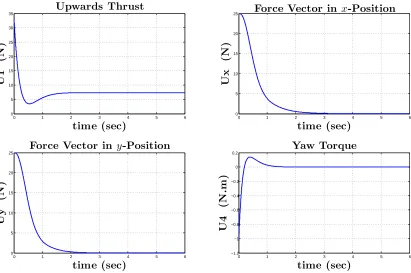
Simulation Results for Backstepping Position Control . . . 56

2.4.6 Spatial Velocity Control for UAV . . . 57

Simulation Results for Backstepping Velocity Control . . . 62

2.5 Conclusion . . . 62

3 Simultaneous Localization and Mapping 66 3.1 Introduction . . . 66

3.2 Structure of Probabilistic SLAM . . . 67

3.2.1 Random Variables and Belief Distributions . . . 67

3.2.2 Map Representations . . . 70

3.2.3 Probabilistic SLAM . . . 72

3.2.4 Parametric Filters . . . 73

3.3 Extended Kalman Filter SLAM Algorithm for a Quadrotor UAV . . . 75

(6)

3.3.2 Observation Model . . . 79

3.3.3 Data Association . . . 81

3.3.4 Constructing EKF-SLAM . . . 83

EKF Prediction Step . . . 84

EKF Update Step . . . 85

System Initialization . . . 85

Adding a new beacon . . . 85

3.4 EKF-SLAM Algorithm . . . 89

4 Teleoperation of UAVs with SLAM-based Haptic Feedback 93 4.1 Introduction . . . 93

4.2 Predictive Displays . . . 94

4.3 SLAM-Based Haptic Feedback . . . 95

4.4 The Artificial Potential Field . . . 97

4.4.1 Models for Artificial Potential Field . . . 99

4.4.2 Experimental results for APFs . . . 102

4.5 Control Structure of a Teleoperator System with SLAM-based Haptic Feedback 110 4.6 Algorithms for SLAM-based haptic feedback . . . 114

4.6.1 Basic SLAM-based haptic feedback algorithm . . . 115

4.6.2 Semi-experimental results for basic SLAM-based haptic feedback al-gorithm . . . 116

4.6.3 Robust SLAM-based haptic feedback algorithm . . . 129

4.6.4 Semi-experimental results for robust SLAM-based haptic feedback al-gorithm . . . 133

(7)

B.1 Introduction . . . 161

B.2 Forward and Inverse Kinematics of Phantom Omni . . . 162

B.3 Jacobian Matrix . . . 163

B.4 OpenHaptics Toolkit . . . 164

Curriculum Vitae 165

(8)

UAV : Unmanned Aerial Vehicle

SLAM: Simultaneous Localization and Mapping EKF: Extended Kalman Filter

APF: Artificial Potential Field

(9)

simultaneously with the same magnitude. The movement direction in this fig-ure is upward. . . 14 2.3 Generating roll torque. Increase in angular velocity of motor 2 and decrease

in angular velocity of motor 4 while keeping the angular velocities of motors 1 and 3 lower than that of motor 2 and greater than that of motor 4 causes the platform to roll aboutxaxis subsequently move in the direction shown. . . 15 2.4 Generating the pitch torque. Increase in angular velocity of motor 3 and

de-crease in angular velocity of motor 1 while keeping the angular velocities of motors 2 and 4 lower than that of motor 3 and greater than that of motor 1 causes the platform to pitch abouty axis subsequently move in the direction shown. . . 16 2.5 Generating yaw torque. Increase in angular velocities of motors 3 and 1 and

decrease in angular velocities of motors 4 and 2 generates clockwise rotation due to drag torque. . . 16 2.6 Two common representations of the inertial frame under the assumption of flat

Earth surface represented by the blue plane, where the golden sphere represents the Earth. . . 17

(10)

2.8 Modeling the rotor as a rotating disk; the figure shows the direction of the air flow through the rotor. . . 19 2.9 General attitude control scheme, whereU1,U2,U3, andU4 are the control

in-puts. . . 22 2.10 General position control scheme, where Ux andUy are the virtual inputs that

control position on thex−yplane. . . 23 2.11 Attitude regulation problem: altitude and attitude errors for PD controller. . . . 25 2.12 Attitude regulation problem: the position (x,y,z) of the center of the

quadro-tor’s mass for PD controller. . . 26 2.13 Attitude regulation problem: magnitude of the control inputs for PD controller. 27 2.14 Attitude regulation problem: altitude and attitude errors for PID controller. . . 29 2.15 Attitude regulation problem: the position (x,y,z) of the center of the

quadro-tor’s mass for PID controller. . . 30 2.16 Attitude regulation problem: the magnitude of the control inputs for the PID

control. . . 31 2.17 Position regulation problem: errors of linear positions and yaw angle for PD

controller. . . 33 2.18 Position regulation problem: the position (x,y,z) of the center of the

quadro-tor’s mass for PD controller. . . 34 2.19 Position regulation problem: the magnitude of the control inputs for PD

con-troller. . . 35 2.20 Attitude regulation problem: altitude and attitude errors for backstepping

con-troller. . . 49 2.21 Attitude regulation problem: the position (x,y,z) of the center of the

quadro-tor’s mass using backstepping controller. . . 50

(11)

2.26 Velocity regulation problem: errors of linear velocies and yaw angle for

back-stepping controller. . . 63

2.27 Velocity regulation problem: the position (x,y,z) of the center of the quadro-tor’s mass for backstepping controller. . . 64

2.28 The magnitude of control inputs of backspteing controller for velocity control (regulation problem). . . 65

3.1 Bell curves of multiple belief distributions. . . 70

3.2 Metric map representations: a feature-based map (left); a cell-based map (right). . . . 71

3.3 Representation of the quadrotor’s frameFL_in_FG _{. . . 76}

3.4 3D sensor that provides observations to a beacon . . . 80

4.1 Simple predictive display model for bilateral teleoperation systems. . . 94

4.2 Structure of the teleoperator system with SLAM-based haptic feedback . . . . 96

4.3 2D illustration of the method for generating the SLAM-based haptic feedback. 97 4.4 Direction of APF force vectors in the vicinity of obstacles. . . 99

4.5 Algorithm 4: APF based on the penetration depth only . . . 100

4.6 Algorithm 5: APF with velocity-dependent term. . . 102

4.7 GUI used in the experiments with 2D APF. . . 104

(12)

force. . . 105

4.9 GUI used in the experiments with 3D APF. . . 107

4.10 Response of 3D APF: the stiffness and the damping components of the reflected force. . . 108

4.11 Control structure of a teleoperator system with SLAM-based haptic feedback. . 110

4.12 An example of a feature-based map of the environment. . . 112

4.13 A virtual environment constructed by EKF-SLAM algorithm on the master side which corresponds to the map in Figure 4.12. . . 113

4.14 3D potential force field around a beacon penetrated by the quadrotor. . . 114

4.15 Illustration of Algorithm 6. . . 116

4.16 The trajectory of the quadrotor on the slave side. . . 117

4.17 Estimates of the beacons’ locations at the master side (blue spheres) vs. true locations (shaded red spheres). . . 118

4.18 Basic SLAM-based haptic feedback: GUI which shows the master (left) and slave (right) sides. . . 119

4.19 Basic SLAM-based haptic feedback experiment, beacon 1. Estimated and true location vs. time (left); estimation errors vs. time (right). . . 121

4.20 Basic SLAM-based haptic feedback experiment, beacon 1. Magnitude of the reflected force vs. time (left); APF penetration distance vs. time (right). . . 122

4.21 Basic SLAM-based haptic feedback experiment, beacon 1. The reflected force components along x, y, and z axes vs. time. . . 122

4.22 Basic SLAM-based haptic feedback experiment, beacon 2. Estimated and true location vs. time (left); estimation errors vs. time (right). . . 123

4.23 Basic SLAM-based haptic feedback experiment, beacon 2. Magnitude of the reflected force vs. time (left); APF penetration distance vs. time (right). . . 124

(13)

components along x, y, and z axes vs. time. . . 126 4.28 Basic SLAM-based haptic feedback experiment, beacon 4. Estimated and true

location vs. time (left); estimation errors vs. time (right). . . 127 4.29 Basic SLAM-based haptic feedback experiment, beacon 4. Magnitude of the

reflected force vs. time (left); APF penetration distance vs. time (right). . . 128 4.30 Basic SLAM-based haptic feedback experiment, beacon 4. The reflected force

components along x, y, and z axes vs. time. . . 128 4.31 3D Gaussian distribution represented as an ellipsoid with different confidence

levels. . . 130 4.32 The side-effect of buidling a fixed APF where the green, red, yellow, blue

shapes represent APF, a possible true location of a beacon, a beacon’s estimate and the ellipsoid of the beacon’s estimate. . . 131 4.33 Uncertainty-dependent artificial potential field (UDAPF). . . 132 4.34 Robust SLAM-based haptic feedback experiment, beacon 1. Estimated and

true location vs. time (left); estimation errors vs. time (right). . . 135 4.35 Robust SLAM-based haptic feedback experiment, beacon 1. Magnitude of the

reflected force vs. time (left); APF penetration distance vs. time (right). . . 136 4.36 Robust SLAM-based haptic feedback experiment, beacon 1. The reflected

force components along x, y, and z axes vs. time. . . 136

(14)

true location vs. time (left); estimation errors vs. time (right). . . 137

4.38 Robust SLAM-based haptic feedback experiment, beacon 2. Magnitude of the reflected force vs. time (left); APF penetration distance vs. time (right). . . 138

4.39 Robust SLAM-based haptic feedback experiment, beacon 2. The reflected force components along x, y, and z axes vs. time. . . 138

4.40 Robust SLAM-based haptic feedback experiment, beacon 3. Estimated and true location vs. time (left); estimation errors vs. time (right). . . 139

4.43 Robust SLAM-based haptic feedback experiment, beacon 4. Estimated and true location vs. time (left); estimation errors vs. time (right). . . 141

A.1 Venn diagram for the dependency and independency of two events. . . 159

A.2 Venn diagram that illustrates the total probability theorem. . . 160

B.1 Phantom Omni . . . 161

B.2 Forward and Inverse Kinematics [3] . . . 162

B.3 OpenHaptics Toolkit [2]. . . 164

(15)

2.6 Backstepping controller parameters for linear velocity control (regulation task) 62

4.1 The numerical parameters of stiffness and damping terms for 2D APF. . . 103 4.2 The numerical parameters of stiffness and damping terms for 3D APF. . . 104 4.3 Basic SLAM-based haptic feedback: True locations of Beacons at the Slave side.118 4.4 The workspace of the Phantom Omni. . . 119 4.5 Locations of beacons at the slave side . . . 133 4.6 Backstepping controller parameters for robust SLAM-based haptic feedback

algorithm. . . 134

(16)

Appendix A:Basic Probability Notions Appendix B:Phantom Omni Device

(17)

three major areas of engineering to which this thesis is related, which are Unmanned Aerial Vehicles (Section 1.1), Simultaneous Localization and Mapping (Section 1.2), and Haptics and Teleoperation (Sections 1.3-1.5). Motivation behind the research presented in this thesis is discussed in Section 1.6. Thesis contribution is described in Section 1.7, and thesis outline is given in Section 1.8.

1.1 Unmanned Aerial Vehicles

Recent advances in a number of engineering disciplines have lead to development and fabri-cation of efficient and powerful Unmanned Aerial Vehicles (UAVs). An UAV is defined as a machine that is capable of flying remotely without the presence of a human operator in the control cabin [4]. The ability of UAVs to perform tasks without the presence of a human oper-ator inside the vehicle makes them suitable for numerous applications, particularly those where safety of the pilot is a major concern. Popularity of UAVs has recently increased drastically due to their applications to both military and civilian tasks [5, 6, 7, 8]. In the past, the usage of UAVs was mostly limited to military missions, however, currently there also exists substantial

(18)

and growing demand for UAVs in civilian applications [9]. In particular, UAVs can be used for scientific research [9], agricultural tasks [10], surveillance [11], mine scanning [12], search and rescue [13], aerial photography [14],etc. One of the most fascinating and promising civil-ian applications was recently announced in a letter submitted by Amazon company to the U.S. Federal Aviation Administration on July 9, 2014, which states that delivery of customers’ or-ders might be done in 30 minutes or less by using UAVs [15]. For a survey of some current and potential applications of UAVs, both military and civilian, the reader is referred to [9].

A class of UAVs that are capable of take-off and landing vertically is known as VTOL (Vertical Take-Off and Landing) UAVs [16]. This class of aerial vehicles does not require runways, which makes them a natural choice for missions that require quick and flexible access to the incident place, such as search and rescue missions. Another important advantage of VTOL over fixed-wing aircrafts is their manoeuvrability which, in particular, allows for flying in confined spaces and/or over difficult terrains. Nowadays, VTOL vehicles come in a variety of sizes such as heavy, normal, small, mini-small, and even micro, and may have different structures such as a single rotor, two side by side rotors, two rotors with coaxial configuration, and multi-rotors [4]. The most common multi-rotor configuration is the quadrotor (four rotors aircraft), which is the type of UAV addressed in this thesis.

1.2 Simultaneous Localization and Mapping

(19)

proaches are not suitable for fully autonomous navigation, and that uncertainty must be taken into account. Nowadays, the dominant approaches for solving SLAM problem are based on probabilistic methods. From probabilistic perspective, SLAM problem can be formulated as follows: given noisy measurements and control inputs, find the probability distribution of the current state of robot and the environment under the assumption that the environment isa priori

unknown. In Chapter 3, it will be shown how can such a probability distribution be computed using recursive Bayesian approach.

(20)

SLAM. The obtained results show the reliability of the visual SLAM for estimating the posi-tion of the platform relative to observed landmarks in outdoor environments. Paper [23] is an example of applications of SLAM to indoor environments. In this work, SLAM is implemented on a semi-autonomous UAV equipped with 3D laser sensor which is capable of navigating in demolished buildings and designed for handling radioactive materials. For some survey related to applications of SLAM, the reader is referred to [24, 25].

1.3 Haptic Technology

The word “haptics” is derived from a Greek word “ ´απτω” which means “touch” [26]. Haptic technology deals with exchanging information between the machine and a human being via the sense of touch. Nowadays, multimedia is not restricted to visual and audio feedback; in particular, haptic technology can be used in virtual environments to create more realistic scenarios. Haptic feedback become essential in numerous applications such as pilots training, surgical training, computer-aided design, and entertainment.

(21)

Figure 1.1: Scientific and engineering disciplines related to haptics [1].

1.4 Teleoperation

(22)

Human

Operator Master

Communication

Channel Slave

Remote Environment

Figure 1.2: Teleoperation system structure.

The structure of a typical single-master-single-slave bilateral teleoperator system is shown in Figure 1.2. It consists of five components, which are the human operator, the master de-vice, the slave dede-vice, an environment, and a communication channel between the master and the slave [34, 35]. The human operator controls the master device, which communicates its position, velocity, and sometimes acceleration to the remotely located slave. The slave robot follows the motion of the master thus executing a task on the remote environment. On the other hand, the slave device typically has an ability to sense the forces exerted on it due to the inter-action with the remote environment; information about these forces is transferred back to the master over the communication channel. These interaction forces are subsequently presented to the human operator in the form of haptic feedback. The haptic feedback allows the human operator to feel the remote interaction, which leads to improved situation awareness and higher performance of teleoperation. Transparencyis a measure of how well the teleoperator system replicates the motion/forces on the opposite side. A perfectly transparent teleoperator system creates an illusion for the human operator as if the task is executed directly.

1.5 Visual and Haptic Feedback in Teleoperation

(23)

clues. In UAVs teleoperation, this implies that the human operator may not be able to perceive whether the platform is getting closer to or going away from the obstacles.

Providing more than one camera to acquire depth perception (such as stereo vision) is a classical solution, however, it may be unsuitable in some cases due to the fact that the payload of the platform and complexity of manipulating images will increase drastically. Moreover, cameras provide information only in the direction of view and the visual information may be limited due to occlusions; this is commonly known as the limited field of view problem. In particular, the human operator may not be able monitor blind spots to avoid potential collision. Another common modality that is known to enhance the human operator’s awareness in teleoperation is haptic feedback. Haptic feedback has some advantages over its visual counter-part. For example, the environment surrounding the slave device can be mapped into artificial force field, which eliminates the limited field of view problem. The human operator reacts faster to haptic feedback than to visual feedback [36]. Moreover, the receptors of haptic feed-back covers the whole body of the human operator which means it is not limited to specific organs like ears for audition and eyes for vision [37, 38]. Another unique characteristic of hap-tic feedback is that the energy flow between the sender and the receiver is bidirectional [39]; in other words, action and perception are not separated in the case of haptic feedback.

(24)

that, in the presence of time delay, the communication channel is no longer a passive subsys-tem [34]. There are numerous approaches reported in the literature that deal with instability of teleoperation systems that occurs due to delayed haptic feedback. For example,wave variables approach stabilizes a force-reflecting bilateral teleoperator by encoding force and velocity vari-ables into another set of varivari-ables known as wave varivari-ables, see [43, 33]. The wave varivari-ables are then sent via the communication channel and decoded once they are received to extract the force and velocity. This approach guarantees stability if the time delay is constant [44]. Other approaches suggest to abandon haptic feedback altogether and utilize other modalities such visual, auditory, vibrotactile, and graphical feedbacks to display forces. This approach is known as sensory substitution[45, 46, 47, 48]. One more approach to deal with instability of bilateral teleoperation generated by time delays is to rely on a virtual model of the remote environment at the master side to acquire the haptic feedback rather than exchanging haptic data over the communication channel. This approach is based on usingpredictive displays, and is described in Section 4.2.

1.6 Motivation

(25)

build-spaces for which a detailed map is not available. Therefore, there is a need for development of a teleoperator system with the ability to build a virtual model of the remote environment in real-time while executing the task on the actual remote environment.

1.7 Thesis Contribution

(26)

The SLAM techniques, on the other hand, are currently directed to applications where the pri-mary goal is to make the robot as autonomous and independent of the human intervention as possible. This thesis is apparently the first work where the SLAM and the haptic technologies are combined together to solve a meaningful technological problem.

1.8 Thesis Outline

The structure of the remaining part of the thesis can be described as follows:

In Chapter 2, the kinematics, dynamics, and control algorithms for a quadrotor UAV are ad-dressed. In particular, both attitude control and position control problems are formulated, and the control strategies for both linearized and fully nonlinear models of the quadrotor are developed in detail. In the case of linearized model, PD and PID controllers are used, while the control strategies for nonlinear model are based on the integrator backstepping approach. Comprehensive mathematical derivation of the backstepping control algo-rithm for a quadrotor UAV is provided. In both cases of linearized and nonlinear models, simulations have been carried out using Matlab and C++to evaluate the performance of the controllers, and the results are discussed.

In Chapter 3, the problem of Simultaneous Localization and Mapping (SLAM) is addressed from probabilistic perspective. A general form of probabilistic SLAM approach based on Bayesian framework is presented. Different types of metric maps and parametric filters are discussed. The Extended Kalman Filter (EKF) implementation of the SLAM algorithms is described in detail, and a complete EKF-SLAM algorithm for a quadrotor UAV is developed.

(27)

the covariance estimate provided by EKF. Semi-experimental results are presented that evaluate performance of the developed teleoperator system with SLAM based haptic feedback.

(28)

Kinematics, Dynamics, and Control of a

Quadrotor UAV

In this Chapter, kinematics, dynamics, and control of a quadrotor aircraft are addressed. Sec-tion 2.1 gives a general introducSec-tion into quadrotor operaSec-tion and shows how forces/torques generated by the rotors affect the platform’s movement. Section 2.2 discusses the basics of quadrotor’s kinematics. Section 2.3 focuses on the dynamic behaviour of the quadrotor; in particular, it shows how the dynamic equations can be derived using Euler-Newton approach. Section 2.4 deals with control algorithms for quadrotor. In this section, linear and nonlinear models of the quadrotor are addressed, and algorithms for attitude control and position control are derived, with special emphasis on the nonlinear control design using backstepping meth-ods. Numerical simulations of different control algorithms are performed using Matlab and C++, and the results are presented. Conclusions are given in Section 2.5.

2.1 Basic Quadrotor Operation

The quadrotor platform is an example of VTOL UAVs with cross configuration that has four propellers connected separately to four motors which play the role of actuators. The configu-ration space of a quadrotor has 6 degrees-of-freedom (DOFs), which include three DOFs for

(29)

Fi =kFω2i, (2.1)

Mi =kMω2i, (2.2)

where kF and kM are constants that can be acquired through an experimental test [49], [50]. Figure 2.1 shows a top view of the platform, where the red arrows denote the rotational

direc-ω2

Motor 2

Motor 4

ω4

ω1

Motor 1

Motor 3

ω3

Figure 2.1: Cross configruation of the quadrotor, view from the top.

tion of propellers; specifically, Motors 1 and 3 rotate counter-clockwise whereas Motors 2 and 4 rotate clockwise. NotationUis the control input which can be force or torque. Theupwards thrust U1is defined as follows,

U1 = 4 X

i=1

(30)

NotationU1 in (2.3) represents the total force that is responsible for lifting the quadrotor up.

The pure upwards thrust is generated when all motors are rotated with the same angular ve-locity, see Figure 2.2. In the aforementioned figure, the axes of the body frame are defined in which the positive part of thezaxis points to the ground. Theroll torque U2 is the torque

x y

z ω2

Motor 2

Motor 4 ω4 ω1 Motor 1

Motor 3 ω3

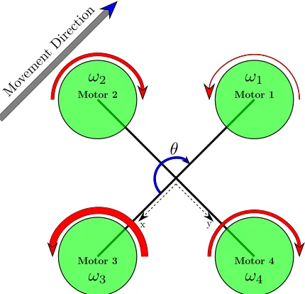
Movement Direction

Figure 2.2: Generating the upwards thrust by increasing/decreasing all motors’ velocities si-multaneously with the same magnitude. The movement direction in this figure is upward.

that causes the platform to rotate about its x-axis. It is generated by increasing the angular velocity of motor 2 and decreasing the angular velocity of motor 4 for achieving the clockwise rotation (i.e., the right turn), see Figure 2.3. For the counter-clockwise rotation about x-axis, the process is reversed,i.e., the angular velocity of motor 4 increases and the angular velocity of motor 2 decreases. The formula for roll torqueU2is as follows:

U2 =l(F4−F2), (2.4)

wherelis the distance from each rotor to the center of the quadrotor’s mass. Thepitch torque U3is the torque that causes the platform to rotate about itsy-axis. It is generated by increasing

(31)

x y

Motor 4

ω4

Motor 3

ω3

Figure 2.3: Generating roll torque. Increase in angular velocity of motor 2 and decrease in angular velocity of motor 4 while keeping the angular velocities of motors 1 and 3 lower than that of motor 2 and greater than that of motor 4 causes the platform to roll about xaxis subsequently move in the direction shown.

is given as follows,

U3 =l(F3−F1). (2.5)

Theyaw torque U4 is the torque that causes the platform to rotate about itsz-axis. Whenever

the angular velocities of motors 3 and 1 increase with same magnitude while the angular ve-locities of the other two motors decrease, a drag torque is generated that causes the platform to rotate in the direction opposite to the rotations of motors 3 and 1. Figure 2.5 shows the rotation of the platform in the clockwise direction.

U4 =Kw(F3+F1−F4−F2), (2.6)

(32)

x y

ω2

Motor 2

Motor 4

ω4 ω1

Motor 1

Motor 3

ω3

θ

Movem

ent Direction

Figure 2.4: Generating the pitch torque. Increase in angular velocity of motor 3 and decrease in angular velocity of motor 1 while keeping the angular velocities of motors 2 and 4 lower than that of motor 3 and greater than that of motor 1 causes the platform to pitch aboutyaxis subsequently move in the direction shown.

x y

ω2 Motor 2

Motor 4

ω4

ω1 Motor 1

Motor 3

ω3

ψ

z

Movement Direction

(33)

respectively. The center of an inertial frame FI _{is usually attached to a given point on the} Earth’s surface; the latter is assumed to be flat [53]. One possible configuration of the inertial frame is such that its x-, y-, and z-axes are directed towards the North, East, and the center of the Earth, respectively. This type of frame configuration is known as North-East-Down (NED) coordinate system [54]. Another possible configuration of the inertial frame is where the x-, y-, and z-axes point toward the East, North, and in the Upward direction (ENU), respectively [55]. Figure 2.6 shows the NED and the ENU coordinate systems. On the other hand, thebody

(a) North-East-Down (NED) coordinate system (b) East-North-Up (ENU) coordinate system

Figure 2.6: Two common representations of the inertial frame under the assumption of flat Earth surface represented by the blue plane, where the golden sphere represents the Earth.

(34)

posi-xI O_FI

yI

zI

xB O_FB

yB

zB

(a) Body frame in (NED)

xI O_FI

yI

zI

xB O_FB

yB

zB

(b) Body frame in (ENU)

Figure 2.7: The representations of the body frame in NED and ENU coordinates.

tion of the center of quadrotor’s mass is specified in the inertial frame through three variables denoted as x,yand z, whereas the orientation of the quadrotor in the body frame is specified through three anglesφ, θ andψ, that describe the rotation around xB_, _yB_{, and}_zB _axes, respec-tively. Orientation of a rigid body in 3D space can be carried out using various methods. The most common and widely used approach is based onEuler angles[56, 54, 57]. This method describes orientation of a rigid body in 3D space by specifying three angles known asyaw(ψ), pitch(θ) androll(φ).

2.3 Quadrotor Dynamics

The dynamics of a rigid body describe the relationship between the motion of the body in space and the forces/torques that cause this motion. In the case of the quadrotor system, the primary forces (i.e.,F1,F2,F3, andF4) that cause the quadrotor to fly are generated by the four motors.

Thei-th spinning rotor contributes to the whole upwards thrust by generating the vertical thrust

Fiand the drag torque Mi, which are given by the following formulas [58]:

Fi =CFρAω2iR

2_,

(2.7)

Mi =CMρAω2iR

(35)

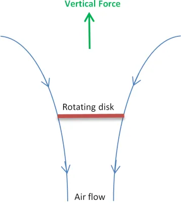
between the upwards thrust that a propeller generates, the induced velocity, and the induced power of the rotor via Bernoulli’s equation [59]. The dynamics of the quadrotor are also

sub-Figure 2.8: Modeling the rotor as a rotating disk; the figure shows the direction of the air flow through the rotor.

ject to external forces that impede quadrotor’s motion. For the sake of simplicity, it is assumed throughout this thesis that the only external force that acts on the quadrotor’s body is the gravi-tational forceFg. The dynamics of the quadrotor are a combination of the translational and the rotational dynamics [7], in which the translational dynamics depend on the rotational dynamics but notvice versa, as will be shown below.

(36)

applies Newton’s laws directly to derive the mathematical model of the quadrotor by consid-ering all forces/torques that cause the motion. The general form of the dynamics equations of an aerial vehicle under the influence of external forces/torques can be expressed through the following equations:

˙

Υ =V, (2.9)

mV˙ = F_Υ, (2.10)

˙

R= RΩˆ, (2.11)

Ω =˙ −Ω×Ω +Mη, (2.12)

whereΥ := (x,y,z) ∈ R3 _{is the position of the center of quadrotor’s mass and} _V _∈ _R3 _{is the}

linear velocity of the center of the quadrotor’s mass expressed in the inertial frame,F_Υ ∈R3and

Mη∈R3are the vectors of translational forces and rotational moments, respectively,Ω∈R3is

the angular velocity expressed in the body frame, ˆΩ ∈R3×3 _{is a skew symmetric matrix which}

is defined as follows,

ˆ Ω =                    

0 −Ω₃ Ω₂

Ω3 0 −Ω1

−Ω₂ Ω₁ 0

                   

andR∈S O(3) is the orthogonal rotation matrix.

The mathematical model of the quadrotor in this thesis is adopted from [55]; according to this work, the dynamics of the quadrotor are described by the following nonlinear equations:

¨

x= U1

m(cosφsinθcosψ+sinφsinψ), (2.13)

¨

y= U1

m(cosφsinθsinψ−sinφsinψ), (2.14)

¨

z= U1

m(cosφcosθ)−g, (2.15)

¨

φ= Jy−Jz

Jx

˙

θ_ψ˙ ₊ l

Jx

U2, (2.16)

¨

θ = Jz−Jx

Jy

˙

φ_ψ˙ ₊ l

Jy

(37)

Jx Inertia moment about x-axis 0.019688 kgm2

Jy Inertia moment abouty-axis 0.019681 kgm2

Jz Inertia moment aboutz-axis 0.03938 kgm2

2.4 Quadrotor Control Strategy

(38)

Controller

d



d

 d

 d

z

Qaudrotor (t)

) (t

 ) (t z

) (t z

) (t x

) (t x

) (t y

) (t y

) (t



) (t

 ) (t



) (t



1 U

2 U

3 U

4 U

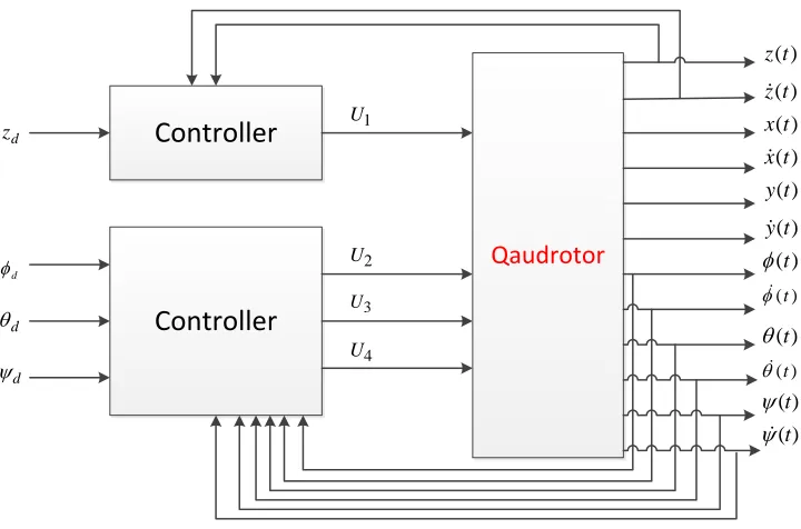
Figure 2.9: General attitude control scheme, whereU1,U2,U3, andU4are the control inputs.

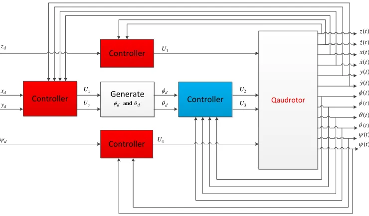
manner. Position control is more difficult than the attitude control due to the fact that the system is underactuated. In literature, the common approach for position control is implementing two control loops called outer and inner loops instead of just one control loop as in the attitude control case. Figure 2.10 shows a general block diagram for position control, in whichxd and

yd represent the desired position in x−yplane, respectively. The red blocks define the outer loop whereas the blue one defines the inner loop. The popular controllers for stabilizing the linearized model of the platform include PD, LQR, PID controllers, among others.

2.4.1 Control Strategy for Linear Model

Using small angle assumption (i.e., assuming the quadrotor is approximately in the hovering state), the following approximations [60] can be used to linearize the platform’s model,

(39)

d

 (t)

) (t  Controller U4

Figure 2.10: General position control scheme, where Ux and Uy are the virtual inputs that control position on thex−yplane.

cos$≈ 1, sin$≈$.

Consequently, the nonlinear model (2.13)-(2.18) can be reduced to the following linearized model,

¨

x= gθ, (2.19)

¨

y= −gφ, (2.20)

¨

z= U1

m −g, (2.21)

¨

φ= L

Jx

U2, (2.22)

¨

θ= L

Jy

U3, (2.23)

¨

ψ= 1

Jz

(40)

Attitude Control for Linear Model

In theattitude regulationproblem, the desired rollφd, pitchθd, and yawψd angles, as well as the desired altitudezdare assumed constant, and the goal is to achieve asymptotic convergence of the actual variables φ, θ, ψ and z to their desired constant values, and the convergence of the corresponding velocities to zero. Mathematically, the goal is to guarantee thatφ(t) → φd,

θ(t) → θd,ψ(t)→ ψd,z(t) → z, and ˙φ(t) → 0, ˙θ(t)→ 0, ˙ψ(t) → 0, ˙z(t) → 0 ast → ∞. Using PD controller, the control inputs for the attitude control can be specified as follows

U1 =m g+Kzp(zd −z)+K_dz

d

dt(zd−z)

!

, (2.25)

U2 = Kφp(φd−φ)+K φ d

d

dt(φd−φ), (2.26)

U3 = Kθp(θd−θ)+Kdθ

d

dt(θd−θ), (2.27)

U4 = Kψp(ψd−ψ)+K ψ d

d

dt(ψd−ψ), (2.28)

where Kp% > 0 and K %

d > 0 are the proportional and derivative gains, respectively, and % ∈

{z, φ, θ, ψ}. In order to illustrate the performance of the PD controller in the attitude regulation problem, the closed-loop system (2.19)-(2.28) was simulated in Matlab. Table 2.1 presents numerical values of the parameters used in the simulations, while Figures 2.11, 2.12, and 2.13 show the response of the quadrotor.

initial values Gains Desired Trajectory

Altitude z(0)=0 ˙

z(0)=0

Kzp =12.34

K_dz = 5.67

zd = 5 (m) Roll φ(0)= π₄

˙

φ(0)=0

Kφp =11.2

K_dφ =4.2

φd =0 (rad) Pitch θ(0)= π₄

˙

θ(0)=0

Kθ_p =9.7

K_dθ =3.6

θd =0 (rad) Yaw ψ(0)= π₃

˙

ψ(0)=0

Kψp = 10.78

K_dψ = 5.2

ψd = 0 (rad)

(41)

0 0.5 1 1.5 2 2.5 3 3.5 4 4.5 5 −5 −4 −3 −2 −1 0

1 Altitude Error

time (sec) zd − z ( t ) (m )

0 0.5 1 1.5 2 2.5 3 3.5 4 4.5 5 −0.1 0 0.1 0.2 0.3 0.4 0.5 0.6 0.7

0.8 Roll Error

time (sec) φd − φ ( t ) (r a d )

0 0.5 1 1.5 2 2.5 3 3.5 4 4.5 5 −0.1 0 0.1 0.2 0.3 0.4 0.5 0.6 0.7

0.8 Pitch Error

time (sec) θd − θ ( t ) (r a d )

0 0.5 1 1.5 2 2.5 3 3.5 4 4.5 5 −0.2 0 0.2 0.4 0.6 0.8 1

1.2 Yaw Error

time (sec) ψd − ψ ( t ) (r a d )

(42)

0 2

4 6

8 10

12 14

16 18

−15 −10

−5 0

0 1 2 3 4 5 6

x _(m)

Quadrotor Position (x, y, z₎

y _(m)

z

(m

)

(43)

0 0.5 1 1.5 2 2.5 3 3.5 4 4.5 5 −0.6 −0.5 −0.4 −0.3 −0.2 −0.1 0 0.1 0.2 Pitch Torque time (sec) U 3 (N .m )

0 0.5 1 1.5 2 2.5 3 3.5 4 4.5 5 −0.5 −0.4 −0.3 −0.2 −0.1 0 0.1 0.2 Yaw Torque time (sec) U 4 (N .m )

Figure 2.13: Attitude regulation problem: magnitude of the control inputs for PD controller.

In PID controller, a new term (i.e., the integral term) is added to the PD controller, therefore the control inputs can be specified as follows

U1= m· g+Kzp(zd−z)+K_dz

d

dt(zd−z)+K

z i

Z t

0

(zd−z(τ))dτ

!

, (2.29)

U2= Kφp(φd−φ)+K φ d

d

dt(φd−φ)+K

φ i

Z t

0

(φd−φ(τ))dτ, (2.30) U3= Kθp(θd−θ)+Kdθ

d

dt(θd−θ)+K

θ i

Z t

0

(θd−θ(τ))dτ, (2.31) U4= Kψp(ψd−ψ)+K_dψ

d

dt(ψd−ψ)+K

ψ i

Z t

0

(44)

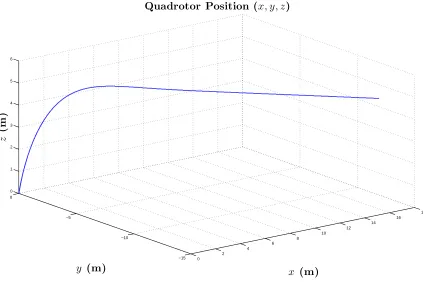
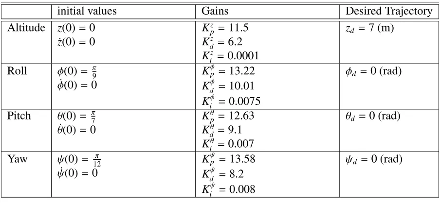
initial values Gains Desired Trajectory Altitude z(0)=0

˙

z(0)=0

Kz

p =11.5

K_dz = 6.2

K_iz =0.0001

zd = 7 (m)

Roll φ(0)= π₉ ˙

φ(0)=0

Kφp =13.22

K_dφ =10.01

K_iφ =0.0075

φd =0 (rad)

Pitch θ(0)= π₇ ˙

θ(0)=0

Kθ_p =12.63

K_dθ =9.1

K_iθ =0.007

θd =0 (rad)

Yaw ψ(0)= ₁₂π ˙

ψ(0)=0

Kψp = 13.58

K_dψ = 8.2

K_iψ = 0.008

ψd = 0 (rad)

Table 2.2: PID controller parameters for the attitude regulation problem

Position Control for the Linear Model

It can be noticed from equations (2.19)-(2.20) that the linear accelerations ¨x and ¨y can not be controlled directly. However, the aforementioned linear accelerations depend on the roll and pitch angles. One can exploit this fact to control xandyindirectly through appropriately designed desired (reference) trajectories for rollφd(t) and pitchθd(t) angles [50]. Specifically, let the desired pitch and roll angles be defined as follows,

θd := Ux

g , (2.33)

φd := − Uy

g , (2.34)

whereUxandUyare virtual control inputs forxandylinear positions, respectively. Assuming

θ=θd,φ= φd, one sees from (2.19), (2.20) that

¨

x= Ux,

¨

(45)

0 1 2 3 4 5 6 7 8 9 −7 −6 −5 −4 −3 −2 −1 0

1 Altitude Error

0 1 2 3 4 5 6 7 8 9

−0.1 −0.05 0 0.05 0.1 0.15 0.2 0.25 0.3

0.35 Roll Error

0 1 2 3 4 5 6 7 8 9

−0.1 0 0.1 0.2 0.3 0.4 0.5

0.6 Pitch Error

0 1 2 3 4 5 6 7 8 9

−0.1 −0.05 0 0.05 0.1 0.15 0.2 0.25

0.3 Yaw Error

(46)

0 1

2 3

4 5

6 7

−5 −4.5 −4 −3.5 −3 −2.5 −2 −1.5 −1 −0.5 0 0 1 2 3 4 5 6 7 8

x _(m)

Quadrotor Position (x, y, z₎

y _(m)

z

(m

)

(47)

0 1 2 3 4 5 6 7 8 9 −10

0 10 20 30 40 50 60

70 Upwards Thrust

time (sec)

U

1

(N

)

0 1 2 3 4 5 6 7 8 9

−0.4 −0.35 −0.3 −0.25 −0.2 −0.15 −0.1 −0.05 0

0.05 Roll Torque

time (sec)

U

2

(N

.m

)

0 1 2 3 4 5 6 7 8 9

−0.45 −0.4 −0.35 −0.3 −0.25 −0.2 −0.15 −0.1 −0.05 0 0.05

Pitch Torque

time (sec)

U

3

(N

.m

)

0 1 2 3 4 5 6 7 8 9

−0.16 −0.14 −0.12 −0.1 −0.08 −0.06 −0.04 −0.02 0

0.02 Yaw Torque

time (sec)

U

4

(N

.m

)

(48)

The virtual control inputsUxandUycan now be defined as follows,

Ux = Kpx(xd−x)+K_dx

d

dt(xd−x), (2.35)

Uy = Kyp(yd−y)+K y d

d

dt(yd−y). (2.36)

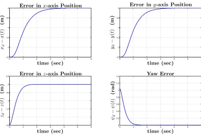
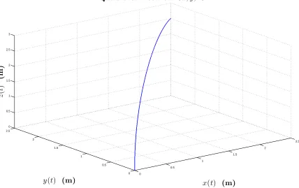
In Matlab, simulations have been carried out to illustrate the performance of the PD controller. Table 2.3 shows the numerical values of the parameters for the simulations and Figures 2.17, 2.18, and 2.19 show the response of the quadrotor.

initial values Gains Desired Value

Altitude z(0)=0 ˙

z(0)=0

Kz

p =14

Kz_d =7

zd = 2.5 (m) x-Position x(0)=0

˙

x(0)=0

Kx

p = 10

K_dx = 5

xd = 2.5 (m) y-Position y(0)=0

˙

y(0)=0

Kyp =10

Ky_d =5

yd = 2.5 (m) Yaw ψ(0)= π₃

˙

ψ(0)=0

Kψp =25

Kψ_d =10

ψd = 0 (rad)

Roll φ(0)=0

˙

φ(0)=0

Kφp =21.3

Kφ_d =12.72

Pitch θ(0)=0 ˙

θ(0)=0

Kθ_p =19.5

Kθ_d =9.7

Table 2.3: PD controller parameters for position regulation problem

2.4.2 Control Strategy for Nonlinear Quadrotor Model

(49)

0 1 2 3 4 5 6 −2.5 −2 −1.5 −1 −0.5

0 Error in

x_{-axis Position}

time (sec) xd − x ( t ) (m )

0 1 2 3 4 5 6

−2.5 −2 −1.5 −1 −0.5

0 Error in

y_{-axis Position}

time (sec) yd − y ( t ) (m )

0 1 2 3 4 5 6

−2.5 −2 −1.5 −1 −0.5 0

0.5 Error in

z_{-axis Position}

0 1 2 3 4 5 6

0 0.2 0.4 0.6 0.8 1 1.2

1.4 Yaw Error

(50)

0

0.5

1

1.5

2

2.5

0 0.5 1

1.5 2

2.5 0 0.5 1 1.5 2 2.5 3

x₍t₎ _(m)

Quadrotor Position < x, y, z >

y₍t₎ _(m)

z

(

t

)

(m

)

(51)

0 1 2 3 4 5 6 0

5 10 15 20 25 30

35 Upwards Thrust

time (sec)

U

1

(N

)

0 1 2 3 4 5 6

0 5 10 15 20

25 Force Vector in

x_-Position

time (sec)

U

x

(N

)

0 1 2 3 4 5 6

0 5 10 15 20

25 Force Vector in

y_-Position

time (sec)

U

y

(N

)

0 1 2 3 4 5 6

−1.2 −1 −0.8 −0.6 −0.4 −0.2 0

0.2 Yaw Torque

time (sec)

U

4

(N

.m

)

(52)

predetermined surface in the state space called the sliding surface [64, 65]. In [66, 61, 67, 55], the sliding mode controller has been used for quadrotor control. Feedback linearization con-trollers are another class of concon-trollers that target nonlinear systems by cancelling all sub-stantial nonlinearties; as a result, the closed-loop system becomes linear and therefore can be controlled using linear methods. In [68, 69], the feedback linearization approach has been used to stabilize the quadrotor. In this thesis, we concentrate on the Lyapunov-based backstepping control method, therefore the following sections deal with control algorithms that are based on the backstepping approach.

2.4.3 Backstepping Controller

In [70], which is currently the most comprehensive book that deals with backstepping control methods, the backstepping is defined as an approach ”to design a controller recursively by considering some of the state variables as ”virtual controls” and designing for them

inter-mediate control laws”[70]. The word “backstepping” comes from the fact that it is essentially

(53)

1

a1:= zd(t)−z(t), (2.37)

where zd(t) and z(t) are the desired and the actual altitudes, respectively. From now on, the independent time variable will be omitted for simplicity of notation. Let a Lyapunov function

V(a1) be defined to be a positive definite function ofa1, as follows,

V(a1)=

1 2a

2

1. (2.38)

Taking into account (2.37), the time derivative of Lyapunov function (2.38) is

˙

V(a1)=a1(˙zd−z˙). (2.39) To make the expression (2.39) bounded from above by some negative definite function, we would like to guarantee that ˙V(a1) satisfies the following inequality,

˙

V(a1)≤ −κ1a21, (2.40)

whereκ1 >0 is a constant. Using (2.39), inequality (2.40) becomes

a1(˙zd−z˙)≤ −κ1a21. (2.41)

Inequality (2.41) is guaranteed if the state variable ˙zsatisfies

˙

z= ˙zd+κ1a1. (2.42)

(54)

used as a virtual control for the purpose of stabilization. To this end, define

zvir :=z˙d+κ1a1. (2.43)

The above defined variablezvirrepresents the desired value of the state variable ˙z,i.e., the value of ˙zthat would guarantee the exponential convergencea1(t)→0.

Step two. Let a new variable a2 be defined as the difference between the state variable ˙z

and the virtual control inputzvir, as follows,

a2 :=z˙−zvir. (2.44)

Using (2.44), the expression (2.39) for ˙V(a1) can be rewritten to yield the following formula

˙

V(a1)=a1(˙zd−z˙)=a1(˙zd−(a2+zvir))

=a1(˙zd−(a2+z˙d+κ1a1))=a₁z˙_d −a₁a₂−

a1z˙d −κ1a21

=−a1a2−κ1a21. (2.45)

Let us now augment the Lyapunov function (2.38) with an additional termV(a2) := 1₂a2₂which

accounts for the dynamics of variablea2. The total Lyapunov functionV(a1,a2) has a form

V(a1,a2) :=V(a1)+V(a2)=

1 2a

2

1+

1 2a

2 2

= 1

2(zd−z)

2₊ 1

2(˙z−zvir)

2₌ 1

2(z

2

d−2zzd+z2)+ 1 2(˙z

2₋

2˙zzvir+z2vir) = 1

2(z

2

d−2zzd+z2)+ 1 2z˙

2₋_z_˙_(˙_z

d+κ1zd−κ1z)

+ 1 2(˙z

2

d+2κ1z˙dzd−2κ1z˙+κ21z 2

d−2κ

2

1zdz+κ2₁z2)

(2.46)

The time derivative of the total Lyapunov functionV(a1,a2) is given by the following

expres-sion

˙

(55)

The exponential convergencea1(t) anda2(t) to zero will be guaranteed if the time derivative of

the total Lyapunov functionV(a1,a2) satisfies the inequality

˙

V(a1,a2)≤ −κ1a21−κ2a22, (2.49)

whereκ1, κ2 >0. Taking into account (2.48), inequality (2.49) becomes

a2z¨−a2(¨zd−κ1(a2+κ1a1))−a1a2

−κ₁a2₁ ≤

−κ₁a2₁ −κ₂a2₂,

or

a2z¨−a2(¨zd−κ1(a2+κ1a1))−a1a2 ≤ −κ2a22. (2.50)

The last inequality (2.50) is satisfied if the following relation holds

¨

z= a1+(¨zd−κ1(a2+κ1a1))−κ2a2. (2.51)

Indeed, substituting (2.51) into (2.50), one obtains

a2[a1+(¨zd−κ1(a2+κ1a1))−κ2a2)−a2(¨zd−κ1(a2+κ1a1))−a1a2

=(a₂a₁ +

((((

(((

a2(¨zd−κ1(a2+κ1a1))−a2κ2a2)−

((((

(((

a2(¨zd−κ1(a2+κ1a1)) −a1a2

=−a2κ2a2 =−κ2a22. (2.52)

Finally, combining (2.51) and (2.15), formula forU1is obtained as follows:

U1

(56)

⇒ U1

m(cosφcosθ)=a1+g+(¨zd−κ1(a2+κ1a1))−κ2a2 (2.54)

⇒ U1 =

m

cosφcosθ(a1+g+z¨d−κ1(a2+κ1a1)−κ2a2). (2.55) Setting ¨zd = 0 [61], the altitude control input that guarantees the asymptotic stability in the sense of Lyapunov is yielded, as follows

U1 =

m

cosφcosθ(a1+g−κ1(a2+κ1a1)−κ2a2). (2.56)

Design of Roll Control Input U2

The the control algorithm for roll input U2 can be derived using the same line of reasoning

as the control input U1 in the previous section. We first define the roll tracking error a3, as

follows:

a3 :=φd−φ, (2.57)

whereφd andφare the desired and actual roll angles, respectively. Next, define the Lyapunov function candidateV(a3) of the roll tracking error to have the following form:

V(a3)=

1 2a

2

3. (2.58)

The time derivative of Lyapunov function (2.58) is

˙

V(a3)=a3( ˙φd−φ˙). (2.59) One would like to make the expression (2.59) bounded from above by a quadratic negative definite function ofa3:

˙

(57)

At this stage of the backstepping procedure, the virtual control for the state variable ˙φis defined as follows,

φvir :=φ˙d+κ3a3. (2.63)

This virtual variableφvir determines the desired value of the state variable ˙φ. The next step of the backstepping procedure is to define a new variablea4that represents the difference between

the state variable ˙φand the virtual controlφvir, hence,

a4:= φ˙−φvir. (2.64)

Using the above equation, the time derivative of Lyapunov function ˙V(a3) (2.59) is calculated,

as follows,

˙

V(a3)=a3( ˙φd−φ˙)=a3( ˙φd−(a4+φvir))

=a3( ˙φd−(a4+φ˙d+κ3a3))=a₃φ˙_d −a₃a₄−

a3φ˙d −κ3a23

=−a3a4−κ3a23. (2.65)

After augmenting the Lyapunov function (2.58) with a new term V(a4) := 1₂a2₄, the total

Lya-punov functionV(a3,a4) becomes

V(a3,a4)= V(a3)+V(a4)

= 1 2a

2

3+

1 2a

(58)

= 1

2(φd−φ)

2₊ 1

2( ˙φ−φvir)

2

= 1 2(φ

2

d−2φφd+φ2)+ 1 2( ˙φ

2₋_{2 ˙}_φφ

vir+φ2vir) = 1

2(φ

2

d−2φφd+φ2)+ 1 2φ˙

2₋_φ_˙

( ˙φd+κ3φd−κ3φ)

+ 1 2( ˙φ

2

d+2κ3φ˙dφd−2κ3φ˙+κ32φ 2

d−2κ

2

3φdφ+κ2₃φ2)

(2.66)

The time derivative of the total Lyapunov functionV(a3,a4) is

˙

V(a3,a4)= (φd−φ−κ3φ˙+κ3φ˙d+κ₃2φd−κ₃2φ) ˙φd

+(−φd+φ+κ3φ˙−κ3φ˙d−κ23φd+κ32φ) ˙φ

+(−φ˙+φ˙d+κ3φd−κ3φ) ¨φd +( ˙φ−φ˙d−κ3zd+κ3φ) ¨φ.

(2.67)

By rearranging (2.67), we get

˙

V(a3,a4)=a4φ¨ −a4( ¨φd−κ3(a4+κ3a3))−a3a4−κ3a23. (2.68)

The exponential convergencea3(t),a4(t) → 0 will be guaranteed if the time derivative of the

total Lyapunov functionV(a3,a4) satisfies the inequality

˙

V(a3,a4)≤ −κ3a23−κ4a24 (2.69)

whereκ3, κ4 >0. Taking into account (2.68), inequality (2.69) becomes

a4φ¨−a4( ¨φd−κ3(a4+κ3a3))−a3a4

−κ3a23 ≤−κ3a23 −κ4a24

or

a4φ¨ −a4( ¨φd−κ3(a4+κ3a3))−a3a4≤ −κ4a24. (2.70)

¨

(59)

Setting ¨φd = 0 [61], the roll angle control input U2 is defined according to the following

formula,

U2 =

Jx

l a3−

Jy−Jz

Jx

!

˙

θ_ψ˙ −κ₃(a4+κ3a3)−κ4a4 !

. (2.75)

Design of Pitch Control Input U3

The pitch control inputU3 is derived in the same way asU1 andU2 in the previous sections.

The first step of the backstepping procedure for the pitch control input is to define the pitch tracking errora5, hence

a5 :=θd−θ, (2.76)

whereθd and θare the desired and actual pitch angles, respectively. The Lyapunov function candidate of the pitch tracking error is defined according to the following formula,

V(a5)=

1 2a

2

5. (2.77)

The time derivative of (2.77) is

˙

V(a5)=a5(˙θd−θ˙). (2.78) Our goal is to guarantee that ˙V(a5) satisfies the following inequality,

˙

(60)

whereκ3> 0 is a constant. Substituting (2.78) into (2.79), one obtains the following inequality a5(˙θd−θ˙)≤ −κ5a25. (2.80)

The inequality (2.80) holds if the state variable ˙θsatisfies the following relation ˙

θ= _θ˙_d₊_κ₅_a₅_. _(2.81)

The virtual controlθvir which represents the desired value of the state variable ˙θis, therefore, defined as follows

θvir :=θ˙d+κ5a5. (2.82)

The next step is to define a new variable a6 which represents the difference between the state

variable ˙θand the virtual controlθvir; hence,

a6 :=θ˙−θvir. (2.83)

Combining (2.82) and (2.83), one gets

˙

V(a5)= −a5a6−κ5a2₅. (2.84)

The total Lyapunov functionV(a5,a6) is formed by augmenting (2.77) with an additional term V(a6) := 1₂a2₄, which gives

V(a5,a6)=V(a5)+V(a6)

= 1 2a

2

5+

1 2a

2 6

= 1

2(θd−θ)

2₊ 1

2(˙θ−θvir)

2

= 1 2(θ

2

d−2θθd+z2)+ 1 2(˙θ

2₋_2˙_θθ

vir+θ2vir) = 1

2(θ

2

d−2θθd+θ2)+ 1 2θ˙

2₋_θ_˙

(˙θd+κ5θd−κ5θ)

+ 1 2(˙θ

2

d+2κ5θ˙dθd−2κ5θ˙+κ25θ 2

d−2κ

2

5θdθ+κ2₅θ2).

(61)

By rearranging (2.86), we get

˙

V(a5,a6)=a6θ¨−a6(¨θd−κ5(a6+κ5a5))−a5a6−κ5a25. (2.87)

The exponential convergencea5(t),a6(t) → 0 will be guaranteed if the time derivative of the

total Lyapunov functionV(a5,a6) satisfies the inequality

˙

V(a5,a6)≤ −κ5a25−κ6a26, (2.88)

whereκ5, κ6 >0. From (2.87) and (2.88), we get

a6θ¨−a6(¨θd−κ5(a6+κ5a5))−a5a6 ≤ −κ6a26. (2.89)

The last inequality holds if ¨θsatisfies the following relation: ¨

θ= a5+[¨θd−κ5(a6+κ5a5)]−κ6a6. (2.90)

Combining (2.90) and (2.17), the formula forU3is obtained as follows:

Jz−Jx

Jy

!

˙

θ_ψ˙ ₊ l

Jy

U3= a5+(¨θd−κ5(a6+κ5a5))−κ6a6 (2.91)

⇒ l

Jy

U3= a5−

Jz−Jx

Jy

!

˙

θ_ψ˙₊_(¨_θ_d−κ₅(a6+κ5a6))−κ6a6 (2.92)

⇒ U3=

Jy

l a5−

Jz−Jx

Jy

!

˙

θ_ψ˙ ₊_θ¨_d₋_κ₅₍_a₆₊_κ₅_a₅₎₋_κ₆_a₆

!

(62)

Finally, by setting ¨θd = 0 [61], the pitch angle control input is obtained:

U3 =

Jy

l a5−

Jz−Jx

Jy

!

˙

θ_ψ˙ −κ₅(a6+κ5a5)−κ6a6 !

. (2.94)

Design of Yaw Control Input U4

In this section, the yaw control inputU4 is designed. The derivation follows the same line of

reasoning as those forU1,U2, andU3in the previous sections. Let us carry out the first step of

the backstepping procedure by defining the yaw tracking error as follows,

a7 :=ψd−ψ, (2.95)

whereψdandψare the desired and actual yaw angles, respectively. Define a Lyapunov function candidateV(a7) as follows

V(a7)=

1 2a

2

7. (2.96)

We seek to determine the time derivative of Lyapunov function (2.96), hence,

˙

V(a7)= a7( ˙ψd−ψ˙). (2.97) Again, we aim to guarantee that ˙V(a7) is bounded from above by a negative definite function

ofa7, such as

˙

V(a7)≤ −κ7a27, (2.98)

whereκ7 >0 is a constant. Combining (2.97) and (2.98), the following inequality is obtained a7( ˙ψd−ψ˙)≤ −κ7a27. (2.99)

Inequality (2.99) is guaranteed if the state variable ˙ψsatisfies the following relation, ˙

(63)

Combining (2.102) and (2.97), we get the following expression

˙

V(a7)= −a7a8−κ7a27. (2.103)

At this stage, we form a total Lyapunov function V(a7,a8) by adding a termV(a8) := 1₂a2₈ to

(2.96) to get

V(a7,a8)= V(a7)+V(a8)

= 1 2a

2

7+

1 2a

2 8

= 1 2(ψ

2

d−2ψψd+ψ2)+ 1 2ψ˙

2₋_ψ_˙

( ˙ψd+κ7ψd−κ7ψ)

+ 1 2( ˙ψ

2

d+2κ7ψ˙dψd−2κ7ψ˙ +κ27ψ 2

d−2κ

2

7ψdψ+κ2₇ψ2).

(2.104)

˙

V(a7,a8)= (ψd−ψ−κ7ψ˙ +κ7ψ˙d+κ2₇ψd−κ2₇ψ) ˙ψd

+(−ψd+ψ+κ7ψ˙ −κ7ψ˙d−κ2₇ψd+κ2₇ψ) ˙ψ +(−ψ˙ +ψ˙d+κ7ψd−κ7ψ) ¨ψd

+( ˙ψ−ψ˙d−κ7ψd+κ7ψ) ¨ψ,

(2.105)

or

˙

(64)

Again, our goal is to guarantee that

˙

V(a7,a8)≤ −κ7a27−κ8a28, (2.107)

whereκ7, κ8 > 0, which implies the exponential convergence a7(t),a8(t) → 0. From (2.106)

and (2.107), we get

a8ψ¨ −a8( ¨ψd−κ7(a8+κ7a7))−a7a8 ≤ −κ8a28 (2.108)

The above inequality (2.108) holds if the state variable ¨ψsatisfies the following relation ¨

ψ= a7+( ¨ψd−κ7[a8+κ7a7)]−κ8a8. (2.109)

From (2.109) and (2.18), the following expression is yielded,

Jx−Jy

Jz

!

˙

φ_θ˙₊ 1

Jz

U4 =a7+( ¨ψd−κ7(a8+κ7a7))−κ8a8

⇒ 1

Jz

U4 =a7−

Jx −Jy

Jz

!

˙

φ_θ˙₊_{( ¨}_ψ_d−κ₇(a8+κ7a8))−κ8a8

⇒ U4 =

Jy

l a5−

Jx−Jy

Jz

!

˙

φ_θ˙₊_ψ¨_d−κ₇(a8+κ7a7)−κ8a8 !

(2.110)

Setting ¨ψd = 0 [61], we obtain the yaw angle control inputU4 that guarantees the asymptotic

stability as follows,

U4=

Jy

l a5−

Jx− Jy

Jz

!

˙

φ_θ˙₋_κ₇₍_a₈₊_κ₇_a₇₎₋_κ₈_a₈

!

. (2.111)

Simulation Results for Attitude Backstepping Control

(65)

0 0.5 1 1.5 2 2.5 3 0 0.5 1 1.5 2 2.5 3 3.5 4 4.5

5 Altitude Error

0 0.5 1 1.5 2 2.5 3

0 0.05 0.1 0.15 0.2 0.25 0.3 0.35 0.4

0.45 Roll Error

0 0.5 1 1.5 2 2.5 3

0 0.05 0.1 0.15 0.2 0.25 0.3

0.35 Pitch Error

0 0.5 1 1.5 2 2.5 3

0 0.1 0.2 0.3 0.4 0.5 0.6 0.7

0.8 Yaw Error

(66)

0 2

4 6

8

10 12

14

−3.5 −3 −2.5 −2 −1.5 −1 −0.5 0 0 0.5 1 1.5 2 2.5 3 3.5 4 4.5 5

x _(m)

Quadrotor Position < x, y , z >

y _(m)

z

(m

)

(67)

Table 2.4: Backstepping controller parameters for attitude control (regulation problem)

2.4.5 Position Control for Nonlinear Model

From (2.13) and (2.14), we can see that ¨x and ¨y can not be controlled directly due to the fact that the system is underactuated. However, one can notice that the vertical force U1

en-ters the aforementioned equations. The control input U1 in (2.13) is multiplied by the term

(cosφsinθcosψ+ sinφsinψ), while in (2.14) it is multiplied by the term (cosφsinθsinψ−

sinφcosψ). One can exploit this fact to control the roll and pitch angles that form the new force vectors in x−yplane. Consequently, letUx andUy be virtual control inputs for xandylinear positions, respectively, and ψT be the yaw angle. We need to extract φd and θd from (2.13) and (2.14), therefore, the relationship between Ux, Uy, φd and θd is given by the following expressions,

Ux =(cosφdsinθdcosψT+sinφdsinψT), (2.112) Uy =(cosφdsinθdsinψT−sinφdcosψT). (2.113) Multiply both sides of (2.112) by (sinψT), and those of (2.113) by (cosψT), we obtain

UxsinψT =

cosφdsinθdsinψTcosψT +sinφdsin2ψT

, (2.114)

UycosψT =

cosφdsinθdsinψTcosψT −sinφdcos2ψT

(68)

0 0.2 0.4 0.6 0.8 1 1.2 1.4 1.6 1.8 2 −10 0 10 20 30 40 50 60 70 80

90 Upwards Thrust

time (sec)

U

1

(N

)

0 0.2 0.4 0.6 0.8 1 1.2 1.4 1.6 1.8 2 −0.2 0 0.2 0.4 0.6 0.8 1 1.2 1.4

1.6 Roll Torque

time (sec) U 2 (N .m )

0 0.2 0.4 0.6 0.8 1 1.2 1.4 1.6 1.8 2 −0.5 0 0.5 1 1.5 2

2.5 Pitch Torque

0 0.2 0.4 0.6 0.8 1 1.2 1.4 1.6 1.8 2 −0.5

0 0.5 1 1.5

2 Yaw Torque

Figure 2.22: Attitude regulation problem: magnitude of the control inputs for backstepping controller .

By subtracting (2.115) from (2.114), we obtain

(UxsinψT)−(UycosψT)=sinφd

:1

sin2ψT +cos2ψT

(2.116)

By rearranging (2.116), we obtain a closed form forφd, as follows

φd = sin

−1

(UxsinψT−UycosψT) (2.117)

Again, multiply both sides of (2.112) by (cosψT) and (2.113) by (sinψT), we obtain, UxcosψT =

cosφdsinθdcos2ψT +sinφdsinψTcosψT

(2.118) UysinψT =

cosφdsinθdsin2ψT −sinφdsinψTcosψT

(69)

whereφd is provided by (2.117).

Design of Virtual Control Inputs Ux, Uy

As we have seen from the previous section, the vertical force can be used to yield new force vectors inx−yplane; specifically, ¨xand ¨ycan be rewritten as follows,

¨

x= U1

mUx, (2.122)

¨

y= U1

mUy, (2.123)

whereUxandUyare

Ux =(cosφsinθcosψ+sinφsinψ), (2.124) Uy =(cosφsinθsinψ−sinφcosψ). (2.125) The control inputUx is derived in the same way as were the previous control inputs for attitude control. The first step is to define a new variable a9 that represents the x-component of the

position tracking error, as follows,

a9 := xd−x, (2.126)

where xdand xare the desired and actual linear position of the center of the quadrotor’s mass alongx-axis. Let a Lyapunov function candidateV(a9) be defined as follows,

V(a9)=

1 2a

2

(70)

The time derivative of Lyapunov function (2.127) is

˙

V(a9)=a9( ˙xd−x˙). (2.128) Now we impose an upper bound on the expression (2.128) in the form of a quadratic negative definite function ofa9, as follows,

˙

V(a9)≤ −κ9a29, (2.129)

whereκ9 >0 is a constant. From (2.128) and (2.129), we acquire the following expression, a9( ˙xd− x˙)≤ −κ9a29. (2.130)

Inequality (2.130) is guaranteed if the state variable ˙xsatisfies

˙

x= x˙d+κ9a9 (2.131)

Let a new variable xvir be defined to represent the desired value of the state variable ˙x, as follows,

xvir := x˙d+κ9a9 (2.132)

The above defined variablexvir represents the virtual control for the linear position of the center of the quadrotor’s mass in x-axis. The second stage of the backstepping approach is to define a new variable a10 that represents the difference between the state variable ˙x and the virtual

controlxvir as follows,

a10 := x˙− xvir. (2.133)

From (2.133) and (2.128), we get another expression for ˙V(a9), which is

˙

(71)

+ 1 2( ˙x

2

d+2κ9x˙dxd−2κ9x˙+κ29x 2

d−2κ

2

9xdx+κ2₉x2).

˙