Reduction of Simulation Times for High-Q Structures
Using the Resonance Equation
Thomas Wesley Hall1, 2, *, Prabhakar Bandaru2, and Daniel Rees1
Abstract—Simulating steady state performance of high quality factor (Q) resonant RF structures is computationally difficult for structures with sizes on the order of more than a few wavelengths because of the long times (on the order of∼0.1 ms) required to achieve steady state in comparison with maximum time step that can be used in the simulation (typically, on the order of ∼ 1 ps). This paper presents analytical and computational approaches that can be used to accelerate the simulation of the steady state performance of such structures. The basis of the proposed approach is the utilization of a larger amplitude signal at the beginning to achieve steady state earlier relative to the nominal input signal. The methodology for finding the necessary input signal is then discussed in detail, and the validity of the approach is evaluated.
1. INTRODUCTION
While the use of the finite-difference time-domain (FDTD) method for the analysis of radio-frequency components is well established [1–4], electrically large (more than a few wavelengths (λ) in one dimension) components require large simulation times that are computationally prohibitive. It is generally considered, based on the stability criteria of the finite difference formulas, that a minimum of 10 to 20 spatial grid points per the minimum simulatedλwill be needed to ensure accurate results [1]. As the length scale to λ ratio increases, such requirements lead to a larger number of points that increases the calculation time.
This problem is greatly compounded for large structures at resonance. Steady state in such cases is reached in tens of thousands of periods forQ >∼10,000. The stability requirement for the time step (Δt) used in FDTD methods is [2]:
Δt≤ 1 c
1 Δx
2
+
1 Δy
2
+
1 Δz
2−1/2
, (1)
where c is the speed of light, and Δx, Δy, and Δz are the smallest grid spacings in the three spatial dimensions. Knowing the grid spacings will be between λ/10 to λ/20, each period will require between 20 to 35 time steps to simulate. This means that hundreds of thousands to millions of time steps will be necessary to approach an acceptable steady state solution.
There have been several previous approaches to dealing with these long simulation times. For instance, it has been shown that relatively few time steps can be used to extrapolate the results to the steady state [2], and frequency domain methods [3] solve directly for the steady state solution. However, such methods neglect the details of how the fields change as the system reaches steady state. Such details are important in the analysis of any abnormalities that have been observed during real-world operation. Spectral methods, such as the pseudospectral time domain (PSTD) methodology, reduce the
Received 8 September 2015, Accepted 9 November 2015, Scheduled 17 November 2015
* Corresponding author: Thomas Wesley Hall ([email protected]).
mesh through calculating the spatial derivatives in Maxwells Equations using a Fourier transform based methodology [1, 4]. This reduces the mesh size to 2 grid points per λ based on the Nyquist sampling theorem. However, even these methods still require a large number of time-steps.
In this paper, we focus on the particular problem of a large (length of ∼ 10λ ) cavity resonator, as may be found in a linear accelerator. In addition to an optimization of the temporal and spatial cavity performance, specific phenomena which deteriorate/influence the cavity characteristics such as arcing [5] or multipactor [6, 7] are important in the design of these structures. Such phenomena often require calculation of the electromagnetic fields from both the input signal and the charged particle dynamics. In the previous studies, analysis of these phenomena during transient periods has not been well established in terms of the necessary spatial or time resolutions. It is then proposed to use an alternative methodology for such studies.
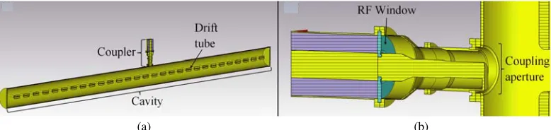
(a) (b)
Figure 1. The accelerating cavity of a typical DTL. (a) shows the entire resonant cavity with drift tubes and the portion of the coupler nearest the cavity. (b) shows the coupler geometry.
The test case is based on the 201.25 MHz DTL at the Los Alamos Neutron Science Center (LANSCE). An example of such a cavity is shown in Fig. 1. Such structures utilize standing electromagnetic (EM) waves to accelerate charged particles across the resonant cavity. These accelerating fields are established by coupling the cavity to the power source via a waveguide or transmission line. Outside of the cavity, only the portion of the coaxial transmission line nearest the resonant cavity needs to be considered since this will most accurately simulate the cavity response to the input. In order to prevent deceleration as the fields switch polarity, drift tubes are added along the beamline. Consequently, there is a high degree of complexity in the designed geometry of such structures, which are often on the order of ∼10 m long and ∼1 m in diameter.
In order for the DTL to reach steady state, the cavity must be typically driven by an input signal for a time of ∼ 0.1 ms. This long fill time is due to a number of factors, such as losses in the walls, the small percent of incident energy entering the cavity from the coupler, time for the summation of transient reflections to reach steady state, etc. Considering that the operation frequency is 201.25 MHz, the FDTD method for solving for the EM fields will require a time step on the order of 1–10 ps, as implied by (1). The large size of these structures (of > 10λ) and the high geometric complexity also means that there will be a large number (up to a few million) of points in the FDTD grid. Performing such simulations in parallel through two Intel XeonR E5-2650 v2 2.6 GHz processors, takes a week or two to achieve results corresponding to steady state. It is then desirable to develop a technique that reduces the simulation times.
The principle of our methodology utilizes a signal that is significantly larger than the nominal signal to reach the steady state conditions more quickly. The nominal signal, henceforth referred to as the long fill, is a constant amplitude, sinusoidal signal that is used in the practical operation of the DTL. For this work, the amplitude of the long fill was set to the nominal value of 1W1/2. The unit of
W1/2 comes from the interpretation of the input signal by our FDTD solver, as discussed in the next section. By increasing the amplitude of the long fill signal (by an amount calculated according to the next section) until some time t1 and then linearly decreasing the amplitude to that of the long fill, a
quick fill excitation is created. The quick fill consists of three regions: 1) Constant amplitude of P0
from time 0 to t1, 2) Linearly decreasing amplitude fromP0 to the nominal amplitude of 1 from times
Figure 2. Example of input power signal with the three distinct regions labeled. Region 1 has a high constant amplitude, Region 2 decreases this amplitude in a linear manner to the nominal values held in Region 3. Region 3 is representative of steady state. This signal has a frequency of 201.25 MHz, but witht1 and t2 set to much lower values so the sinusoidal nature is apparent.
should provide the same steady state EM fields as the long fill. Fig. 2 shows an example of the quick fill signal with these regions labeled. The selection of times t1 and t2 should be an order of magnitude
less than the fill time (∼100µs for a DTL), but still in the range of hundreds of periods, to ensure that any transient artifacts will be negligible.
2. GENERAL PROCEDURE
To validate the methodology of our approach and for comparison with the traditional methodologies, CST Microwave Studio was used. The formulation of the input signal requires knowledge of the resonant frequency of the mode to be analyzed, which was found by applying the FDTD solver to the specified frequency range of 200–350 MHz [8].
Our model incorporates one input/output port as shown in Fig. 3, so the resonant frequencies (f0) can be readily calculated from the peaks in the ratio of the output to the input at each frequency
(S-parameter). Once the f0 is established, the input signal needs to be determined. In order to reach
steady state with the long fill input, the signal must be run for a sufficiently long time. This time is the fill time and is on the order of ∼100µs for the DTL.
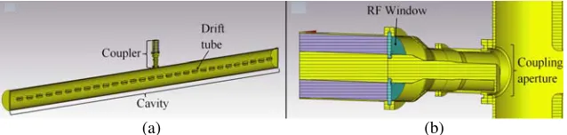
(a) (b)
Figure 3. The two perfect electrical conductor (PEC) cases used in verification of the proposed methodology. (a) shows the geometry used in cases A and B, while the geometry of case C is shown in (b). All cases used the radius of the DTL cavity at LANSCE. Cases A and B used a height that is approximately 1 λ, and the length of case C was selected to accommodate four drift tubes of 0.352 m in length with a center-to-center distance of 0.559 m between them. The rectangle at the top of the coupler is the only input/output port in the system.
The determination of the input amplitudes for the quick-fill case requires an analysis of the response of the cavity to an input signal. This response can be found by considering the following relation for the vector potentialA(r, t) of the field inside the cavity [9]:
∇2A(r, t)− 1
c2
∂2A(r, t)
where Jdr is the current density imposed by the input signal, and c and μ are the speed of light and magnetic permeability of the volume within the cavity. Further,
A(r, t) =qmode(t)Amode(r) (3)
whereqmodeis the time dependent portion of the particular mode, andAmodeis the spatially dependent portion.
The driving current density can be separated in time and space Jdr(r, t) = Jdr(t)J(r), because while J(r) is dependent upon the coupler geometry, Jdr(t) would be dependent upon the defined excitation signal. Jdr is considered to be directly proportional to the quick fill input Pin, so that
Jdr(r, t) =χPin(t)J(r), where χ is a constant with units of W−1/2, the signal Pin has units of W1/2, and bothJdr and J have the standard unit of A/m2. These units arise from how CST interprets input signals at a port with an impedance ofZ0, such that the voltage between the inner and outer conductor
and the current through the inner conductor areV =Pin √
Z0 and I =Pin/ √
Z0 respectively (the units
of I,V, and Z0 areA,V, and Ω) respectively). Consequently,
∂2qmode ∂t2 + 2α
∂qmode
∂t +ω
2
modeqmode=KPin(t) (4)
K=χ
V J(r)·Amode(r)dV
εV A2modedV . (5)
The complete derivation of (4) can be found in the appendix. Estimation ofαcan be done by using the full-width, half-max (Δf) of theS-parameter peak of the mode being analyzed through:
α= ω0 2Q, Q=
f0
Δf ⇒α=πΔf. (6)
The general solution to (4) for a signal of linearly varying amplitudeKPin = (mit+p0,i) sin(ωt) is
qmode,i(t) = (aicos(γt) +bisin(γt))e−αt+ (c1,it+c2,i) cos(ωt) + (c3,it+c4,i) sin(ωt), (7)
γ =
ω2
mode−α2 (8)
The subscript i in (7) indicates which of the regions (corresponding to Fig. 2) the variables correspond to. The calculation of the coefficients ai, bi, and ci is discussed in the appendix. Once ai,bi, andci have been determined fori= 1,2,3, the full response (qmode) of the cavity to a given input signal (KPin) is known.
The input KPin depends on three unknown parameters: t1, t2, and P0. The values for t1 and
t2 must be high enough that any transient artifacts from the EM fields propagating and reflecting off
cavity surfaces will be negligible. However, sincet2 is the target time after which the system is at steady
state,t2 should also be significantly lower than the time required for the long fill to reach steady state.
Beyond these two requirements, selection of t1 and t2 is arbitrary.
Oncet1 andt2 have been selected,P0 is found by applying different values ofP0 until the amplitude
of qmode is not changing by more than a defined tolerance of 10−8 (unitless) (see appendix) during the target steady state region. Two initial guesses for P0 are made, then subsequent guesses are found by
using the secant method [10]. The values used in the secant method areP0 and the average change of
the amplitude across the steady state region.
Once KPin is determined, the response of the system may now be evaluated. The validity of our approach was tested through a few test cases, which will be discussed next.
3. RESULTS AND DISCUSSION
The exact dimensions of the coupler, the coupling aperture, and the cavity radius were kept for the simulations, but to decrease the simulation time, the cavity height was changed as shown in Fig. 3.
The first case was (A) a cylindrical cavity made of a perfect electric conductor (PEC) with no drift tubes. This geometry is shown in the top portion of Fig. 3. At steady state, the input and output signals will have the same amplitude as each other. The loss that contributes toαis the power emitting back from the cavity through the aperture into the coupler.
The next test case (B) corresponded to a copper (non PEC) cavity with the same geometry as case A. A higherαwould be expected in this case due to the Ohmic resistance introduced in the cavity walls.
The last case (C) was a cavity with drift tubes added. PEC was selected as the cavity and drift tube material to remove the added complexity of Ohmic losses. This case was used to verify the overall validity of the approach with increased geometric complexity.
3.1. Cylindrical PEC Cavity
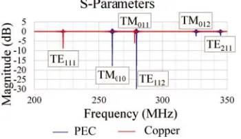
This test case was quick to simulate, and can also be modeled analytically, as discussed in the appendix. The specific geometry is found in Fig. 3. The radius corresponds to the cavity dimensions of the accelerator at LANSCE, and the height is about 1λ(∼4.969 m for 201.25 MHz). The frequency andα for this modified cavity were calculated from the S-parameter (only one value is necessary for the one port system) displayed in Fig. 4. These clearly show that the calculated resonant frequencies do in fact match the theoretical values obtained from the solution of Helmholtz Equation for a cylindrical cavity. The peak at 260.32 MHz was selected to be used for the demonstration of the quick-fill approach due to its correspondence to the fundamentalT M010 mode. This varies fromf0 = 201.25 MHz for the DTL
at LANSCE due to the changed geometry of the cavity.
Figure 4. S-parameter of cases A and B. The peaks closely match in frequency to each other and the theoretical values of the labeled modes. Losses in the walls of the copper cavity change the relative strength of these modes from the PEC cavity, resulting in the difference in peak depths.
The values for theα,Pin andf0 for this case and the other two cases are indicated in Table 1. The
robustness of the quick filling method can be displayed by using a variety of times for t1 and t2. The
value oft2 was selected to be an order of magnitude less than the time required for the long fill to reach
steady state (∼1/α). This allows the system to reach steady state more quickly while still allowing any possible transient artifacts from interfering with the results.
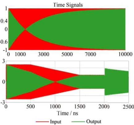
The long fill case was also run until steady was reached at around 10,500 ns and compared to the simulations from the quick filling case. Fig. 5 shows the input/output (I/O) signals from the long fill and quick fill cases. The following criteria indicate the quick fill gives the same results as the long fill case.
Figure 5. Input and output signals for the long fill (top) and quick fill (bottom) cases for the short PEC cavity. Both cases exhibit an initial decrease in output followed by an increase in output. The quick fill is able to achieve the same steady state output in 1,500 ns as opposed to 10,000 ns for the long fill. The input on the bottom portion is of the same shape as the signal in Fig. 2.
Figure 6. Voltage and current monitor locations along the coupler. The cavity is toward the right, with the monitors represented as grey arrows. The voltage monitors run from the inner to outer conductors, and the current monitors run in loops around the inner conductor.
The third criterion relates to the electric and magnetic field distributions within the coupler. For these simulations, voltage (V) and current (I) monitors were defined as shown in Fig. 6 The V will relate to the electric field distribution in the coupler, and I to the magnetic fields. Fig. 7 shows the respective distributions for both the long fill and quick fill cases. It is evident that the quick fill did successfully reach steady state because the profiles from the long and quick fill cases in Fig. 7 overlay exactly after 10µs and 1.5µs respectively.
3.2. Cylindrical Copper Cavity
This case was used to demonstrate that the quick-filling method is capable of filling a cavity made of lossy material. The values of α can be found in Table 1, and Fig. 4 illustrates that the S-parameter peaks for the copper cavity case were approximately the same in frequency but with different intensities. Because the strongest peak is now theT E111 mode at 222.855 MHz, this mode is analyzed in addition
to the peak at 260.322 MHz corresponding to theT M010 mode.
Figure 7 shows the voltage and current profiles for theT M010mode in both the PEC and the copper
Table 1. Parameters for various test cases of quick filling signals. An asterisk (*) indicates that the value forα was found using a least squares fit (11) of decay energy.
Case f0 (MHz) α(10−5 ns−1) P0(W1/2) t1 (ns) t2 (ns)
A(i) 260.322 49.11 2.44 50 1,950
A(ii) 260.322 49.11 4.55 250 750
A(iii) 260.322 49.11 2.54 500 1,500
B(i) 260.322 49.70* 5.86 500 1,500
B(ii) 222.855 15.32 7.00 500 1,500
C(i) 215.489 2.24 9.41 2,500 7,500
C(ii) 215.489 1.02* 20.14 2,500 7,500
Figure 7. Voltage and current profiles in the steady state for the long fill and quick fill cases for the T M010 mode in the short PEC and copper cavities. The voltage profiles have good agreement between
all cases. The current profiles show slightly higher values for the copper cavity.
Figure 8. I/O signals for the long fill (top) and quick fill (bottom) cases of the T E111 mode in the
copper cavity. The quick fill again reached steady state much more quickly than the long fill (1,500 ns vs. 35,000 ns).
The T E111 mode comparison between the long fill and quick fill inputs shows that the voltage
and current profiles have excellent agreement between the long and quick fill cases. Fig. 8 shows the I/O waveforms for the two inputs and indicates that the output strength (indicated in green on the plot) is of equal magnitude (≈0.96W1/2) for both the long fill and quick fill input waveforms. For the T E111 mode, steady state was reached in 35µs for the long fill case and in 1.5µs for the quick fill case.
Furthermore, the field energy of the system validates that the system did in fact reach steady state as the difference between the maximum and minimum energies over the target steady state region (relative to the maximum) is only 0.04 dB, or 0.917%.
3.3. Truncated PEC Cavity with Drift Tubes
The last case considered was that of a cavity with drift tubes as shown in Fig. 3. The coupler offset was selected to accurately model an actual DTL at LANSCE, and the height was selected to accommodate four drift tubes, representing a small segment of the DTL at LANSCE. This geometry results in resonant frequencies that are slightly lower than with the previous two cases, as indicated in Table 1. Fig. 3 shows this geometry. Because the T M010 peak was much weaker for the copper case (see Fig. 4), the
material for the cavity was selected to be PEC in order to ensure theS-parameters have a strong peak corresponding to this mode. PEC also implies that the output will be of equal magnitude to the input at steady state, giving us a way to check the validity of the approach without running the long fill, which would require >400µs to reach steady state.
The simulations did not result in the expected results that were observed for the previous cases. The amplitude of the output signal was about 10% that of the input, indicating that either α or ω0
must have been erroneously calculated if the quick fill method is to be valid for increased geometric complexity. These were calculated from theS-parameter, which is itself calculated by applying a Fourier transform to the time dependent I/O signals [8]. As theS-parameter calculations run, the energy, and thus the emitted power, of the modes that have been excited by the input signal decrease, leading to the S-parameter peaks changing in height but not frequency. This means thatαis likely to be miscalculated if the S-parameter calculations have not been run for a sufficient time. There is no method to predict the time for which the S-parameter calculations should be run, but this case ran for 50µs without producing reliable information to calculate α.
In order to accurately calculateα, a new method was considered. By using an input signal at the resonant frequency for a short time to partially fill the cavity, then bringing the input to zero, αcan be calculated from the emitted output after the input has been brought to zero. The length of time that the cavity is filled should be sufficiently long enough such that the majority of the field energy is in the cavity and not the coupler. Finding tf ill (not to be confused with the quick filling parameters t1 and
t2) can be difficult since α will still be unknown, but for this case we knew that it would have to be
∼1µs since the attempted quick fill of this cavity also required a time scale on the order of ∼1µs to achieve a partial fill. This quick fill information was not used to find α, however, because a standard procedure for calculating α needed to be tested. To calculate α, we used the definition of Q:
Q= 2πEnergy stored in cavity
Energy lost per cycle =−πf0 W ∂W
∂t
. (9)
The value ofα can be found to be:
α= ω
2Q =− 1 W
∂W
∂t . (10)
By solving this equation,
W(t) =Ce−αt, (11)
Figure 9. I/O signals (top) and relative field energy (bottom, in dB) of the partial fill used to calculate the attenuation coefficient. The inset plot of energy vs. time shows the data that is used to fit the parameters α and C in (11).
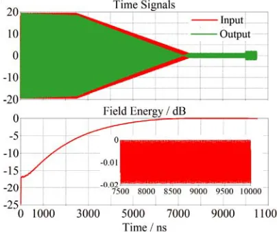
Figure 10. I/O signals (top) and relative field energy (bottom) of the quick fill for the PEC cavity with tubes usingα calculated from the decay energy. The field energy varies by 0.02 dB from the maximum during the steady state period between 7,500 ns and 10,000 ns.
α (CaseC(ii) in Table 1), the value of P0 was recalculated, and the simulation was run again with the
new input signal. This run showed the results that were expected, as seen in Fig. 10. The output signal and energy both show that steady state was reached. In order to reach the same variation of 0.02 dB (W/C = 0.0005) with respect to the maximum energy during the steady state of the quick filling signal, the long fill signal would have to run for 0.527 ms as calculated from (11).
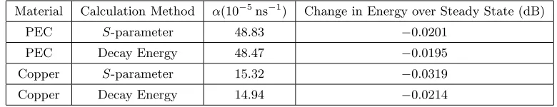
To ensure that this new approach for finding α is compatible with the previous two cases, α for those cases was re-calculated using the new method. A quick filling signal with times t1 and t2 set
Table 2. Recalculation ofαand its effect on the simulation of steady state. For PEC this was performed at 260.1978 MHz (T M010), and for copper at 222.296 MHz (T E111).
Material Calculation Method α(10−5ns−1) Change in Energy over Steady State (dB)
PEC S-parameter 48.83 −0.0201
PEC Decay Energy 48.47 −0.0195
Copper S-parameter 15.32 −0.0319
Copper Decay Energy 14.94 −0.0214
4. SUMMARY
The use of a carefully estimated input signal can allow for the quick and efficient simulation of highly resonant, electrically large systems, resulting in simulation that run in∼2 hours as opposed to 2 days or more. This procedure was compared, through CST based simulations, to three test cases aimed at understanding better the performance/optimization of a 201.25 MHz DTL at LANSCE.
Three cases, i.e., (A) cylindrical PEC cavity, (B) a cylindrical copper cavity, and (C) a cylindrical PEC cavity with drift tubes, were successively considered, and used to verify the validity of the approach. The work also necessitated the implementation of a new method for calculating an attenuation factor, α. This factor provides information about the time frame for a resonant structure to reach steady state, so by applying an input signal for a short time (i.e., until the emitted signal from the cavity is detectable), this method allowed α to be found for more complex geometries.
While the quick fill method was developed for the specific case of a DTL, extensions can be made into similar problems requiring information about the transition to steady state. The voltage and current profiles along the coupler indicate that the EM fields are accurately simulated, meaning that this method can be employed to investigate phenomena that require knowledge of the EM fields as the steady state of the system is reached. In particular, these phenomena, such as arcing or multipactor, require calculations of physical attributes other than the EM fields that add to the computation time. Such problems can benefit from the decreased simulation times without affecting the accuracy of the results.
APPENDIX A.
A.1. Derivation and Application of the Resonance Equation
The derivation of (4) from (2,3) requires that the spatially dependent portion of the modeAmode both satisfy the Helmholtz Equation and be orthogonal to other modes. Furthermore, using the definition of the Q-factor and its relation to an attenuation coefficient α, Q = 2πEnergy stored in cavityEnergy lost per cycle = 2ωα, we obtain:
∂2qmode ∂t2 + 2α
∂qmode
∂t +ω
2
modeqmode=
V J(r)·Amode(r)dV εV A2
modedV
. (A1)
By applying the particular solution qmode,particular,i(t) = (c1,it+c2,i) cos(ωt) + (c3,it+c4,i) sin(ωt)
to (4), the coefficients may then be determined through solving:
⎡ ⎢ ⎣
ω02−ω2 0 2αω 0
2α ω20−ω2 2ω 2αω
−2αω 0 ω20−ω2 0
−2ω −2αω 2α ω02−ω2
⎤ ⎥ ⎦ ⎛ ⎜ ⎝
c1,i c2,i c3,i c4,i
⎞ ⎟ ⎠= ⎛ ⎜ ⎝ 0 0 mi P0,i
⎞ ⎟
⎠ (A2)
For the other regions, the continuity of the values and time derivatives of qmode across regions is used to find the values of a and b by solving:
cos(γt) sin(γt) −αcos(γt)−γsin(γt) γcos(γt)−αsin(γt)
ai bi
e−αt=
q
mode,i−1(t)
qmode,i−1(t)
−
[c1,it+c2,i] cos(ωt) + [c3,it+c4,1] sin(ωt)
[c3,iωt+c1,i+c4,iω] cos(ωt)−[c1,iωt+c2,iω−c3,i] sin(ωt)
, i= 2,3 (A3)
For the nominal long fill signal, there is one region consisting of values m = 0 and P0 = 1. This
results in:
qmode(t) = 1 2ω
1
αcos(γt)− 1
γ sin(γt)
e−αt+ 1
2αωcos(ωt) (A4)
It is obvious from (??) that the magnitude at steady state will be 2αω1 . For the quick fill signal, the values for mi and P0,i are as follows:
m= ⎧ ⎪ ⎪ ⎪ ⎨ ⎪ ⎪ ⎪ ⎩ 0 1−P0
t2−t1
0
, p0=
⎧ ⎪ ⎪ ⎪ ⎨ ⎪ ⎪ ⎪ ⎩ P0
t2P0−t1
t2−t1
1
for
t < t1
t1≤t < t2
t≥t2
(A5)
The value of P0 is calculated for each set of geometries and times t1 and t2 by application of the
secant method to the average change in the peak values of qmode after time t2. Two initial guesses are
made for P0, and then the coefficients a, b, and c are calculated for each region to get the values of
qmode. Then the peaks of qmode after time t2 are determined, and the time derivative of these peaks is
calculated using finite difference formulas:
yn = [ yn−1 yn yn+1 ]
a b c n , (A6) ⎡ ⎢ ⎢ ⎢ ⎣ h0 n hn h2 n 2 ⎤ ⎥ ⎥ ⎥ ⎦ a b c n = 0 1 0 , (A7)
hn= [ tn−1 tn tn+1 ]. (A8)
whereyis a local peak value of qmode. This is then used to determine the average of the time derivative of the peak values over steady state ¯y. Subsequent values ofP0 are calculated using:
P0,n+1 =P0,n−y¯n
P0,n−P0,n−1
¯
yn−y¯n−1
(A9)
until ¯y is sufficiently close to zero. Considering the maximum amplitude for steady state from (??), a tolerance of <10−8 to 10−12 will give accurate values ofP0 for a large range of structures.
A.2. Modal Analysis of the PEC Cavity
The analytic model for modes in cylindrical coordinates gives the overall wavenumber as:
k2 =ω2με=kρ2+kz2 (A10)
where for TM modes:
k2ρ= χmn
r , Jm(χmn) = 0, k
2
z = pπ
and for TE modes:
k2ρ= χ mn r , J
m(χmn) = 0, kz2= pπ
h (A12)
where χmn is thenth zero of the Bessel function of the order mJm (distinct from the χ in Jdr(r, t) = χPin(t)J(r)), χmn is the nth zero of the derivative of the Bessel function of the order mJm , r is the radius, and h is the height of the cylinder. Solution of these parameters is summarized in Table A1.
Table A1. Calculation of the theoretical frequencies of the simple PEC cavity.
Type mn χmnorχmn p f (MHz)
TM 01 2.404826 0 260.30
TM 01 2.404826 1 278.26
TE 11 1.841184 1 222.24
TM 01 2.404826 2 326.27
TE 21 3.054237 1 344.91
TE 11 1.841184 1 280.02
REFERENCES
1. Liu, Q. H., “The PSTD algorithm: A time-domain method requiring only two cells per wavelength,” Microwave and Optical Technology Letters, Vol. 15, No. 3, 158–165, 1997.
2. Shaw, A. K. and K. Naishadham, “Efficient ARMA modeling of FDTD time sequences for microwave resonant structures,” IEEE Trans. Microwave Theory Tech., Microwave Symposium Digest, Vol. 1, 341–344, 1997.
3. Bondeson, A., T. Rylander, and P. Ingelstr¨om, Computational Electromagnetics, Springer, 2005. 4. Lee, T. W. and S. C. Hagness, “Pseudospectral time-domain methods for modeling optical wave
propagation in second-order nonlinear materials,” Journal of the Optical Society of America B, Vol. 21, No. 2, 2004.
5. Insepov, Z., J. Norem, et al., “Modeling RF breakdown arcs,” arXiv:1003.1736, 2011.
6. Kravchuk, L. V., G. V. Romanov, and S. G. Tarasov, “Multipactoring code for 3D accelerating structures,” arXiv:physics/0008015, 2000.
7. Cummings, K. A. and S. H. Risbud, “Dielectric materials for window applications,” Journal of Physics and Chemistry of Solids, Vol. 61, No. 4, 2000.
8. CST Studio Suite, CST, www.sct.com.
9. Wangler, T. P., RF Linear Accelerators, Wiley-VCH, 2008.