Analysis of Bistatic Scattering Due to Hydrometeors on SHF
and EHF Links in a Subtropical Location:
A Comparative Study Based on the Rain Cell Models
Pius Adewale Owolawi1, * and Tom Walingo2
Abstract—The inevitable increase in radio interference within microwave systems continue to be of major concern as more of radio communication services compete with bandwidth assigned to the fixed service, fixed satellite service and broadcasting satellite service. Interference hampers coverage and capacity of these services often lead to the reduction in the signal to noise ratio at the receiving terminals. The existing global hydrometeor scatter model proposed by the International Telecommunication Union when applied to the tropical and subtropical location often leads to considerable inaccuracies due to the wide range of intense climatic and geographical nature of this region. In this study, the bistatic intersystem interference due to hydrometeors between satellite systems and terrestrial downlink receiver terminal systems in a subtropical station computation is based on the Awaka and Capsoni cell models. For the attenuation of both wanted and unwanted paths to the receiver, the existing model based on the specific attenuation has been modified to include the equivalent path length through rain in the estimation of the attenuation. Results obtained show that the Capsoni model exhibits the normal trend under a moist atmosphere with a gaseous attenuation more pronounced at frequencies greater than or equal to 30 GHz. Also at high rain rates greater than 70 mm/h and considering the rain with melting layer, up to about 70 dB difference was observed between transmission losses estimated using Awaka and Capsoni models at link probabilities ranging between 1–10−3% unavailability of the time.
1. INTRODUCTION
The intersystem interference, which arises as a form of propagation impairment due to rain and other hydrometeors on microwave links, continues to draw attention of researchers all over the world. This is because more of radio communication services compete with the spectrum assigned to the fixed service (FS), fixed satellite service (FSS) and broadcasting satellite service (BSS). There is no gainsaying that the lower frequency bandwidth has been highly congested, and this has led to the adoption of frequency reuse whereby a terrestrial radio relay link will use the same frequency as that of the earth station link. This often results in co-channel interference. Co-channel interference, which arises due to the other carriers transmitted by the satellite to earth stations of the same system, at the same frequency and at the same polarization as the useful carrier, may be by legal or illegal means, and in spite of the International Telecommunication Union (ITU) recommendation based on the emitted power and frequency planning, this impairment continues to linger due to atmospheric factors among others most especially in the tropical and subtropical climates. In addition to the aforementioned factor, the rapid development of technology, as well as the increasing liberalization of telecommunications markets and the associated commercial pressures, also contributes to the problem of interferences.
Received 17 March 2015, Accepted 6 May 2015, Scheduled 1 June 2015 * Corresponding author: Pius Adewale Owolawi ([email protected]).
1 Department of Electrical Engineering, Mangosuthu University of Technology, Durban, South Africa. 2 Department of Electrical,
The effect of interference normally leads to a considerable signal-to-noise ratio (SNR) at the interfered terminal, and if not properly checked it might even result in the total outage of the desired receiving signal. It has been well affirmed that at frequencies greater than 10 GHz, a signal link (desired quality of the wanted channel) is subject to some negative consequences such as attenuation and scattering, depolarization, intersystem interference, among others, by precipitation particles along the radio path [1, 2]. For example, hydrometeor scatter is often the dominant mechanism for an Earth-station antenna pointed in the opposite general direction, while on interference paths between space and earth, hydrometeor scatter effects are almost always dominant [3]. Also, rain scattering is severe at these frequencies, because the size of the raindrop is comparable to the wavelength of the signal.
For interference to occur, the signal from the satellite intersects with the terrestrial signal at a region often referred to as the common volume in the rain height (0◦C isotherm height) where the radar reflectivity decreases to about 6.5 dB/km above it, resulting in strong ice-scattering and attenuation of the satellite channel [3]. The weak signal from the satellite is susceptible to severe interference from a strong terrestrial system operating in its neighborhood at the same frequency if the beam canters intersect and contain precipitating particles [4–6].
The impact of interference depends on path geometries, terminal separations, system parameters such as antenna directivity, frequency, and tolerance to interference, and local climatic factors. This impact hampers coverage and capacity, as well as limits the effectiveness of both new and existing communication satellite systems. Therefore, weighing the critical impact of such interference to the desired link on statistical bases, it is very crucial for planning engineers to undertake a number of interrelated but distinct tasks to correct the design of communication systems operating at SHF and EHF bands for optimum link performances.
The subject on the impact of interference studies has received much attention either by the direct measurement or by simulation mostly at the temperate region among which are the works of [1, 3, 7–11] to mention but a few. Also, the tropical region is not exempted with most of the work done in Nigeria by [2, 4–6, 12, 13].
Over the years, researchers have categorized subtropical alongside the tropical climate. However, studies show that there is a clear difference between the tropics and subtropics [14–16]. As per the Koppen climate classification, the tropical climate has high temperature and high humidity while a subtropical climate has high temperature and low humidity. In terms of storm, the tropical storms generate more rain than subtropical storms, with a typically very heavy thunderstorm activity in the subtropical when compared to a tropical storm. Rainfall is more of a stratiform type in the subtropical region than the tropical region which is more of a convective type [14, 15]. The specialty of these characteristics called for the investigation of the interference level being experienced when the signal is channeled in the subtropical rainfall, which this paper addresses among other things.
This paper adopts the simplified version of the improved Capsoni exponential rain cell model [10] to evaluate the impact of intense rainfall on the transmission signal in horizontally polarized SHF and EHF signal communication downlink in the subtropical environment based on thunderstorm rain types which predominate in the subtropical region, and the results obtained are compared with the Awaka 3D bistatic rain scatter model [8]. The bistatic radar equations were used along with single scattering theory and Rayleigh scattering for spherical droplets, to predict the bistatic system received signal levels. Our emphasis also focuses on the possibility of a terrestrial point-to-point microwave radio interfering with the reception of satellite traffics over both short (≤50 km) and long (>50 km) path lengths.
2. THEORETICAL DESCRIPTION OF RAIN SCATTER MODEL
Consider an electromagnetic energy radiated by a transmitting antenna and assume that this illuminates a region of space, which is intercepted by atmospheric precipitation. The result of the single scattering, based on the joint meteorological particles, may lead to transmission loss given by the Bistatic radar equation and can be expressed as [3, 17]:
1 L =
Pr
Pt =GtGr λ2 (4π)3
V c
Ft(ϑ1, φ1)Fr(ϑ2, φ2)At(R1)Ar(R2)Ag R12R22
dv
∞
0
N(D)σbis(i, o, D)dD (1)
Repeater Station Rain
Satellite Station Antennabeam width 1
Terrestrial Station
Aw
Pt
Pr
R1 R
2
Station separation
Common volume
Antennabeam width2 Satellite
Ls
LG
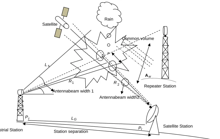
Figure 1. The scattering geometry between terrestrial station and an Earth satellite station as well as the additional rain attenuation,Aw on the path of satellite signal.
directivity function of the antenna systems, from which the effective areas are calculated. R1 and R2 are the path lengths from the transmitter and receiver to the common volume (Vc), respectively. At,r(R1,2) represents the attenuation along the paths from and towards the elementary volume, while Ag is the attenuation due to gaseous absorption. Gt,r are the transmitter and receiver antenna gains, while λis the wavelength of the radio signal and D is the particle equivolumic diameter. N(D) is the particle number density in a diameter interval, dD, while σbi is the total scattering cross-section of particles with diameter D inside the common volume, and it is related to the reflectivity factor, point rain rateR, and the complex refractive index of the raindrops.
Equation (1) can be further simplified to [18]:
1 L =
Pr Pt =
Vc
GtGrFt(ϑ1, φ1)Fr(ϑ2, φ2)At(r1)Ar(r2)Agσbi (4π)3R2
1R22
dv (2)
where every parameter retains its usual notation. The scattered wave arriving at the receiving antenna is composed of a very large number of elementary waves. Each elementary wave is generated from a single hydrometeor in the common volume. It can be assumed different from the others in size, shape, location and movement. In addition, all these elementary waves have undergone attenuation while traveling on slightly differing paths. Assume that the scattering process is through the single scattering pencil-beam width antenna approximation (PWAA). The scatter cross section per unit volume can be estimated through the complete Mie solution or Rayleigh approximation [3]. Hence, from the PWAA, Equation (2) takes the form:
1 L =
Pr Pt =
A1A2G1G2λ2Agσbi
(4π)3 xCv (3)
where the term Cv represents the common volume formed by the the intersection of the cones of the radiation patterns of the two antennas cut at the −18 dB level which is an integral part of the Equation (1) and is given as [18]:
Cv=
∞
0
F1(ϑ1, V1)F2(ϑ2V2) R21R22
all terms retain their usual notations. The quantities F1(ϑ1, V1) and F2(ϑ2, V2), which represent the directivity function of the transmitting and receiving antenna systems, are calculated in terms of their effective area. The relationship between the scattering cross section per unit volume,σbi, and the radar reflectivity, Z (mm6m−3), is:
σbi=10−18π 5
λ4 ε−1
ε+ 2
2Z(m2/m3) (5)
where εis the complex refractive index of the water, while the radar reflectivity, Z (mm6m−3), is the sum of the sixth powers of the diameters of all hydrometeors per unit volume and is related to the point rain rate, R, as:
Z = 10 logz (6)
where z = aRb and R is the rainfall rate (mm/h). The parameters ‘a’ and ‘b’ for the thunderstorm rainfall type based on the log normal rain drop size distribution proposed by [19] are used for this work. Therefore, in the dB scale and considering the contribution from the elementary volume forming the common volume and for practical applications, Equation (2) can be reexpressed by using the simplified bistatic radar equation (SBRE) as:
L=Pt−Pr =K+Ag−M+ (S−Z+A) (7)
All the terms in Equation (7) are in decibel (dB) units. M is the polarization decoupling factor, S the allowance for Rayleigh scattering at frequencies greater than 10 GHz, and K contains the linkage geometry and system parameters. A is the slant path rain attenuation from the transmitter to the common volume and from the common volume to the satellite receiver. In order to account for attenuation of both wanted and unwanted paths to the receiver, we therefore modify the existing model, which was based on the specific attenuation, by including an equivalent path length through rain in the estimation of the attenuation. The first step is to cater for the slant-path length,Ls, below the freezing rain height, Hr:
Ls= Hr−Hs
sinθ (km) (8)
whereθ is the slant path elevation angle and Hs the station height in km.
Table 1. Power law attenuation parameters for thunderstorm rain type [21].
Frequency kh αh
4 0.0003 1.0325 6 0.0032 1.0056 7 0.0046 1.0980 8 0.0043 1.3562 10 0.0175 1.1443 12 0.0285 1.1211 15 0.0476 1.0698 20 0.0998 1.0421 25 0.1356 1.0312 30 0.1161 1.0426 35 0.2002 0.9910 40 0.3234 0.9971 45 0.3967 0.9423 50 0.5284 0.8379 60 0.5830 0.8307
The ground projection,LG, of the slant path length is found from:
And a path length reduction formula meant for an exceedence value of 0.01% of time is introduced as [20]:
r0.01= 1
1 +LG(e0.015R0.01)/35 (10)
(For R0.01 > 100 mm/h, 100 mm/h is used instead of R0.01). The total slant path rain attenuation exceeds for 0.01% of time. A0.01 is then given by:
A0.01=γRLsr0.01 (11)
where γR is the specific attenuation (dB/km) and can be calculated using the power law relationship between rain rate and attenuation which is expressed as:
γR=khRαh (12)
The subscripthrefers to the horizontal polarization. The constant parameterskH andαH for calculating attenuation are shown in Table 1 for the frequencies investigated in this study and A for horizontally polarized signals only. The attenuation exceeded for some other time percentage, p (between 0.001% and 1%), is then obtained using the empirical scaling law [20]:
Ap =A0.010.12P−(0.546+0.043 log10P) (13) The structure of the rain along the path is very important for the evaluation of the statistics of transmission loss. A rain cell has been defined as any connected region of space composed of points where the rainfall rate exceeds a given intensity threshold [22]. The vertical structure of precipitation is assumed constant up to 0◦C isotherm height. Below this level is the rain region where attenuation and scattering of the wanted and the interfering signals occur. Beyond the 0◦C boundary, is the ice region whereZ decreases at the rate of 6.5 dB/km [9, 12]. The rain cell has a cylindrical symmetry within the horizontal cross-section, where the rainfall rate is assumed to vary exponentially at pointsxand y and can be expressed as:
R(x, y) =Rme−r/r0 (14)
whereris the radial distance with coordinate (x,y) from the rain cell centre, Rm the peak rainfall rate, and ro the parameter characterizing the cell size [1]. Equation (14) represents the statistical behavior of the rainfall rate profiles along a path, which are found to be able to reproduce the point rainfall rate cumulative distributionP(R) well enough [1, 5].
For Capsoni and Awaka rain cell models,ro is expressed respectively as:
ro(Rm) = 1.7
Rm 6
−10 +
Rm
6 −0.26
km (15)
ro(Rm) = 10−1.5 log10Rm lnRm
0.4
km (16)
Equations (15) and (16) differentiate the two models from each other. In order to give room for the differences in the rain cell from one location to another, the probability of occurrence of each cell in practice is represented by the cell spatial density. The probability of occurrence of a rain cell is defined in terms of the total number of rain cells N ∗(Rm) for a given area per unit rain rate R(r).
A general retrieval algorithm forN as proposed by Awaka can be expressed as
N∗(Rm) = −1 2πRmr2
o (RM)
dd3(lnP(RR))3
R=Rm
(17)
For the Capsoni model, the denominator of the first term on the right is two times higher [10].
A log-power law expression of Equations (16) and (17) was then adopted to define the measured values ofP(R) for 0< R < R. This is expressed as:
P(R) =Poln
R R
k
(18)
Table 2. Power law parameters for the local cumulative probability density for thunderstorm rain type for calculating transmission loss.
Location Coordinate Po R k
Durban, South Africa 29.58◦S, 30.57◦E 1.03×10⁻⁵ 484 12.8237
2.1. Methodology
2.1.1. Local Meteorological Parameters
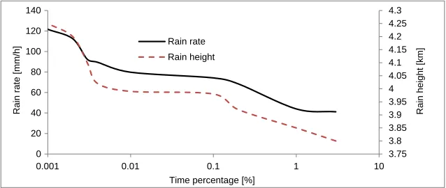
The location of the study is Durban (0.008 km, 29.58◦S, 30.57◦E), Kwazulu Natal Province of South Africa. For the purpose of this work, we have adopted the subtropical lognormal raindrop size distribution proposed by [15] as applicable to the subtropical stations. We also adopted the Z-R relationship proposed by [19] for thunderstorm rain based on lognormal fit in order to deduce the distribution fit for the convective thunderstorm rain type. The frequency range between 4 and 40 GHz (C-Q/V band) used presently by most service providers for terrestrial and Earth-space communications was considered. The mean annual cumulative distribution of point rain rate P(R) measured at Durban [14] was also used to predict interference levels with the availability probability ranging from 99–99.999%. The attenuation of the signals due to rain was evaluated using the Power law relationship between attenuation and rain rate, while an average water vapour density of 20 g/m3 was assumed to calculate attenuation due to atmospheric gases using the parameters in [23]. Water temperature of 20◦C was also assumed to calculate the refractive index of water using the method of [24]. The 0◦C isotherm heights during rainy conditions,hF R, vary from 3.80–4.25 km in South Africa as obtained from the South African Weather Station (SAWS).
2.1.2. Geometry and Electrical Characteristics of the Link
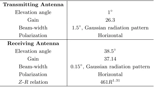
Intersystem interference produced at the input of the received Earth station, by carriers transmitted by the Intelsat IS-17 a geostationary (Geo) satellite located at 66◦ Een-route Durban is considered. Geo satellite has been known to offer a 24 hour view of a particular area, which leads to its wide use as a provider for broadcast satellite services (BSS) and multipoint applications. Although, under an ideal system these carriers should be strongly attenuated, due to multiplex schemes, frequency and polarization plans, antenna patterns and filtering issues. Several of the geometrical and electrical parameters are considered in this study as a result of interference caused by rain and melting-snow. The parameters are summarized in Table 3.
3. RESULTS AND DISCUSSION
The modified form of the bistatic radar Equation [10] and the exponential rain cell model of [1] have been employed to predict the cumulative distribution of transmission loss, L, for propagation paths
Table 3. The geometric and electrical properties of the link [25].
Transmitting Antenna
Elevation angle 1◦
Gain 26.3
Beam-width 1.5◦, Gaussian radiation pattern Polarization Horizontal
Receiving Antenna
Elevation angle 38.5◦
Gain 37.14
Beam-width 0.15◦, Gaussian radiation pattern Polarization Horizontal
in Durban, South Africa, and the results have been compared with the modified Awaka 3D rain cell model. The two models have been subjected to the same modification as stated in Section 2. Several scenarios were investigated to study the behavior of rain-induced bistatic scattering at SHF and EHF bands. This analysis was performed to determine the general behavior in the case of link configurations not experimentally measured. Figure 2 presents the distributions of rainfall rate and rain height used in the calculations to show the general behavior in the case of link configurations at different time unavailability considered in this work. Rain height is the height of the column above mean sea level. The result shows that rain rate decreases linearly with rain height over the average length of time a given threshold of rain rate or rain height is exceeded (signal outage time). This may be due to the fact that higher rain rate is associated with large rain cell diameter, and it could be strengthened by the convective upthrust at higher rain height. As the rain rate decreases so does the rain height due to the stratiform downward thrust. Although not discussed here, this invariability leads to break point as earlier observed by [26].
3.75 3.8 3.85 3.9 3.95 4 4.05 4.1 4.15 4.2 4.25 4.3
0 20 40 60 80 100 120 140
0.001 0.01 0.1 1 10
Rain height [km]
Rain rate [mm/h]
Time percentage [%] Rain rate
Rain height
Figure 2. Cumulative distributions of rainfall rate and rain height used for the simulation.
3.1. Comparison of Common Volume (CV) with Antenna Station Separation
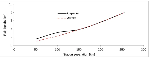
Figure 3 presents the equivalent satellite to common volume distance and the corresponding station separation. The common volume is calculated by integrating Equation (4) using a three dimensional Simpson integration algorithm. This is calculated once and for all, for all geometry irrespective of the other input parameters, and the extent of the rain cells. The result shows that the common volume, Cv, calculated using the two models increases linearly as station separation increase. The linearity is more pronounced with the Awaka model compared with the Capsoni model. At station separation less than 150 km, there is a difference of about 1 km between the two models, which may be due to the fact that the Awaka model initially does not include gaseous attenuation.
At station separation longer than about 150 km, the common volume will be in the ice region (rain height ∼3.9 km) as depicted in Figure 3, where ice scattering is dominant. In this case, the Cv will be above rain height and subjected to a considerably higher interference than when it is below the rain height. This scenario differs a little from the result for the tropical region and is noticeable at station separation, longer than about 170 km [2].
3.2. Transmission Loss Based on Different Models
0 50 100 150 200 250 300
Station separation [km] Capsoni
Awaka
0 2 4 6 8 10
Rain height [km]
Figure 3. Comparison between common volume distance and the corresponding station separation
distance.
110 120 130 140 150 160 170
0.001 0.01 0.1 1 10
Transmission loss [dB]
Time percentage [%]
Capsoni model ITU-R model Awaka model Frequency = 25 GHz, path = 200 km
Frequency= 12, path = 50km
Figure 4. Comparison of transmission loss between the two models and the ITU model over frequencies 12 and 25 GHz at short and long path lengths respectively.
However, the reverse is the case when a short path length is considered. The result shows that the ITU model underestimates the interference compared to the two models. This might be due to the fact that the data from this region were not included in the ITU-R rainfall model [27] because of insufficient long-term experimental data and scarcity of deployed equipment. Hence a regional classification is adopted which grossly underestimates the real-time measurement obtained from this region [14].
Figure 5 presents a comparison of interference from the melting layer, as a function of convective rain rate, at 12 GHz for the geometry of the 50 km, using the two models. The calculations for a melting layer was based on the rain height within the common volume where scattering and attenuation dominates the core rain cell and assuming only attenuation in the exponential cell surrounding the common volume. The melting layer calculation has been based on the method used by [9] with theZ-R relation in the rain just below the melting layer to point rain rate R on the ground as 461R1.31 [18]. Scattering cross sections and attenuations for the assumed water-related snow spheres were obtained as discussed earlier in Section 2. The results show that when rain with melting layer was considered, the transmission loss value obtained was less (indicating a higher value of interference at the receiver terminal) than when rain alone was considered. It has earlier been suggested by [28] that melting layer scatter should be taken into account in both coordination-contour and detailed-interference calculations for frequencies in and below the 11–14 GHz band. However, at high rain rate greater than 70 mm/h and considering the rain with melting layer, we observed up to about 10 dB between interference estimated using the Awaka and Capsoni model.
3.3. Influence of Frequency
80 90 100 110 120 130 140
20 40 60 80 100 120 140
Transmission loss [dB]
Convective rain rate [mm/h]
Awaka model
Capsoni model
Rain with melting layer Rain alone
Figure 5. Comparison of transmission loss with and without the melting layer as a function of rain rate at 12 GHz.
125 130 135 140 145 150 155
0 5 10 15 20 25 30 35 40 45
Transmission loss [dB]
Frequency [GHz]
Awaka Model
Capsoni model
50 km 200 km
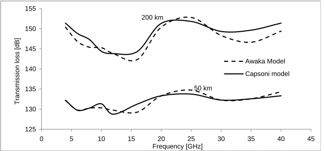
Figure 6. Comparison of the frequency characteristics of the transmission loss for the two models at 0.01% of time, for both short and long path lengths.
in transmission loss at frequencies≤10 GHz and path lengths of 200 km, but arises thereafter up to the frequencies ≤ 16 GHz for the two models. At frequencies greater than 20 GHz, the transmission loss is significantly higher in the earth station receiver terminal than at other frequencies with the peak at around 22 GHz, but then decreases to a minimum near 30 GHz as pointed out in [29]. This scenario might be due to the presence of gaseous attenuation in the moist atmosphere at such path lengths. It may also be due to the strong path length attenuation as well as the rapidly decreasing radar reflectivity in the ice region at 200 km. In all the frequencies considered at 99.99% availability of time, there is a slight difference of about 1 dB between the models mostly at a path length>200 km.
The results of variation of the transmission loss with % of the time, terrestrial antenna to common volume distance of 50 and 200 km (short and long path length respectively) and varying the frequencies (Figure 7) show that at availability time less than 99.9% (0.1% unavailability), the Awaka model produced less transmission loss when compared with the Capsoni model. The difference between transmission losses estimated using Capsoni and Awaka models ranges between 126 to 135 dB and 128 to 136 dB at 16 and 30 GHz respectively, for short path length (50 km), and from about 138 to 149 dB and 144 to 153 dB at 16 and 30 GHz, respectively, when the path length is 200 km and for the link unavailability between 3 and 0.001% of the time.
3.4. Varying the Terrestrial Propagation Path Length
120 125 130 135 140 145 150 155
0.001 0.01 0.1 1 10
Transmission loss [dB]
Timepercentage [%]
Awaka model
Capsoni model 16 GHz
30 GHz
16 GHz 30 GHz
200 km
50 km
Figure 7. Comparison of the transmission loss with % of the time, terrestrial antenna to common
volume distance of 50 and 200 km (long path length) and varying the frequencies.
120 130 140 150 160 170 180 190 200
0 50 100 150 200 250 300
Transmission loss [dB]
Terrestrial station to common volume distance [km] 12 GHz-Capsoni model
20 GHz-Capsoni model 30 GHz-Capsoni model 12 GHz-Awaka model 20 GHz-Awaka model 30 GHz-Awaka model
Figure 8. Variation of the transmission loss with terrestrial antenna station to common volume distance of 50 km (short path length) and frequencies 12, 20 and 30 GHz at 0.01% unavailability of time.
of time there is a gradual increase in transmission loss as station separation increases.
The results further show thatLis higher at frequencies 20 GHz than at other frequencies considered at a path length greater than 150 km due to the effect of gaseous attenuation in the moist atmosphere as well as a strong path length factor. Further, at a distance of about 100 km and frequency of 30 GHz, the difference between estimatedL using Capsoni and Awaka is about 5 dB for the same probability of 0.01%. This difference decreases as the distance between the TS-CV increases.
Figure 9 is for a frequency of 16 GHz, TS-CV distance of 50–250 km, and for the ease of presentation, we considered the percentage probability ranging from 0.01% to 0.1%. Generally speaking, Lincreased with increasing terrestrial (TS) to common volume (CV) distance (or terrestrial to satellite antenna separations, Tx-Rx). At TS-CV distance of 50 km (Tx-Rx of 50.7 km) and time probability of 0.01%, L is about 131 dB and 129 dB, respectively, using Capsoni and Awaka models (about 1.5% difference). At the time percentage of 0.1, the value was about 2 dB difference between the two models considering the same attenuation. We also observed that the shorter theTS-CV (the closer the stations) was, the higher the interference received in the satellite channel was since the interfering signal arrived weaker due to its increased path attenuation.
3.5. Influence of Terrestrial Antenna Gain
120 125 130 135 140 145 150 155 160 165
0 50 100 150 200 250 300
Transmission loss [dB]
Terrestrial station to common volume distance [km] Capsoni model
Awaka model
0.1 %
0.01 %
Figure 9. Comparison of the cumulative distribution of transmission loss with TS-CV at varying
percentages of time and frequency 16 GHz.
110 115 120 125 130 135 140 145 150
38 40 42 44 46 48 50 52
Transmission loss [dB]
Terrestrial Antenna Gain [dB]
Capsoni model
Awaka model TS-CV = 200 km
TS-CV =50 km
Figure 10. Influence of the cumulative distribution of transmission loss with terrestrial antenna gain over station separation of 50 and 200 km at frequency 12 GHz and varying percentages of time.
while at long path length, there seems not to be a difference between the two models. Hence, the Awaka model predicts a low interference at various antenna gains for these percentages of time at short path lengths. The same was observed in the tropical region in the work of [6].
4. CONCLUSION
5 dB at the same link unavailability probability of 0.01% (equivalent to about 5.3 hrs per year). This difference decreases as the distance between the TS-CV increases. This kind of difference in dB could not be overlooked in link budgeting-design since it could lead to under or overestimation of interference level prediction and, if not properly handled, could result in link outages which might grossly affect customer service interest in this location. Therefore, it may be concluded that the modified Capsoni model is recommended to be used for estimating interference due to hydrometeors in the Subtropical region.
REFERENCES
1. Capsoni, C., F. Fedi, C. Magistroni, A. Pawlina, and A. Paraboni, “Data and theory for a new model of the horizontal structure of rain cells for propagation applications,”Radio Science, Vol. 22, No. 3, 395–404, 1987.
2. Ojo, J. S. and R. C. Okeowo, “The application of 3D rain scatter model on horizontally polarized shf signal propagation in tropical location,”Int. J. of Infrared Millimeter Waves, Vol. 29, 1136–1145, 2008.
3. Crane, R., “Bistatic scatter from rain,” IEEE Trans. Antennas and Propagation, Vol. 22, No. 2, 12–320, 1974.
4. Ajewole, M. O. and J. S. Ojo, “Intersystem interference due to hydrometeor scattering on satellite downlink signals in tropical locations,”African Journal of Science and Technology (AJST) Science and Engineering Series, Vol. 6, No. 2, 84–89, 2005.
5. Ojo, J. S., S. K. Sarkar, and A. T. Adediji, “Intersystem interference on horizontally polarized radio signals in tropical climate,” Indian Journal of radio and Space Physics, Vol. 37, 408–413, 2008. 6. Ojo, J. S. and C. I. Joseph-Ojo, “An estimate of interference effect on horizontally polarized
signal transmission in the tropical locations: A comparison of rain-cell models,” Progress In Electromagnetics Research C, Vol. 6, 67–79, 2008.
7. Doherty, L. H. and S. A. Stone, “Forward scatter from rain,” IEEE Trans. Antennas Propagation, Vol. 8, No. 4, 414–418, 1960.
8. Awaka, J., “A 3D rain cell model for the study of interference due to hydrometeor scattering,” J. Comm. Res. Lab., Vol. 36, No. 147, 13–44, 1989.
9. Olsen, R. L., D. V. Rogers, R. A. Hulays, and M. M. Z. Kharadly, “Interference due to hydrometeor scatter on satellite communication links,”Proc. IEEE, Vol. 81, No. 6, 914–922, 1993.
10. Capsoni, C. and M. D’Amico, “A physically based simple prediction method for scattering interference,” Radio Sci., Vol. 32, No. 2, 397–407, 1997.
11. CakajShkelzen, K. and A. L. Scholtz, “Modelling of interference caused by uplink signal for low Earth orbiting satellite ground stations,” Proceedings of the 17th IASTED Int. Conference on Applied Simulation and Modeling, 187–191, Corfu, Greece, 2008.
12. Ajewole, M. O., L. B. Kolawole, and G. O. Ajayi, “Evaluation of bistatic intersystem interference due to scattering by hydrometeors on tropical paths,”Int. J. of Satell. Commun., Vol. 17, 337–356, 1999.
13. Ajewole, M. O., “Bistatic interference due to tropical rainfall types: A comparison of rain-cell models,” Attidella Fondazione Giorgio Ronchi, Vol. 58, No. 1, 121–141, 2003.
14. Owolawi, P. A., M. O. Fashuyi, and T. J. Afullo, “Rainfall rate modeling for LOS radio systems in South Africa,”SAIEE Transactions, African Research Journal, Vol. 97, No. 1, 2006.
15. Owolawi, P., “Raindrop size distribution model for the prediction of rain attenuation in Durban,” PIERS Proceedings, 1068–1075, Suzhou, China, Sep. 12–16, 2011.
16. Alonge, A. A. and T. J. Afullo, “Seasonal analysis and prediction of rainfall effects in eastern South Africa at microwave frequencies,”Progress In Electromagnetics Research B, Vol. 40, 279–303, 2012. 17. Kerr, D. E., Propagation of Short Radio Waves, Sect 2:1, Mc Graw Hill, New York, 1951.
19. Ajayi, G. O. and I. E. Owolabi, “Rainfall parameters from disdrometer dropsize measurements at a tropical station,” Ann. Telecomm., Vol. 42, Nos. 1–2, 3–12, 1987.
20. Glover, I. A. and P. M. Grant, Digital Communication, 3rd edition, Pearson Education Ltd., Edinburgh Gate, Harlow, England, 2010.
21. Owolawi, P. A. and S. J. Malinga, “Computation of rain scattering properties at SHF and EHF for radio wave propagation in South Africa,” Presented at URSI 2013, Ottawa, Ontario, Canada, 2013.
22. Commission of the European Communities on Cooperation in the Fields of Scientific and Technical Research, COST Project 210 Campaign, Final Rept. EUR 13407EN-C, ISBN 92-826-2400-5, Brussels, 1991.
23. ITU-R, Rec. P.836-5, “Water vapour surface density and total columnar content,” ITU Geneva, 2013.
24. Ray, R. S., “Broadband complex refractive indices of ice and water,” Appl. Opt., Vol. 11, No. 8, 1811–1836, 1972.
25. http://www.satellite-calculations.com/Satellite/Downlink.htm.
26. Bryant, G. H., I. Adimula, C. Riva, and G. Brusaard, “Rain attenuation statistics from rain cell diameters and heights,” Int. J. Satell. Commun., Vol. 19, 263–283, 2001.
27. ITU-R Rec. P.837-6, “Characteristics of precipitation for propagation modelling,” ITU-R, Geneva, 2012.
28. Thurai, M. and J. W. F. Goddard, “Precipitation scatter measurements from a transhorizon experiment at 11.2 GHz,”IEE-Proc.-H., Vol. 139, 53–58, 1992.
![Table 1. Power law attenuation parameters for thunderstorm rain type [21].](https://thumb-us.123doks.com/thumbv2/123dok_us/1988895.1263085/4.612.238.376.486.697/table-power-law-attenuation-parameters-thunderstorm-rain-type.webp)