AN ADAPTIVE REDUCED RANK STAP SELECTION WITH STAGGERED PRF, EFFECT OF ARRAY DIMEN-SIONALITY
B. A¨ıssa
EMP
B. P. 17, Bordj El Bahri, Algiers, Algeria M. Barkat
American University of Sharjah Sharjah, UAE
B. Atrouz
EMP
B. P. 17, Bordj El Bahri, Algiers, Algeria M. C. E. Yagoub
SITE, University of Ottawa Ottawa, Canada
M. A. Habib
EMP
B. P. 17, Bordj El Bahri, Algiers, Algeria
Abstract—Space-Time Adaptive Processing (STAP) is a well known technique in the area of airborne radars, which is used to detect weak target returns embedded in strong ground Clutter, Jammers, and receiver Noise. STAP has the unique property of compensating for the platform motion induced Doppler spread, thus making detection of slow targets possible. But there are other problems resulting from the characteristics of the airborne radar that may limit the performance of detection of the radar, for instance, the ambiguities (Range or Doppler ambiguities) which are dependent on the value of the pulse repetition frequency (PRF). When PRF is high, range ambiguities appear; when
PRF is small, Doppler ambiguities appear; and both are present when PRF is medium. To resolve Doppler ambiguities staggering of PRF is used. And to resolve problem of high computational cost of optimal space-time processing, reduced-rank methods are used. In this paper, STAP processing on the airborne radar is briefly reviewed for motivation, and the effect of a radar parameter dimensionality set on the STAP and the Reduced-Rank STAP is discussed.
1. INTRODUCTION
Radar detection has opened new interesting research fields in both military and civil contexts [1–6]. Signal detection using an array of sensors has offered significant benefits in a variety of applications such as radar, sonar, satellite communications, and seismic systems. Employing an array of sensors overcomes the directivity and beam width limitations of a single sensor. Additional gain afforded by an array of sensors leads to improvement in the Signal-to-Noise-ratio, resulting in an ability to place deep nulls in the direction of interfering signals. Finally, a system using an array of sensors affords enhanced reliability compared to a single sensor system. For example, sensor failure in a single sensor system leads to severe degradation in performance whereas sensor failure in an array results in graceful performance degradation. An adaptive detector for possibly range-spread targets has been considered by many authors [7–12].
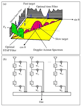
In practice, the interference statistics, interference spectral characteristics, and target complex amplitude are unknown. Thus, the problem of adaptive radar target detection in interference is equivalent to the problem of statistical hypothesis testing in the presence of nuisance parameters. Actually, computing power permits the use of well-known tools from statistical detection and estimation theory in the radar problem. The Doppler-Wavenumber or angle Doppler spectrum provides a unique representation of a signal in a three dimensional plane. Hence, the problem of space-time adaptive processing (STAP) may also be viewed as a spectrum estimation problem where the two-dimensional Fourier transform of spatio-temporal data affords separation of the desired target from interference. This scenario is described in Figure 1.
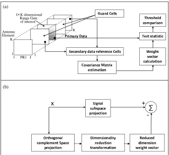
time dimensions, especially for detecting slow-moving targets [13–15]. The data collected by STAP radars can be viewed as a sequence, in range, of “N s×N t” (2D) arrays, which can be viewed as matrices, but are generally, treated as “N sN t×1” (1D) vectors. These array matrices or vectors are called “snapshots”. Each snapshot corresponds to a specific range. The optimum STAP processor computes the optimum weighted linear combination of the snapshot elements to determine if a hypothetical target is present or not. This calculation generally involves the estimation and the subsequent inversion of the “N sN t ×N sN t” covariance matrix (CM) of interference-plus-noise (I +N) snapshots. Furthermore, the array geometry introduces an element-to-element spatial correlation as shown in Figure 2. Thus in the context of STAP, the unknown interference spectral characteristics correspond to the unknown spatio-temporal correlation or covariance matrix of theIN×1 complex-vector under the condition that the data consists of interference alone. The estimation of the CM at any given range is typically performed using snapshots at neighbouring ranges (Figure 2). However, there are two major reasons that the optimum processor (OP) cannot be used in practice, first, (i) the inversion of the “I+N” CM requires on the order of “(N sN t)3” operations, which can be prohibitive for real-time applications, and second, (ii) the number of training snapshots needed to estimate the CM is between “2N sN t” and “5N sN t”. For typical values of “N s” and “N t”, this amount of data is most probably not available. These two problems have motivated the design of what we call “suboptimum methods (SOMs)” that reduce the size of the CM. Such methods lead to a drastic reduction of the computational cost and of the number of training snapshots required. To resolve Doppler ambiguities, staggering of PRF is used. And to resolve problem of high computational cost of optimal space-time processing, reduced-rank methods are used (Figure 2(b)). In this paper, the effect of a radar parameter dimensionality on the space time adaptive processing and the reduced rank adaptive processing on the airborne radar and the staggered PRF on the Reduced-Rank STAP performance is discussed.
2. DATA MODELS
information. The snapshot is stacked column-wise to form a KJ ×1 vectorX.
(a)
(b)
z-1
z-1
z-1
z-1
z-1
z-1 w11
w12
w1J w2J
Σ
Out
wKJ z-1
z-1 w22
z-1 w K1
wK2 w21
sin θ
Slow target
Doppler Azimut Spectrum cos θ
Fast target
Optimal time Filter
Optimal STAP Filter
Fd
Optimal Space Filter
Figure 1. (a) Space (angle)-time (Doppler) domain, (b) STAP architecture.
Under the signal-absence hypothesis H0, the data vector X
consists of clutter, Jammers, and noise components only, i.e.,
X =Xc+Xj+Xn=n (1)
where Xc, Xj, and Xn represent the ground clutter, jammers, and
vector, i.e.,
X=αS+n (2)
whereα=|α|ejφ is a complex gain whose random phaseφis uniformly
distributed between 0 and 2π, andSthe signal steering vector defined as follows:
S =St⊗Ss (3)
where⊗represents the Kronecker product, andSs∈CK andSt∈CJ
are the spatial and temporal steering vectors respectively. Denoting
Fs=
dsinθd
λ , Ft=fdTr (4)
As the spatial and normalized Doppler frequencies of the target signal,
(a)
(b)
J K dimensional× Range Gate
of interest
Antenna Element K
R
1
1 PR1 J 1
respectively,
Ss =
1
e−j2πFs
e−j2π2Fs .. .
e−j2π(K−1)Fs
, St=
1
e−j2πFt
e−j2π2Ft .. .
e−j2π(J−1)F t (5)
whereTr is the PRI and is equal to the inverse of the PRF andθdand
fdare the angle and Doppler, respectively, of the desired look direction.
Covariance matrix: The space-time covariance matrix is defined as
R =EnnH =Rc+Rj +Rn (6)
where Rc, Rj and Rn are the covariance matrices of the clutter,
Jammers, and noise, respectively.
Receiver noise: Thermal noise is assumed white across the array and over the frequency band of interest. Stated another way, sensor outputs are uncorrelated to each other and uncorrelated to themselves. The resulting covariance matrix is the unity matrix scaled by the noise power
Rn=σ2I (7)
It should be noted, however, that when the covariance matrix is estimated from the data, the noise covariance matrix will not necessarily have the form shown in Equation (7).
Clutter: The clutter extends over a sector of angles, and due to the flight geometry of the airborne radar, it covers a band of Doppler frequencies. It is assumed that the clutter can be adequately approximated by dividing the angular region corresponding to the range of interest into patches and computing the return from each patch. The return from each clutter patch is similar to the return from the target. Therefore, the clutter covariance matrix is given by
Rc =
NC
k=1
ξStkStkH
⊗SskSskH
(8)
whereξis the clutter-to-noise ratio (CNR);Ncis the number of clutter
patches, andSsk andStk are the spatial and temporal steering vectors,
respectively, of thekth clutter patch.
is uncorrelated and that the jammers are independent, the jammer covariance matrix is given by:
Rj = J
i=1
J
j=1
αiαHj ⊗SsiSsjH =AEAH (9)
where
A = [Ss1, Ss2, . . . , SsJ] (10)
E = diag
σ2ξ1, σ2ξ2, . . . , σ2ξJ
(11) And
αi =
αi0, αi1, . . . , αi(K−1) (12)
is the random amplitude vector of theith barrage noise jammer, and
ξi is its jammer-to-noise ratio (JNR).
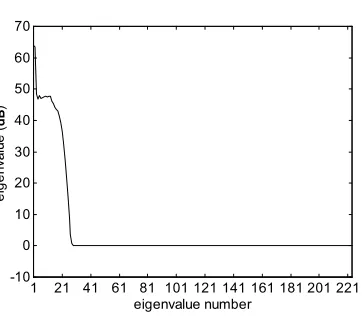
The eigenanalysis of the space-time covariance matrix reveals a few large eigenvalues and a large number of small eigenvalues. The number of large (principal) eigenvalues is predicted by the Landau-Pollak Theorem [16]. The theorem states that the system energy is essentially concentrated on its largestr= 2BTr+ 1 eigenvalues, where
B is the bandwidth covered by the signals received by the array and
Tr is the total duration of those signals across the array structure.
3. REDUCED-RANK PROCESSING WITH KNOWN COVARIANCE
The objective of partially adaptive STAP is to break one large adaptive problem into several smaller adaptive problems while still achieving close to optimum performance. This is possible since, as stated before, the interference covariance matrix is not of full rank. Partially adaptive STAP algorithms start by transforming the data with aKJ×r matrix
V. Studies by many authors (e.g., Ward [17], Haimovich [16]) have been concerned with subspace techniques to reduce the computational load while approximating the clutter rejection performance of the optimum processor to the greatest extent. The number of significant clutter eigenvalues indicates the minimum number of degrees of freedom (or, equivalently, the dimension of the clutter subspace) required for effective clutter rejection. Figure 3 shows a typical eigenspectrum for a sidelooking array.
dB
Figure 3. Eigenvalues of space-time covariance matrix.
maximize the output SINR. The full dimension (i.e., withoutV) weight vector of the direct form processor is given by
W =R−1S (13)
And theRR weight vector by
W =VHRV−1VHS (14)
The SINR equation for the full dimension direct form processor is [18]:
SINRopt=|α|2SHR−1S=|α|2
KJ
i=1
fiHS2
λi
(15) where{fi}KJi=1 are the eigenvectors ofR and{λi}KJi=1 are the associated
eigenvalues. With theRRweight vector defined as in (14), the output SINR for the RR direct form processor is given by [19]:
SINRRR=|α|2SHV
VHRV−1VHS (16)
Now, if we restricted ther columns ofV be a unique subset of the eigenvectors ofR, then we can rewrite (16) as:
SINRRR =α2SHVΛ˜−1VHS =α2 r
i=1
vHi S2
λi
(17)
where ˜Λ is a diagonal matrix of the eigenvalues associated with the r
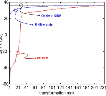
3.1. Principal-Components Method (PC)
The PC method (also known as the eigencanceler method [19]), as its name implies, refers to the retention of only those eigenvectors of the interference-only covariance matrix with corresponding eigenvalues of significant magnitude.
For the DFP, the PC method retains ther dominant eigenvectors of the full interference covariance matrix R. The resulting PC-based DFP weight vector W =WP C−DF P has the form:
WP C−DF P =S− r
i=1
λi−λmin
λi
fiHSfi (18)
whereλ1≥λ2 ≥. . .≥λKJ.
The rank-reducing transformation, V ∈ CKJ×r is again of the form
V = [f1 f2 . . . fr]. (19)
40
20
0
-20
-40
-60
-80
SINR (dB)
0 50 100 150 200 250 300 350 400
Rank
SINRopt
PC
Figure 4. Output SINR DFP-PC performances as function of rank.
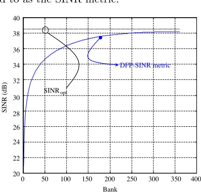
3.2. SINR Metric Method
partial sum is maximized by selecting the r columns of V to be the eigenvectors which maximize the quantity [20]
fH
i S
2
λi
(20) This is referred to as the SINR metric.
Bank 40
38
36
34
32
30
28
26
24
22
20
SINR (dB)
SINRopt
DFP-SINR metric
0 50 100 150 200 250 300 350 400
Figure 5. Output SINR DFP-metric performances as function of rank.
4. IMPROVEMENT FACTOR AND STAGGERED PRF
4.1. Improvement Factor
The system performance of the processor can be exhibited by the Improvement Factor (IF) when the ground clutter is assumed to be Gaussian random distribution. TheIFis defined as the ratio of output of the signal and interference-plus-noise ratio (SINR) against input SINR. The optimum improvement factor is easily calculated as [13–15]
IFopt=
SHR−1SSHR−1Str(R)
SHR−1RR−1SSHS =S
HR−1Str(R)
SHS (21)
and for a reduced-rank processing, the latter is given by
IFRR=SHV
VHRV−1VHStr
VHRV
Notice that a clutter notch appears at the clutter frequency in look direction. The width of the clutter notch is a measure for the detectability of slow targets.
4.2. Staggered PRF
It is well known that a staggered PRF offers a number of attractive features:
• The radial target velocity can be estimated unambiguously.
• Blind velocity zones (ambiguous clutter notches) are suppressed. There are two methods of staggering [15]: quadratic and pseudo-random. In this paper, we use a quadratic staggering, which is an increasing (or decreasing) of the PRI in certain steps, for instance in a quadratic fashion. Thus, the PRI of the temporal frequency in the temporal steering vector of target, or clutter is multiplied by a term
1 +εJj for eachjth pulse.
5. DISCUSSION AND RESULTS
In this section, we examine the SINR performance as a function of the number of eigenvectors used in the reduction transformation for the SINR metric and the PC version of the direct form processor. We also present the effect of quadratic staggered PRF on the performance of Reduced-Rank processing.
The simulated radar has a linear sidelooking array of 14 antenna elements spaced at half a wavelength with 16 pulses in a coherent processing interval (CPI). The elevation angle is fixed (prebeamformed) and the azimuth angle represents the only free parameter. The dimension of the adaptive processor is KJ = 224. The platform velocity isVr = 250 m/s, and the transmit frequency is
1240 MHz. The noise environment consists of two barrage jammers and ground clutter. The two jammers have azimuth angles of−60 and 60◦, with jammer-to-noise ratios (JNRs) of 40 and 30 dB, respectively. The clutter-to-noise ratio (CNR) is 20 dB. The target has a signal-to-noise ratio (SNR) of 0 dB, representing a small, nonfluctuating, constant radar-cross-section target.
curve in Figure 6 demonstrates that there is an immediate and large degradation in performance for a small rank. An examination of the plot in Figure 6 reveals that the SINR metric method outperforms the PC method as the transformation rank is reduced below full dimension, attesting to the importance of incorporating a cost function into the process of selecting the rank reduction transformation.
Figure 7 shows the typical Improvement Factor IF as a function of the Doppler frequency, normalized of the optimum DFP processor, with full range and unambiguous staggered PRF. Notice that under
Figure 6. Output SINR performance as function of rank.
10
0
-10
-20
-30
-40
-50
IF [dB]
-0.6 -0.4 -0.2 0 0.2 0.4 0.6
F -60
optimum conditions (no distortions), the notch is too narrow, which considerably enhances the slow target detection-capacity.
The effect of the array dimensionality is illustrated in Figure 8, where K are taken = 3, 6, 12 and 24, respectively. One can see that as the number of K is duplicated, the improvement factor increases by 3 dB in the pass-band region, and the notch is thereby, narrower. We can thus hypothesize that the clutter notch follows the same proportional tendency as a function of the number of pulses [14].
10
0
-10
-20
-30
-40
-50
IF [dB]
-0.6 -0.4 -0.2 0 0.2 0.4 0.6
F
Figure 8. Improvement factor of the optimum-DFP as a function of the array dimensionality.
50
40
30
20
10
0
-10
Amplitude (dB)
0 10 20 30 40 50 60 70
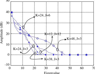
Eigenvalue K=24, J=6
K=12, J=12
K=48, J=3
K=38, J=3 K=24, J=3
The number of Clutter’s eigenvalues of the space-time covariance matrix is given by N e= K+J −1. For a given total KJ network’s dimensionality, the number of eigenvalues is obtained whenK =J[14]. In Figure 9, and for the same total space-time sample size ofKJ = 144, the plots are shown for a different ratios ofK/J and the same product ofK×J. We clearly show that forK =J = 12, the minimum number of eigenvalues is obtained, which points out the critical K/J array choice for the STAP problems.
6. CONCLUSION
In this paper, we have extended the effect of staggered PRF used by Klemm [13–15] and Reed [21, 22] with the optimum processor to the Reduced Rank processing with known covariance matrix. We applied the quadratic stagger pattern on two different RR methods, principal components and SINR metric presented from a direct form processor. The simulation results were presented to show the comparison between these two methods while using the Improvement Factor IF to exhibit the performance of the processor, using quadratic staggered PRF for eliminating the Doppler ambiguities and then improving the detection probability. It was also demonstrated that the RR approaches provide comparable performance as the optimum processing with reduced ranks.
Areas for future investigation include continued research into com-putationally efficient implementations, including parallel processing implementations, application to real STAP data sets, intelligent train-ing strategies, especially for 3D and circular STAP, and, for the signal-dependent methods, extensions and modifications with greater robust-ness to steering vector mismatches.
REFERENCES
1. Qu, Y., G. Liao, S.-Q. Zhu, X.-Y. Liu, and H. Jiang, “Performance analysis of beamforming for MIMO radar,”Progress In Electromagnetics Research, PIER 84 123–134, 2008.
2. Lee, K.-C., C.-W. Huang, and M.-C. Fang, “Radar target recognition by projected features of frequency-diversity RCS,”
Progress In Electromagnetics Research, PIER 81, 121–133, 2008. 3. Lee, K.-C., J.-S. Ou, and C.-W. Huang, “Angular-diversity radar
4. Wang, S., X. Guan, D. Wang, X. Ma, and Y. Su, “Fast calculation of wide-band responses of complex radar targets” Progress In Electromagnetics Research, PIER 68, 185–196, 2007.
5. Alyt, O. A. M., A. S. Omar, and A. Z. Elsherbeni, “Detection and localization of RF radar pulses in noise environments using wavelet packet transform and higher order statistics,”Progress In Electromagnetics Research, PIER 58, 301–317, 2006.
6. Haridim, M., H. Matzner, Y. Ben-Ezra, and J. Gavan, “Cooperative targets detection and tracking range maximization using multimode ladar/radar and transponders,” Progress In Electromagnetics Research, PIER 44, 217–229, 2004.
7. Gavan, J. and J. S. Ishay, “Hypothesis of natural radar tracking and communication direction finding systems affecting hornets flight,”Progress In Electromagnetics Research, PIER 34, 299–312, 2001.
8. Deng, H. and H. Ling, “Clutter reduction for synthetic aperture radar imagery based on adaptive wavelet packet transform,”
Progress In Electromagnetics Research, PIER 29, 1–23, 2000. 9. Weedon, W. H., W. C. Chew, and P. E. Mayes, “A step-frequency
radar imaging system for microwave nondestructive evaluation,”
Progress In Electromagnetics Research, PIER 28, 121–146, 2000. 10. Mooney, J. E., Z. Ding, and L. S. Riggs, “Performance analysis
of a glrt in late-time radar target detection,” Progress In Electromagnetics Research, PIER 24, 77–96, 1999.
11. Habib, M. A., B. Aissa, M. Barkat, and T. A. Denidni, “Ca-Cfar detection performance of radar targets embedded in “Non Centered Chi-2 Gamma” clutter,” Progress In Electromagnetics Research, PIER 88, 135–148, 2008.
12. Qu, Y., G. Liao, S.-Q. Zhu, and X.-Y. Liu, “Pattern synthesis of planar antenna array via convex optimization for airborne forward looking radar,”Progress In Electromagnetics Research, PIER 84, 1–10, 2008.
13. Klemm, R., “Comparison between monostatic and bistatic Antenna configurations for STAP,” IEEE Transactions on Aerospace and Electronic Systems, Vol. 36, No. 2, 596–608, 2000. 14. Klemm, R., “Space time adaptive processing, principles and
applications,” The Institution of Electrical Engineers, London, United Kingdom, 1998.
15. Klemm, R., “STAP with staggered PRF,” 5th International Conference on Radar Systems, Brest, May 17–21, 1999.
eigenanalysis methods,” IEEE Transactions on Aerospace and Electronic Systems, Vol. 32, No. 2, 532–542, 1996.
17. Ward, J., “Space-time adaptive processing for airborne radar,” Technical report 1015, Lincoln Laboratory, MIT, 1994.
18. Goldstein, J. S. and I. S. Reed, “Theory of partially adaptive radar,”IEEE Transactions on Aerospace and Electronic Systems, Vol. 33, No. 4, 1309–1325, 1997.
19. Haimovichand, A. M. and Y. B. Ness, “An eigenanalysis interference canceler,” IEEE Transactions on Signal Processing, Vol. 39, No. 1, 76–84, 1991.
20. Berger, S. D. and B. M. Welsh, “Selecting a reduced-rank transformation for STAP-A direct form approach,” IEEE Transactions on Aerospace and Electronic Systems, Vol. 35, No. 2, 722–729, 1999.
21. Gerci, J. R., J. S. Golstein, and I. S. Reed, “Optimal and adaptive reduced-rank STAP,” IEEE Transactions on Aerospace and Electronic Systems, Vol. 36, No. 2, 647–663, 2000.
22. Peckham, C. D., A. M. Haimovich, T. F. Ayoub, J. S. Goldstein, and I. S. Reed, “Reduced-rank STAP performance analysis,”