A Hybrid Method to Accelerate the Calculation of Two-Dimensional
Monostatic Radar Cross Section on PEC Targets
Chao Fei1, *, Xinlei Chen1, 2, Yang Zhang1, Zhuo Li1, 2, and Changqing Gu1
Abstract—This paper proposes a hybrid method to accelerate the calculation of the monostatic radar cross section (RCS) of perfect electric conducting (PEC) targets. In a sense, the proposed method can be considered as a fast adaptive cross approximation (FACA)-based method. The FACA is firstly used to compress the excitation matrix which comes from the beforehand defined incident plane waves. It decreases the time and memory on decomposing the excitation matrix compared with the conventional adaptive cross approximation (ACA). Furthermore, the computational complexity of iterative solution is reduced by using the sparsified ACA (SPACA) algorithm after dividing the target into blocks. Consequently, the proposed method is efficient for calculating two-dimensional (2D) monostatic RCS.
1. INTRODUCTION
The method of moment (MoM) is an accurate algorithm which has been used popularly to make the calculation of radar cross section (RCS). In a sense, the two-dimensional (2D) multi-angle monostatic RCS problems attract the attention for its importance of the military. For these problems, it is very time consuming for the conventional MoM as it needs to solve the matrix equation repeatedly. At the same time, the huge dense impedance matrix makes difficulties on each solution when the target is electrically large.
Fortunately, many fast methods have been proposed to accelerate the iterative solution of the MoM matrix equation. The adaptive cross approximation (ACA)-based algorithms [1–7] are relatively popular in recent years. For perfect electric conducting (PEC) targets within 50 wavelengths, the sparsified ACA (SPACA) algorithm [4, 5], which can be considered as a fast ACA (FACA)-based algorithm [7], is very efficient. Hence, it is used to accelerate the iterative solution in this paper.
However, the SPACA cannot reduce the number of iterative solutions of the matrix equation. For monostatic RCS problems, the excitation matrix, which comes from the incident plane waves, has low-rank property. Thus, in this paper, the FACA [7] is employed to compress the excitation matrix so as to reduce the number of iterative solutions of the matrix equation. Compared with the conventional ACA [1, 8], the FACA can save storage and give a more efficient sampling procedure for decomposing the excitation matrix when dealing with electrically large problems.
The remainder of this paper is organized as follows. In Section 2, the fundamental theory is introduced. In Section 3, the principles of the FACA and the SPACA are described in detail firstly, then the method using the FACA to accelerate the analysis of 2D monostatic RCS is introduced. In Section 4, examples and some discussion are presented so as to validate the efficiency and accuracy of the proposed method.
Received 28 June 2016, Accepted 26 August 2016, Scheduled 14 September 2016
* Corresponding author: Chao Fei ([email protected]).
1 Key Laboratory of Radar Imaging and Microwave Photonics, Ministry of Education, College of Electronic and Information
2. ELECTROMAGNETIC THEORY
To analyze the electromagnetic (EM) scattering problem of an arbitrary shaped perfect electric conducting (PEC) target, the Rao-Wilton-Glisson (RWG) [9] basis function and the surface integral equation (SIE) are used to expand the induced surface current and describe the relationship between the divided triangle elements.
An element of the electric field integral equation (EFIE) is expressed as
ZmnE =jkη
Tm±
Tn±
Gr,r fm(r)·fnr− 1
k2∇ ·fm(r)∇·fn
rdsds, (1)
where fm(r) is the mth RWG basis function which is considered as the field point, fn(r) the nth RWG basis function which is considered as the source point, ∇· (∇·) the divergence operator on the field (source) point, k the wave number, η the intrinsic impedance of the free space, and
G(r,r) =e−jk|r−r|/(4π|r−r|) the Green’s function in free space.
An element of the magnetic field integral equation (MFIE) is expressed as
ZmnM = 1 2
T± m
fm(r)·fnrds−
T± m
(fm(r)×nˆm)·
P.V.
T± n
∇Gr,r×fnrds
ds, (2)
where∇is the gradient of a scalar and ˆnm the unit direction vector of themth basis function.
The element of the general impedance matrix in the combined field integral equation (CFIE) is calculated as
Zmn=αZmnE + (1−α)ηZmnM , (3)
and α= 0.5 here.
If there are M plane waves which come from different incident angles irradiate the target for a monostatic RCS problem, the dimension of excitation matrix V is N ×M. Here, N is the number of RWG basis functions.
Finally, the MoM matrix equation is presented as
ZI=V, (4)
where Z∈CN×N is a dense impedance matrix, and I∈CN×M is the solution matrix which is needed to calculate the RCS. From Eq. (4), it can be seen that the impedance matrix equation should be solved
M times for the monostatic RCS calculation.
3. ACCELERATED SOLUTION VIA FACA-BASED METHOD
3.1. Principle of FACA
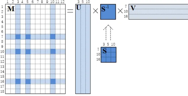
The FACA [7] is a low-rank decomposition method based on the fast adaptive cross sampling (FACS) [5], which can efficiently find the important columns and rows of a rank-deficient matrix. Thus, the FACA can provide a more efficient compression of an impedance submatrix between two well-separated blocks in the MoM than the conventional ACA [1]. Here, the compression of a low-rank matrixM∈Cm×nis set to be an example to describe the FACA as follows.
The FACA is an iterative method. Firstly,sn columns andsn rows are uniformly sampled fromM
with the sampling number
sn= 2n·s0. (5)
for the nth iteration. Here,sn is the sampling number of the nth iteration ands0 the initial sampling value, which is assigned artificially.
Secondly, the elements belong to both the sampled columns and rows which make up a new matrix
Mn (for thenth iteration), and the ACA is used on it.
Mn≈UnVn (6)
is the decomposed form acquired by the ACA.Un∈Csn×kn,Vn∈Ckn×sn, andkn is the effective rank
Thirdly, the convergence criterion [5]
|kn−kn−1| ≤β|sn−sn−1| (7)
is judged, where the constant β is set to [0.01,0.1] usually. If Eq. (7) is met, the iteration terminates. When the criterion is met, the serial numbers of the sampled columns and rows are saved. With them, according to the matrix decomposition algorithm (MDA) [10], Mcan be decomposed into
M≈US−1V, (8)
where U ∈ Cm×k, V ∈ Ck×n, and S−1 ∈ Ck×k are the decomposed matrices of the FACA as the schematic diagram Fig. 1. The parameter k is the final sampling number of the FACA, and it is assumed that k= 3 in Fig. 1. U-matrix comes from the sampled columns. V-matrix comes from the sampled rows. S-matrix consists of the elements which belong to both the sampled columns and rows, and S−1 is the inverse matrix.
Figure 1. The schematic diagram of the FACA withk= 3.
3.2. Compression of Impedance Matrix
The SPACA [4, 5] can be viewed as an improved FACA [7]. It is used in this paper to compress the impedance matrix of the MoM.
After dividing the target into blocks with the octal tree structure, the near-block pairs and far-block pairs are classified by the position relationship. Two far-blocks, which are overlapping or adjacent, are considered as a near-blocks pair; otherwise, they are a far-block pair. At each level, impedance matrices of far-block pairs are compressed by the SPACA. For example, Zi,j, the impedance matrix between theith block and thejth block, is compressed with the following process.
Firstly,Zi,j is decomposed by the FACA as
Zi,j ≈ZiZ−s1ZTj, (9)
whereZi(Zj)∈Ca×s comes from the interaction between all basis functions in theith (jth) block and the sampled basis functions in the jth (ith) block. The parameter a is the average number of basis functions of all blocks, and the parameters is the sampling number of the FACA.
Then, the ACA-singular value decomposition (ACA-SVD) [2] and the QR decomposition are used to further compressZi,j as [5]
Zi,j ≈AiQˆiSRQˆTjATj, (10)
3.3. Compression of Voltage Matrix
The SPACA can accelerate the iterative solution of the impedance matrix equation for each excitation. However, it cannot reduce the number of excitations for the monostatic RCS. In this paper, the FACA [5, 7] is employed to reduce the number of excitations because the voltage matrix has low-rank property for monostatic RCS problems. For the right-hand side, the voltage matrixV∈CN×M can be decomposed by the FACA [7] as
V≈PD−1Q, (11)
whereP∈CN×q,Q∈Cq×M and D∈Cq×q. q is the sampling number of the FACA. Substituting Eq. (11) into Eq. (4), we have
ZI≈PD−1Q. (12)
Thus,
I≈(Z−1P)D−1Q=JD−1Q. (13)
In Eq. (13), the following equation needs to be iteratively solved
ZJ=P. (14)
From Eq. (14), it can be seen that the impedance matrix equation only needs to be solved q times, where q is the effective rank of V and typically much smaller than M. Thus, the computation time of the monostatic RCS is remarkably reduced with the help of the FACA.
The conventional ACA [1] has been used to speed up the monostatic RCS calculation in [2], in which the excitation matrix is compressed as
V≈UvVv, (15)
whereUv ∈CN×qand Vv∈Cq×M are the ACA decomposed matrices of V. Here, we assume that the effective ranks evaluated by the FACA and ACA are the same. Similarly, if substituting Eq. (15) into Eq. (4), the ACA can also cut down the number of iterative solutions of matrix equation.
The disadvantage of the ACA is that bothUv and Vv have to be stored. However, in the FACA, only Pand D−1 need to be stored, and the memory of Q can be saved. We can calculate each column of Q when it is needed in the RCS calculation process. The computational complexity of the ACA is
O(q2(N +M)) [1]. However, the computational complexity of the FACA is O(q3)+O(q(N +M)) [7], whereO(q3) is the complexity of the FACS andO(q(N+M)) the complexity of generatingPandQ(the LU decomposition of D has been calculated in the FACS process [5]). Thus, another advantage of the FACA is that it can save the decomposition time of the voltage matrix compared with the conventional ACA.
4. EXAMPLES AND DISCUSSION
As the efficiency of the SPACA accelerating iterative solution has been validated [4, 5], this section is only to show the accuracy and efficiency of the FACA when dealing with 2D monostatic RCS problems. For the following examples, all impedance matrices are compressed by the SPACA. Analysis and discussion are presented as follows.
4.1. Cube
Without loss of generality, the monostatic RCSs of several cube models are discussed firstly. Sidelength
a of the cubes is a variable, and the efficiency is shown with the increase of a. Models are irradiated by 300 MHz plane waves which are defined at θ∈[0◦,180◦] and ϕ∈[0◦,360◦) both with step 2◦, where the number of incident waves is 16380 and the polarization ˆθ. The ACA threshold is set to 10−4 and
β = 0.01. The accuracy error of the compressed decomposition of V is calculated by
error= Vsamp−VF
whereV is the original voltage matrix andVsampthe decomposition form just as Eq. (11) and Eq. (15).
· F is the Frobenius-norm.
For these models, the sampling number, time and memory on compressingV are listed in Table 1. We can see that the two methods have similar sampling number and decomposition error. However, the FACA provides a more efficient decomposition procedure than the conventional ACA. With the increase of the number of basis functions, the time-reduction and memory-saving are more and more remarkable.
Table 1. Sampling comparison of the models.
Sampling number Time (s) Memory (MB) Error
a(m) Unknowns ACA FACA ACA FACA ACA FACA ACA FACA 2 8118 367 370 6.07 7.77 67.8 24.0 2.03×10⁻⁴ 2.01×10⁻⁴ 2.5 12690 491 481 11.97 12.11 108.9 48.4 2.05×10⁻⁴ 2.32×10⁻⁴ 3 18342 614 611 18.73 17.09 162.8 88.5 2.25×10⁻⁴ 2.55×10⁻⁴ 3.5 25656 757 740 32.01 24.37 243.0 96.66 2.81×10⁻⁴ 3.46×10⁻⁴
4.2. Rocket
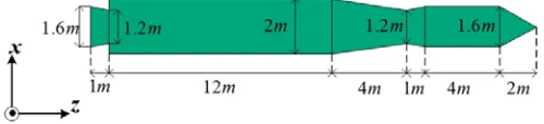
Then, a more complex target, a 16λrocket model, as shown in Fig. 2 is analyzed. Incident plane waves are defined atθ∈[0◦,180◦],ϕ∈[0◦,360◦) both with the step 1◦and the total numberM = 65160. The plane wave is at 200 MHz with the polarization ˆθ. The numerical model exhibitsN = 44088 unknowns.
Figure 2. The rocket model.
Table 2. Computation comparison on the rocket model.
ACA FACA Sampling number 819 810 Time of compressingV(s) 96.5 47.7 Storage of compressedV(MB) 682.6 277.5
Table 2 gives the comparison of the FACA and ACA on compressing V (the ACA threshold is 10−4, β = 0.01 and s0 = 40). It can be seen that the FACA provides a faster decomposition and requires less memory. The number of iterative solutions of the impedance matrix equation is reduced from 65160 to 810 by the FACA. It means that the iterative solution time is cut down by a factor of 80. The solution times are also cut even compared to using the ACA. Because the rocket is a rotational symmetric model, only the monostatic RCSs atϕ= 0◦ are shown in Fig. 3. Obviously, the RCS curves have a good match. The relative errors of several ϕvalues are presented in Fig. 4. As we can see, the curves show that the relative errors are mostly below−10 dB. Here, relative error is calculated as
relative error= 10 log10RCSACA−RCSF ACA
RCSACA
, (17)
Figure 3. Monostatic RCS of the rocket model at 200 MHz (ϕ= 0◦).
Figure 4. Relative error of the rocket model at 200 MHz.
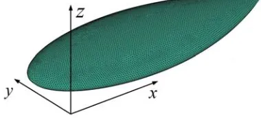
4.3. Almond
Finally, a 252.3744 mm almond (Fig. 5) at 15 GHz is analyzed. The incident plane waves are defined at the same angles and polarization as the example II. It has 36225 unknowns, and the comparison is listed in Table 3.
Figure 5. The almond model
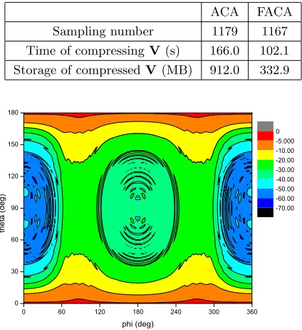
In this example, the ACA threshold is 10−5,β = 0.01 ands
Table 3. Computation comparison on the almond model.
ACA FACA Sampling number 1179 1167
Time of compressingV(s) 166.0 102.1 Storage of compressedV(MB) 912.0 332.9
Figure 6. Monostatic RCS of the PEC almond at 15 GHz. (Unit: dBsm)
Figure 7. Relative error of the PEC almond at 15 GHz. (Unit: dB)
Fig. 7. After the FACA compression, only 1167 excitation vectors need to be solved. Thus, the FACA can speed up the calculation of the monostatic RCS than the conventional SPACA in which the number of the right hand vectors is 65160.
5. CONCLUSION
ACKNOWLEDGMENT
This work was supported by Funding of Jiangsu Innovation Program for Graguate Education and the Fundamental Research Funds for the Central Universities under Grant No. kfjj20160406, the National Natural Science Foundation of China under Grant No. 61501227 and 61071019, the Postdoctoral Science Foundation of China under Grant No. 2015M581789, the Fundamental Research Funds for the Central Universities under Grant No. NJ20160011, and the Foundation of State Key Laboratory of Millimeter Waves, Southeast University, China, under Grant No. K201719.
REFERENCES
1. Zhao, K., M. N. Vouvalis, and J. Lee, “The adaptive cross approximation algorithm for accelerated method of moments computations of EMC problems,”IEEE Trans. Electromagnetic Compatibility, Vol. 13, No. 4, 763–772, Nov. 2005.
2. Heldring, A., J. M. Rius, J. M. Tanayo, J. Parron, and E. Ubeda, “Multiscale compressed block decomposition for fast direct solution of method of moments linear system,”IEEE Trans. Antennas and Propag., Vol. 59, No. 2, 526–536, Feb. 2011.
3. Tanayo, J. M., A. Heldring, and J. M. Rius, “Multilevel adaptive cross approximation (MLACA),” IEEE Trans. Antennas and Propag., Vol. 59, No. 12, 4600–4608, Dec. 2011.
4. Heldring, A., J. M. Tanayo, C. Simon, E. Ubeda, and J. M. Rius, “Sparsified adaptive cross approximation algorithm for accelerated method of moments computations,” IEEE Trans. Antennas and Propag., Vol. 61, No. 1, 526–536, Jan. 2013.
5. Chen, X., C. Gu, Z. Niu, and Z. Li, “Fast adaptive cross-sampling scheme for the sparsified adaptive cross approximation,”IEEE Antennas and Wireless Propagation Letters, Vol. 13, 1061–1064, 2014. 6. Chen, X., C. Gu, Z. Li, and Z. Niu, “Sparsified multilevel adaptive cross approximation,” IEEE
Asia-Pacific Conference on Antennas and Propagation, 971–973. 2014.
7. Chen, X., C. Gu, J. Ding, Z. Li, and Z. Niu, “Multilevel fast adaptive cross-approximation algorithm with characteristic basis functions,”IEEE Trans. Antennas and Propag., Vol. 63, No. 9, 3994–4002, Sep. 2015.
8. Schroder, A., H. D. Bruns, and C. Schuster, “A hybrid approach for rapid computation of two-dimensional monostatic radar cross section problems with the multilevel algorithm,” IEEE Trans. Antennas and Propag., Vol. 60, No. 12, Dec. 2012.
9. Rao, S. M., D. R. Wilton, and A. W. Glisson, “Electromagnetic scattering by surfaces of arbitrary shape,” IEEE Trans. Antennas and Propag., Vol. 30, No. 2, 409–418, May 1982.