The Use of Point Pattern Analysis in Archaeology: Some Methods and Applications

(1)

Scholarship@Western

Electronic Thesis and Dissertation Repository

8-27-2015 12:00 AM

The Use of Point Pattern Analysis in Archaeology: Some Methods

and Applications

James R. Keron

University of Western Ontario Supervisor

Dr C.J. Ellis

The University of Western Ontario Joint Supervisor Dr E. Molto

The University of Western Ontario Graduate Program in Anthropology

A thesis submitted in partial fulfillment of the requirements for the degree in Doctor of Philosophy

Follow this and additional works at: https://ir.lib.uwo.ca/etd Part of the Anthropology Commons

Recommended Citation Recommended Citation

Keron, James R., "The Use of Point Pattern Analysis in Archaeology: Some Methods and Applications" (2015). Electronic Thesis and Dissertation Repository. 3137.

https://ir.lib.uwo.ca/etd/3137

This Dissertation/Thesis is brought to you for free and open access by Scholarship@Western. It has been accepted for inclusion in Electronic Thesis and Dissertation Repository by an authorized administrator of

(2)

(Thesis format: Monograph)

by

James R. Keron

Graduate Program in ANTROPOLOGY

A thesis submitted in partial fulfillment of the requirements for the degree of

Doctor of Philosophy

The School of Graduate and Postdoctoral Studies The University of Western Ontario

London, Ontario, Canada

(3)

ii

Abstract

This study explores a field of spatial statistics known as Point Pattern Analysis (PPA)

and its application in archaeology. The overall goal is to provide a resource which will guide

and assist the reader in the proper application of PPA. Past archaeological applications are

combined with more recent geographical and statistical mathematics to create a more

inter-disciplinary, synthesized approach. Included are a discussion of analytical methods and two

detailed case studies/applications.

The study begins with an overview of PPA approaches in archaeology, starting with a

general introduction and several commonly understood concepts such as first and second

order effects and simple and labeled point patterns. It also describes options for calculating

statistical significance and their appropriate uses which depend on the analysis being

performed --something which is not well articulated in the literature. It goes on to describe

appropriate techniques for analysis introducing another new concept called resolution focus,

which facilitates comparison of various statistics in the analysis of first order effects. Finally,

it provides logical structured approaches to conducting a PPA and selecting appropriate

statistics for various kinds of analysis including some refined and new routines. A series of

PPA statistics developed in R are provided.

The first case study analyzes the distribution of surface material in the 1.9 ha

Davidson Archaic site in Ontario. An analysis of first and second order effects of the

distribution of lithic debitage using multiple statistics leads to the conclusion that the Broad

Point occupation represents an aggregation site with a series of similar clusters representing

socially distinct groups of people. A second order analysis of the distribution of more formal

artifacts shows a more complex deposition than the flake clusters.

The second case study examines the distribution of discrete genetic traits in the

Kellis-2 cemetery in Egypt evaluating the hypothesis that the cemetery was organized on a

kinship basis and that male kin ties governed grave placement. In addition, it is shown that a

lower than expected number of males in the cemetery is not spatially random but tends to

(4)

iii

Keywords

Spatial statistics, point pattern analysis, bioarchaeology, unconstrained clustering, discrete

(5)

iv

Acknowledgments

First I need to thank to my supervisor, Dr Chris Ellis, for guiding me through the entire

process. He read and commented on many drafts of comps, conference papers, and the final

dissertation always returning comments promptly. I am also grateful for the opportunity of

participating in the Davidson site work over the last seven years in both the full time summer

excavations and other occasional work at the site. I should also mention his generous

provision in allowing me to participate in the analysis for various publications over the last

few years.

Secondly, I would like to thank my co-supervisor, Dr. El Molto for is work helping me

through the analysis of the Kellis-2 material. In fact I think the first discussion on the back of

a napkin in the grad club happened before I actually started the program at a chance

encounter back in 2008. His encouragement of my interest in statistics in general and spatial

stats in particular over the past few years has been enlightening and useful. Finally the data

from Kellis-2 provided an opportunity to push the analysis of spatial data beyond anything I

would have imagined. Indeed it could be taken further by integrating genetics into the

analysis.

Next I would like to thank the PhD examination board, Dr. James Conolly, Dr. Jacek

Malczewski, Dr. Jean-Francois Millaire, and Dr. Andrew Nelson for the time they spent

reading this and all of the helpful comments (and penetrating questions) at the defence. Their

comments improved the overall dissertation and will provide a great first step in revisions on

the road to publication.

After that there is a long list of people who intentionally or otherwise have influenced my

walk down this road. Dr. Jean-Francois Millaire provided insight and guidance in the

intricacies of GIS. Dr. Micha Pazner and Dr. Jacek Malczewski steered me into the field of

point pattern analysis. Dr. Mike Spence pointed out the very useful framework of

Stojanowski and Schillaci (2009). Dr. Mike Bauer in Computer Science steered me into the

use of R as well as other opportunities that were not pursued in this research. Ed Eastaugh

and Dr. Lisa Hodgetts graciously allowed the inclusion of some unpublished magnetic

(6)

v

University who responded quickly to a number of inquiries of mine related to both his

software package, TFQA, as well as related statistical questions. This help was invaluable.

I should also mention two other grad students, Matt Teeter and Tiffany Sarfo who were also

working on Kellis-2 material. Conversations with Matt helped generalize some of this and

Tiffany graciously volunteered to alpha test the newly developed R statistical routines on her

data.

Of course there are the other members of Chris Ellis’ retired mafia, Darryl Dann and Larry

Neilson whose dedicated lab work had all of the material washed cataloged and ready for

analysis.

I would also like to thank Dr. Dan Jorgensen for his cogent comments on the issue of kinship

and post marital residence towards the Kellis case study and also, while not directly related to

this dissertation, for giving me the opportunity to teach an introductory statistics course. It

was an extremely rewarding activity and, while I grumbled that I had not worked so many

hours for so little pay since I worked on a dairy farm as a teenager, I would not have missed

it for the world.

Finally, I would like to thank my family members Brian, Rob, and Tara for their support and

I cannot forget my fellow grad student, daughter Catherine. Also I should mention my

mother who, while she did not live to see the completion, was very encouraging of my

endeavors. Finally, my wife, Jan Vicars, for much encouragement and patience me as I

worked through the requirements of the degree and lest I forget the ordeal of proof reading a

final draft of this dissertation as well as my comprehensives. Any errors retained are solely

(7)

vi

List of Tables

Table 2-1: Nearest Neighbour Between Types – CSR - TFQA... 29

Table 2-2: Nearest Neighbour Between Types Random Labeling ... 29

Table 2-3: Area Data Statistics ... 36

Table 2-4: Point Pattern Statistics ... 37

Table 4-1: Surface Artifacts by Type... 78

Table 4-2: A- Statistic on Non Chert Flakes ... 82

Table 4-3: Flake Typology... 94

Table 4-4: Flake Types by Spatial Cluster ... 99

Table 4-5: A-statistic Coarse Flakes by Type ... 100

Table 4-6: Counts of Flakes by Activity Cluster ... 105

Table 4-7: Percentages of Flakes by Activity Cluster ... 105

Table 4-8: Proximity Count ... 120

Table 4-9: Count of Broad Point Artifacts - Inside and Outside RMS Circles... 125

Table 4-10: Broad Point Artifacts - Nearest Neighbour ... 127

Table 4-11: Non Diagnostic Tools ... 130

Table 4-12: A-statistic Non Diagnostic Tool Forms... 132

Table 5-1: Proximity Count - Males and Females ... 158

Table 5-2: Local Density Analysis Males and Females... 160

(12)

xi

Table 5-5: Summary of Individual Trait Analysis ... 166

Table 5-6: Cartico-clinoid Bridge - Cross Nearest Neighbour by Sex ... 169

Table 5-7: Cartico-clinoid Bridge - Cross Proximity Count by Sex ... 170

Table 5-8: Clino-clinoid Bridge Cross Nearest Neighbour by Sex ... 171

Table 5-9: Clino-clinoid Bridge Cross Proximity Count by Sex ... 171

Table 5-10: Divided Jugular Canal - Cross Nearest Neighbour by Sex ... 172

Table 5-11: Divided Jugular Canal Cross Proximity Count by Sex ... 172

Table 5-12: Infraorbital Suture Cross Nearest Neighbour by Sex ... 173

Table 5-13: Infraorbital Suture Cross Proximity Count by Sex ... 173

Table 5-14: Intermediate Condylar Canal Cross Nearest Neighbour by Sex ... 174

Table 5-15: Intermediate Condylar Canal Cross Proximity Count by Sex ... 174

Table 5-16: Open Foramen Spinosum Cross Nearest Neighbour by Sex ... 175

Table 5-17: Open Foramen Spinosum Cross Proximity Count by Sex ... 175

Table 5-18: Ossified Apical Ligament Cross Nearest Neighbour by Sex ... 176

Table 5-19: Ossified Apical Ligament Cross Proximity Count by Sex ... 176

Table 5-20: Parietal Foramen Cross Nearest Neighbour by Sex ... 177

Table 5-21: Parietal Foramen Cross Proximity Count by Sex ... 177

Table 5-22: Pharyngeal Fossa Cross Nearest Neaighbour by Sex ... 178

(13)

xii

Table 5-25: Post Condylar Canal Absent Cross Proximity Count by Sex ... 179

Table 5-26: Pterygobasal Spur Cross Nearest Neighbour by Sex ... 180

Table 5-27: Pterygobasal Spur Cross Proximity Count by Sex ... 180

Table 5-28: Supraorbital Foramen Cross Nearest Neighbour by Sex... 181

Table 5-29: Supraorbital Foramen Cross Proximity Count by Sex ... 181

Table 5-30: Zygomatico-facial Foramen Absent Cross Nearest Neighbour by Sex ... 182

Table 5-31: Zygomatico-facial Foramen Absent Cross Proximity Count by Sex ... 182

Table 5-32: Asterionic Ossicle Cross Nearest Neighbour by Sex ... 183

Table 5-33: Asterionic Ossicle Cross Proximity Count by Sex ... 183

Table 5-34: Lamdic Ossicle Cross Nearest Neighbour by Sex ... 184

Table 5-35: Lambdic Ossicle Cross Proximity Count by Sex ... 184

Table 5-36: Lambdoidal Ossicle Cross Nearest Neighbour by Sex ... 185

Table 5-37: Lambdoidal Ossicle Cross Proximity Count by Sex ... 185

Table 5-38: 15 Traits Used for Second Run ... 190

Table 5-39: Traits Used for the Third Run ... 191

(14)

xiii

List of Figures

Figure 1-1: Fluted Point Fragments in Feature 1, Crowfield Site... 5

Figure 2-1: KD Radius at 50 m ... 31

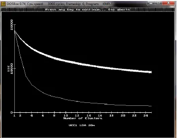
Figure 3-1: SSE Plot from Unconstrained Clustering... 50

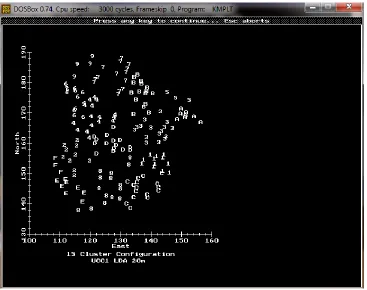
Figure 3-2: TFQA Plot of Unconstrained Clustering ... 51

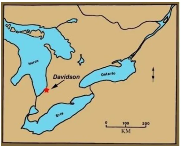
Figure 4-1: The Davidson Site in Southern Ontario ... 55

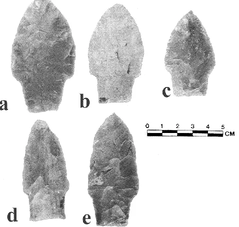
Figure 4-2: Genesee Points on Onondaga from Davidson... 55

Figure 4-3: Genesee-like Points on Subgreywacke from Davidson ... 56

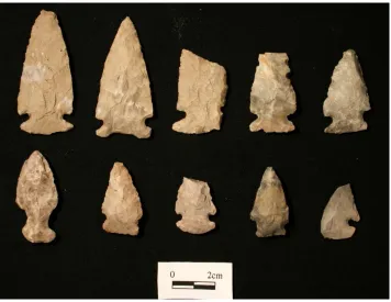
Figure 4-4: Adder Orchard Points from the Adder Orchard Site ... 56

Figure 4-5: Smallpoints from Davidson ... 57

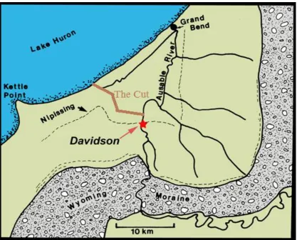
Figure 4-6: The Davidson Site Local Topography ... 58

Figure 4-7: Davidson Site Extent - Current Air Photo ... 60

Figure 4-8: Davidson Site Extent - 1978 Air Photo ... 61

Figure 4-9: Kenyon's Map on 1978 Air Photo ... 62

Figure 4-10: 2006 Test Pits Relative to Kenyon's Work ... 64

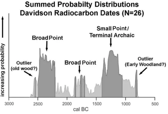
Figure 4-11: Calibrated C14 Dates Jan 2015 – Dark One Sigma, Light Two Sigma ... 65

Figure 4-12: Davidson Surface Collection by Time Period ... 67

(15)

xiv

Figure 4-15: Davidson Site Main Excavations ... 74

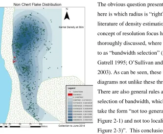
Figure 4-16: Distribution of Non Chert Flakes ... 83

Figure 4-17: Distribution of Coarse Flakes ... 85

Figure 4-18: Coarse Flakes - Medium Resolution Focus ... 88

Figure 4-19: Coarse Flakes – Fine Resolution Focus ... 90

Figure 4-20: Coarse Flakes – Getis-Ord Gi* on 5 m Fishnet ... 92

Figure 4-21: Coarse Flakes - Getis-Ord Gi* on 3 m Fishnet ... 93

Figure 4-22: Coarse Flakes by Type ... 97

Figure 4-23: Coarse Flakes by Spatial Cluster ... 98

Figure 4-24: SSE Plot LDEN = 5 m ... 103

Figure 4-25: Unconstrained Clustering of Coarse Flake Types... 104

Figure 4-26: Activity Clusters 7, 8 and 9 ... 106

Figure 4-27: Activity Clusters 1 and 2 ... 108

Figure 4-28: Activity Clusters 3,4 and 5 ... 110

Figure 4-29: Activity Clusters 6 and 10 ... 111

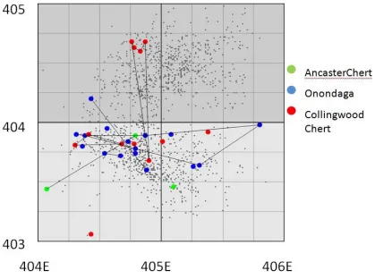
Figure 4-30: Distribution of Small Point and Broad Point Artifacts ... 114

Figure 4-31: Small Point Artifacts and the Magnetometer Data ... 116

Figure 4-32: Small Point Artifact and Magnetometer Data - North End ... 117

(16)

xv

Figure 4-35: Broadpoint Artifact Kernel Density ... 124

Figure 4-36: Broad Point Artifacts by Raw Material... 126

Figure 4-37: Broad Point Artifacts by Type ... 128

Figure 4-38: Broad Point Artifacts by Description ... 129

Figure 4-39: Non Diagnostic Tool Forms ... 133

Figure 4-40: Comparison of Spatial Cluster Structure ... 136

Figure 4-41: The Old hedge Row / Fence Line ... 138

Figure 5-1: Location of the Dakhleh Oasis ... 146

Figure 5-2: The Full Extent of K2 ... 147

Figure 5-3: Excavated Portion of K2 ... 148

Figure 5-4: Males and Females - Large Sample ... 159

Figure 5-5: Male Female Distribution - Smaller Sample... 164

Figure 5-6: %SSE Values from All Individuals and 29 Traits ... 189

Figure 5-7: Confidence Envelopes for All Traits and All Individuals... 192

Figure 5-8: %SSE by Cluster for the Best Radius from Each Run ... 193

Figure 5-9: Close Up of Figure 5-8 with the Higher Cluster Numbers ... 194

Figure 5-10: Cluster Assignments for 14 Traits and All Individuals... 196

Figure 5-11: Clusters with Excessive Missing Males ... 200

(17)

xvi

Figure B-3 Carotico-clinoid Bridge………...229

Figure B-4 Clino-clinoid Bridge………...230

Figure B-5 Divided Hypoglossal Canal………...231

Figure B-6 Divided Jugular Canal………...232

Figure B-7 Frontal Grooves………...233

Figure B-8 Frontal-Temporal Articulation………...234

Figure B-9 Infraorbital Suture………...235

Figure B-10 Intermediate Condylar Canal ………...236

Figure B-11 Marginal Foramen………...237

Figure B-12 Mendosal Suture ………...238

Figure B-13 Metopic Suture ………...239

Figure B-14 Mylohyoid Bridge………...240

Figure B-15 Notochord Remnant………...241

Figure B-16 Open Foramen Spinosum………...242

Figure B-17 Os Japonicum ………...243

Figure B-18 Ossified Apical Ligament………...244

Figure B-19 Parietal Foramen………...245

Figure B-20 Pharyngeal Fossa ………...246

(18)

xvii

Figure B-23 Pterygobasal Spur………...249

Figure B-24 Pterygospinous Spur………...250

Figure B-25 Supraorbital Foramen………...251

Figure B-26 Trochlear Spur ………...252

Figure B-27 Tympanic Dehiscence………...253

Figure B-28 Zygomatico-facial Foramen Absent………...254

Figure B-29 Asterionic Ossicle………...255

Figure B-30 Bregmatic Ossicle………...256

Figure B-31 Coronal Ossicle………..………...257

Figure B-32 Lambdic Ossicle………...258

Figure B-33 Lambdoidal Ossicle………...259

Figure B-34 Occipito-mastoid Ossicle ………...260

Figure B-35 Parietal Notch Ossicle ………...261

Figure B-36 Pterionic Ossicle ………...262

Figure B-37 Sagittal Ossicle………...263

(19)

xviii

List of Appendices

Appendix A: Glossary of Terms ... 225

Appendix B: Kellis Figures ... 227

(20)

Chapter 1

1 Introduction and Background

1.1 Background

All human behaviour, past and present, occurs in a real time spatial context. In reality,

most of our behaviours cannot be traced in terms of material data. This is a real challenge

for archaeology since its defining role is the reconstruction of past human behaviours.

The reconstruction of past spatial environments offers a potential means of addressing the

reconstruction of a portion of past human behaviour. It is the purpose of this study to

examine the distribution of archaeological material utilizing spatial statistics.

Specifically, I use an analytical technique called Point Pattern Analysis (PPA) (Bailey

and Gatrell 1995). The specific goals of this study are to develop new, and refine

existing, spatial statistical methods and to demonstrate their utility through their

application to two archaeological data sets; a) the artifactual data recovered through

surface collections from the Davidson Late Archaic site in Ontario (ca. 2500-800 BC);

and b) the biological/skeletal data recovered from the Kellis-2 Christian cemetery in

Egypt (ca. 100- 400 AD). Since, as noted, all archaeological material has a spatial

context, in my opinion, there is a great deal of information to be obtained through the

analysis of spatial distributions of various artifacts and other data sets. The same is

certainly true for the distributions of archaeological sites across the landscape but, for

purposes here, I will concentrate on the distribution of artifacts/biological traits within a

single site context.

Archaeologists have had a controversial relationship with statistics over time. During

1960/70s with the advent of the “New Archaeology” statistical applications were in

vogue, such that American Antiquity looked more like the Journal of the Royal Statistical

Society with many pages of mathematical notation. The post-processual movement in the

1980s reversed this trend, as statistics, and indeed, the scientific method, became passé,

(21)

theory in archaeology within a growing trend that Trigger (2006) calls “pragmatic

synthesis”. This synthesis included spatial analyses.

The term “spatial” is used to distinguish this type of statistical analysis from classical

statistics. The first question emerging is what are “spatial statistics” and how do they

differ from the classical statistics that were conventionally taught in postsecondary

education? Basically, spatial statistics involves the application of specific techniques

using the actual location in geographic space to make inferences about various

phenomena. As a hypothetical example, a confidence interval that states that 34% +/-

2.5%, 19 times out of 20, of Canadians would vote NDP if an election were called today

takes no notice of the location of various voters. Each voter is located in a single riding,

but the actual location of the voter is ignored. Indeed, to be accurate, the sample must be

randomly selected from the set of all Canadian voters. The polling industry may give

regional breakdowns, and sometimes will be separated by provinces, but this separation

does not qualify this analysis as spatial statistics. In order to be a spatial statistic, the

mathematical calculation of the statistic needs to make use of the exact spatial location of

each variate, for example, in archaeology, exact coordinates for each artifact relative to a

datum point as plotted in a controlled surface pickup (CSP).

A fundamental difference between spatial and classical statistics is that the latter assumes

that data are independent of each other. For example, in sampling, any data item is as

equally likely to occur as another. In fact, lack of independence effectively negates or at

least complicates the application of classical statistical methods. When it comes to

application of statistical methods to human activity in space, the least likely thing that we

could expect to find is to have the events randomly distributed in space, a condition

called Complete Spatial Randomness (CSR). In geography, a concept called Tobler’s

First Law of Geography (Tobler 1970) states that all things are related in geographic

space and nearby things are more related than distant things, in effect, the closer the

geographical proximity, the more similar the data. An example of this is elevation points

on a landscape where, barring the occasional precipice, your next step is very likely to be

approximately the same elevation as your previous one. In human activity, nearby sites

(22)

occurring with more distant sites. In spatial statistics this factor is known as spatial

autocorrelation and it almost always occurs in human activity. Fortunately, spatial

autocorrelation does not negate the application of spatial statistics as it would have in

classical statistics. It is the nature of these relationships in space that has the most

potential for better understanding past human activity. Interestingly, the recognition of

this problem within anthropology started when Francis Galton critiqued a paper by E.B

Tylor in 1889 --his critique has subsequently been recognized as statistical in nature and

become known as Galton’s Problem (Stocking 1968; Naroll 1961, 1965).

Spatial data has two primary components. Like data in classical statistics, it has one or

more values or attributes which describe the nature of the specific phenomena for each

data element being considered. For example, this characteristic could be the projectile

point type, the raw material, measurements of the artifact, etc. In addition, the second

type of component defines the location of this data element in geographical space. This

spatial component of data can be represented in three ways: a point, a line or an area

object. A point has the Cartesian coordinates (x,y) of each particular item of interest, such

as the east and north components of a position coordinate of a number of sites or artifact

finds on the landscape. A line is exemplified by a road on a map but this form of spatial

data is not used in this study. An area unit is a subsection of a site or region and can be

any shape. For example, it could be as small as a 50cm square or as large as a Borden

unit, county or province. The key difference is that with the point data each instance has

its own specific (x,y) coordinates, whereas an area unit can be defined with many

different shapes, although each unit describes a unique, non-overlapping block of space.

Of course, it is possible to convert from one to the other especially from point to area

data, but the reverse is problematic and should generally be avoided. Point data could be

summarized into an area unit by counting the number of instances of a point pattern

within a unit (e.g. the number of flakes in a five metre square). Problems with this

conversion are described in more detail below. It is important to emphasize that each of

these classes of data have their own set of appropriate statistical techniques, including

(23)

Further, in selecting a specific technique, it is necessary to consider the nature of the data

to be analyzed (e.g. nominal, ordinal, interval, and ratio). For example, one set of data might

have the size of each site in hectares and a second set of data might have the particular site

type: the first is ratio data and the second is clearly nominal. As with classical statistics, some

statistical processes are appropriate for nominal data and some are appropriate for ratio data.

For example, applying a technique called Moran’s I to nominal data such as a set of

locations encoded with 0 meaning absent and 1 meaning present is invalid, though results can

be obtained. These specific data types (nominal/ratio) apply to both of our two main classes

of data (point or area unit).

In this study I will concentrate primarily on point pattern data as such data is very common in

archaeology. Obviously analytical techniques for both types are important but, for our

purposes, the main focus will be on point pattern analysis since, in my opinion, point pattern

analysis of archaeological materials in the past has been weak. It should be noted that

archaeological data and geographical data are often different. Geographers often deal with

data that are summarized by areal unit whereas archaeologists deal more often with point

pattern data; hence the emphasis herein. However, both fields have to be cognizant of the

strengths and weaknesses of the statistical methods. In this regard Bailey and Gatrell (1995) and/or O’Sullivan and Unwin (2003) provide excellent discussions of the application of

spatial statistics.

To further illustrate questions that arise within point pattern data, consider Feature 1 at the

Crowfield site in southwestern Ontario (Deller et al. 2009). This feature is a pit

containing an apparent cache of heat-fractured early Paleoindian stone artifacts (ca.

11,500 BC). The spatial data are represented by piece-plotted artifacts in a two metre

square so that each fragment has an associated (x,y) coordinate (and z coordinate for that

matter). The database consists of the location of each fragment as well as the type of the

original tool, if known. The question arising is whether the fluted points/weapon tips, or

any other Paleoindian artifact type, are distributed differently than the other artifact types

in the feature. In more general terms, we need to identify a sub-cluster, the distribution of

which can be shown to be spatially clustered with statistical significance with respect to

the structure of the overall cluster. Figure 1-1 shows a plot within a two metre square of

(24)

fluted point fragments identified in colour. Visually, the distribution of these points

appears non-random, but is this distribution random or not? A non-random spatial

distribution may have some culturally significant information. What matters is not

whether the fluted point fragments are clustered within the 2 m square (almost all

archaeological material is clustered at some spatial scale) but whether they are

Figure 1-1: Fluted Point Fragments in Feature 1, Crowfield Site

clustered with respect to the distribution of all the other tool fragments in the feature. The

implications and interpretations vary depending on the answer to this question. Deller and

Ellis (1984) interpreted this feature as the deliberate burning of the tool kit of a single

individual, very likely in a ceremonial context, while Kelly (1996:236) has claimed that

the Crowfield Feature 1 represents simply refuse or garbage disposal. Ignoring the other

contextual arguments, Kelly’s (1996) assertion could be considered as a viable hypothesis

with which to explain the data. Using this to form the null hypothesis, one would expect a

(25)

overall artifact types are clustered within the feature to a greater degree than would be

expected by random chance, can be used to reject the null hypothesis (H0) as it suggests a

more careful and organized placement in the feature. But it must be emphasized that the

clustering is with respect to all the other artifact locations; not whether they are randomly

distributed in the two metre square.

Applying spatial statistics to archaeological patterns in an organized matter accomplishes

two significant interpretive tasks. First, it confirms (or denies) those patterns we can

detect visually. In the Crowfield Feature 1 example, significant patterning of the tool

fragments was evident with the first set of plots. However, the question still remaining

was the statistical significance of the pattern. Secondly, it allows the detections of spatial

patterning where, owing to large numbers of points or more complex patterns, the

clustering of the archaeological entities is not visually evident. In general, appropriately

applied spatial statistics ameliorates us from the natural human tendency to create

non-existent patterns and to recognize patterns which are not visually evident. To quote

Wheatley and Gillings (2002:125):

In essence, we see formal spatial analysis not as a means of producing complete archaeological interpretations but as an extension of our observational equipment. Although the human mind is a fine interpretative tool, if it is presented with a series of random dots it does have a tendency to suggest patterns even if none exist.

Much archaeological data presents a pattern of dots leading to interpretive arguments that

may not reflect archaeological real time. For example, Seeman and Branch (2006) discuss

the distributions of Adena and Hopewell burial mounds in Ohio in a landscape

archaeological analysis, but the entire analysis rests on visual interpretation of the dot

pattern. While they may be correct in their observations of the pattern, I would argue that

in a number of situations, statistical demonstration of non-randomness would be a better

test for interpreting patterns. While some patterns may seem obvious, many others are

not, and in these cases, quantitative methods are the only reasonable approach to detect

(26)

1.2 Spatial Statistics and Archaeology

The application of spatial statistics in archaeology has proliferated since the 1970s. The

initial research borrowed heavily from other disciplines, particularly from ecology. In the

broader academy, spatial statistics has a history extending back over sixty years, spanning

several intellectual disciplines herein termed traditions. Prominent people in each of the

traditions are listed along with some of their publications frequently referenced in the

archaeological literature. The central tradition is the field of mathematical statistics,

which included scholars such as P.A.P. Moran (1950), M. Morsita (1959), J.K. Ord (Cliff

and Ord 1973), P.J. Diggle (1983) and R.D. Ripley (1988). From this tradition recent

texts on spatial analysis include Schabenberger and Gotway (2005) and Gelfand et al.

(2010). The second intellectual tradition developed in the field of ecology and this

tradition strongly influenced early archaeological practitioners. Examples here include P.

Grieg-Smith (1952), the heavily cited within archaeology E.C. Pielou (1959, 1960, 1964,

1969, 1977), and Getis (1984). The third tradition developed in the early 1970s as

geographers adopted quantitative and statistical processes in what was referred to at the

time as “The New Geography”. This tradition has continued to be active in subsequent

years. Collaboration between geographers and statisticians has been normal and can be

seen in the classic spatial statistics text by Bailey and Gatrell (1995). Other recent texts

from this tradition include Fotheringham et al. (2000) and O’Sullivan and Unwin (2003).

Indeed, this has been the primary tradition influencing archaeology in this century.

In archaeology, spatial patterning of archaeological materials has been a traditional focus,

with description of observed patterns documented in many site and synthetic reports. For

most of the previous century, visual review of mapped points of interest was practiced

(e.g. Kroll and Issac 1984). In the 1960s, classical statistical methods were first applied

to the spatial distribution, primarily across household units to quantify the observed

patterns (e.g. Longacre 1964; Hill 1968, 1970; and Whallon 1968). This process was

similar to the earlier example of voters by province. In the 1970s, there was increased

interest in spatial statistics, with at least two textbook syntheses of methods (Hodder and

Orton 1976; Clarke 1977), as well as a number of journal papers (e.g. Riley 1974; Hietala

(27)

In archaeology, RobertWhallon (1973) is generally regarded as a pioneer in techniques

which would now be called point pattern analysis (Wandsnider 1996) as he attempted to

define the degree of spatial correlation of a pair of artifact types. His research utilized a

technique called Dimensional Analysis of Variance (DAV) based on the work of

Greig-Smith and Pielou from the ecological tradition. The same year a geographer, Dacey

(1973), published an article in American Antiquity that was also based on the ecological

tradition. In 1974, Whallon (1974) advocated the use of the Nearest Neighbour Clustering

statistic that he suggested was superior to DAV. The research in the 1970s helped define

the key problems that can be addressed by special statistics and paved the way for

expansion of techniques during the next decade. Many methods were borrowed from

other disciplines and some were developed specifically for archaeology, particularly with

regard to expanding variants of nearest neighbor analysis. Hodder and Orton (1976)

introduced Pielou’s S coefficient, as well as a contingency table/chi-squared method.

Hodder and Okell (1978) defined the A-Statistic, which measures the degree of spatial

association between two artifact classes. Further variants on the Nearest Neighbour

distance measure were added by Graham (1980), who calculated the Nearest Neighbour

distance by taking the distance from each point of one type to the nearest neighbour of a

second type. The result is what was then called Class Constrained Nearest Neighbour. Later,

Hietala (1984) published his volume of edited papers on spatial analysis. This volume

introduced another set of statistics, namely a Permutation Test (Berry et al. 1984), Local

Density Analysis (Johnson 1984) and Unconstrained Clustering (Whallon 1984). Also in

1984, Christopher Carr introduced his Polythetic Association method (Carr 1984).

With the plethora of new techniques applied to archaeological sites in the 1980s,

conflicting interpretations resulted in numerous critiques of spatial statistics. This result

was not unexpected as often techniques were erroneously applied to the data. The nature

of the critiques focused on the application to archaeological theory and on inherent

assumptions of the spatial methods.

In terms of theory, the primary focus of the analyses was almost exclusively on

identifying activity areas and households through the identification of tool kits and

(28)

approach”. A key assumption was that correlation between different artifact types in space would define an activity area. However, this assumes a “Pompeii-effect”, where the

tools were discarded at the actual activity area or place of last use. In reality, many other

activities, such as artifact curation and site cleaning, obscure the simplistic definition of

activity areas by co-resident tool kits. Another confounding variable requiring control is

depositional site formation effects. The influence of depositional and

post-depositional events was discussed in detail by Hivernal and Hodder (1984). As a result of

this critique, the analysis shifted to depositional events instead of activity areas, which in

my opinion, is an equally narrow focus. Throughout the mid to late 1980s and early

1990s critiques of spatial statistics were in vogue, with the intent of refining and

improving the interface between spatial method and theory (see Hietala1984; Carr1984,

1985; Kent 1987; Kroll and Price 1991).

The second set of critiques was directed at the nature of the methodological assumptions

in terms of archaeological data and the inherent limitations in the methods. Principal

among these was the hypothesized mismatch between assumptions of the methods and

the nature of the archaeological record as noted by Christopher Carr (1984), who

essentially provided the first synthetic analysis of all then current archaeological spatial

statistics. He noted that

the techniques of spatial analysis currently available to the archaeologist do not have assumptions that are logically consistent with: (1) the organization of archaeological remains, and (2) the patterns of human behaviour and the archaeological formation processes responsible for that organization (Carr1984:133).

Another critique was the problem of methodological borrowing from other disciplines.

Orton (1992) noted, with specific reference to borrowing methods from the ecological

tradition, that artifacts were not plants and did not behave like plants. A common

methodological problem with most spatial ecological methods is that they assume all of

the points constitute a single contemporaneous set. This assumption is invalid with

archaeological data in that they are usually a palimpsest of items through time, both

within a single occupation and between succeeding occupations. Moreover, variations in

(29)

like rodent burrows, tree roots or erosion, can impact the patterning of the archaeological

record. The patterning observed variously combines both human activity and

post-depositional disturbance.

Another methodological criticism involves the nature of archaeological recovery

techniques. Source data for these various analytical methods are usually in one of two

forms, either counts by grid square or point patterns (x,y coordinates) and most

frequently any given site will have data recorded in both forms. Furthermore, this

material is usually size graded where the larger objects are piece-plotted and everything

else that is large enough to be caught in a screen is only recorded by grid square and

level. Many analytical techniques require point pattern data, which is not available for the

artifacts that have only been recorded by square. A recommendation following these

critiques that is relevant today is that spatial techniques must be developed specifically

for archaeology (e.g. Whallon 1984; Kantner 2008).

Given the amount of criticism of spatial statistics applied to archaeology, it is not

surprising that by the mid-1990s these applications were in decline. Most publications

were summary discussions of spatial analysis (e.g. Kintigh 1990) or briefer discussions

in the context of quantitative methods in archaeology (e.g. Ammerman 1992; Aldenderfer

1998). This waning was not only the result of the above factors but also resulted from a

theoretical position known as post-processualism and the introduction of Geographic

Information Systems (GIS). The extreme post-processual critique suggests that

quantitative methods were invalid. It associated these methods with the enlightenment,

science, processualism, Euro-American hegemonies, and environmental determinism

(e.g. Whitridge 2004), rejection of which took spatial statistics out of the analytical tool

kit for most archaeologists of the post-processual persuasion. Also, the introduction of

GIS software attracted many people with a spatial interest in archaeology. For example,

Kenneth Kvamme was initially involved with spatial statistics (e.g. Berry et al. 1984) but

subsequently became involved and has published a number of articles on GIS and

archaeology (e.g. Kvamme, 1993, 1998). Kantner (2008) notes that the older spatial

methods are being replaced by use of GIS. However, the introduction of GIS, which was

(30)

archaeological statistical methods. The main post processual challenge is that the use of

GIS leads to environmental determinism; see the summary by Witcher 1999) as it

privileges environmental factors over social factors. Exceptions to this trend include

Keith Kintigh (2015), who developed and has kept current software implementing a

number of the older archaeologically developed methods that are still in use. Also, Clive

Orton has remained active (e.g. Orton 2005).

Another interesting use of point pattern analysis (PPA) in archaeology deserves mention

here, although it is not widely applicable. This use involves measurement of spatial

autocorrelation (SA). Despite being described by Hodder and Orton (1976), who drew

heavily on Cliff and Ord (1973), SA has not seen much application in archaeology

(Premo 2004). The primary exception is a series of articles using Moran’s I (Cliff and

Ord 1973) to examine the Mayan collapse via spatial patterning in the latest long count

date at each classic period site (Whitely and Clark 1985; Kvamme 1990; Williams 1993;

Premo 2004).This discussion was executed more as a test of the potential use of Moran’s

I in archaeology as opposed to an open research question.

While measures such as Moran’s I provide a single global statistic that quantifies the

degree of SA in the study area along with significance tests, what it does not do is

identify clusters within the data. In archaeology, this identification was explored by

Gladfelter and Tiedeman (1985), who developed what they called a contiguity-anomaly

method. That method examined individual contributions to the value of Moran’s I, thus

identifying local anomalies in the values which might be meaningful for archaeological

explanation. Anselin (1995) subsequently developed a similar procedure called Local

Indicators of Spatial Autocorrelation (LISA), which Premo (2004) used to examine the

last Mayan long count dates by site. Moran’s I and LISA can be used on either point

pattern or areal data (Kvamme 1990) but it should be noted that they require interval data

as a minimum, whereas the point patterns of different artifacts types are most definitely

nominal. However, other techniques were described by Hodder and Orton (1976) to deal

(31)

The last decade has witnessed a partial revitalization of spatial statistics in archaeology,

(e.g. Bevan and Conolly 2009; Crema et al.2009; Hill et al. 2011). In Britain, spatial

statistics are reemerging once again, borrowing methods from outside the discipline, this

time from the geographic tradition such as Bailey and Gatrell (1995), as well as

integrating with GIS (e.g. Wheatley and Gillings 2002; Conolly and Lake 2006) as recent

GIS systems start to include modules with spatial statistics. Recently, Andrew Bevan

(2010) is now running grad courses in spatial statistics at University College London,

using the open source GIS, GRASS, and the R statistical language. Also being explored

are solutions to problems that occur due to the nature of the archaeological record (Bevan

and Conolly 2009). As well, interest is reappearing in North America where spatial

statistics were used in a recent American Antiquity paper (Hill et al. 2011) looking at

clustering of artifact types in a Paleoindian site in Nebraska. Unfortunately, it only

looked at the distribution of each type while a comparison could have been easily made

using the same tools looking at the relative distributions of different types.

While some of the same problems are extant, there is a much greater awareness of both

the potential and limitations of spatial statistics. New statistical approaches and

programming languages such as R, together with expansion of computer technology

which can deal with the enormous amount of information generated by spatial analyses,

are, in part, responsible for this trend.

1.3 Purpose of This Study

The previous section has described the history of the application of spatial statistics in

archaeology. While much interesting work has been done, there is not a coherent body of

spatial statistics that provides a tool box of approaches to spatial analysis for

archaeologists. Bevan and Conolly (2009) illustrate this by noting that the most recent

text on spatial statistics in archaeology is forty years old (i.e., Hodder and Orton 1976).

While this study is not designed to completely fill this void, the hope is that by restricting

the scope to a subset of spatial statistics, namely point pattern analysis, that I can make a

reasonable contribution to spatial statistics in archaeology. The selection of this subset of

spatial statistics is defendable, since much of our archaeological data are recorded in this

(32)

2009) to sites across a major portion of the continent (e.g. Sassaman 2010). Further,

despite the fact that many of the archaeological statistics developed 30 years ago are

analyzing point patterns, point pattern analysis (PPA) per se, as defined in the geographic

texts, is reasonably novel to archaeological research. One reason for this is that PPA does

not seem to be emphasized within geography and the text book examples provided have

been somewhat elementary (see examples in Bailey and Gatrell 1995; O’Sullivan and

Unwin 2003).

As noted earlier, this study includes two detailed case studies. More importantly, it

details a description of the logic developed to approach the analysis of archaeological

material, including options for determining statistical significance and the introduction of

a concept which I have called “resolution focus” when dealing with clusters of points. A

suite of point pattern statistical routines that can be integrated into ArcGIS is also

provided. Finally, for the student of spatial statistics in archaeology, I note this work is

not intended to be a standalone document, but more intended as a supplement to

geographic texts such as O’Sullivan and Unwin (2003) and Bailey and Gatrell (1995).

The reader is specifically referred to the first of these as the better introductory text.

1.4 Dissertation Organization

The remainder of this dissertation has five chapters. Chapter 2 provides an introduction to

PPA and a background into its associated analytical methods, including the two main

subsets, quadrat analysis and distance based methods. It discusses commonly understood

concepts such as first and second order effects, the modifiable area unit problem,

complete spatial randomness, edge effects, etc. There is also discussion of concepts that

have not been well articulated in the past, especially as it relates to archaeology, such as

options for determining statistical significance of distributions and another, termed here

“bandwidth”, which relates to analysis of clustering.

Chapter 3 includes a description of all the statistical methods used in this dissertation.

Some of these are commonly understood statistics such as Hodder and Okell’s A-statistic,

some are new variations on other common statistics such as Nearest Neighbour, and some

(33)

Unconstrained Clustering, which is implemented with Kintigh’s Tools For a Quantitative

Archaeology (TFQA), are described elsewhere (Whallon 1984; Kintigh1990, 2015). The

descriptions provided here give a general overview of the statistic and then add an

important description not available anywhere as to how to run Unconstrained Clustering

in TFQA.

Chapter 4 provides the case study examining the surface distribution of over 1000

artifacts on the Late Archaic Davidson site near Parkhill, Ontario. This site was occupied

for over 1500 years, during which artifact styles changed dramatically and site usage

varied significantly.

Chapter 5 presents the second case study on the distribution of discrete genetic traits in

the Kellis 2 cemetery in Egypt. In this case study, the spatial distributions of a set of 38

discrete cranial traits, as well as the individual’s sex, are examined to better understand

burial practices, such as whether or not family members are buried in close proximity to

each other.

Finally, Chapter 6 summarizes what has been learned about applying Point Pattern

Analysis to archaeological materials, including an evaluation of the strengths and

weaknesses of the various methods and strategies for approaching spatial analysis of

(34)

Chapter 2

2 Introduction to Point Pattern Analysis

2.1 Introduction

The starting point for any application of point pattern analysis (PPA) is a set of data

where each instance in the set has coordinates representing the specific point location

where that item is located. Recording the location in space is typically done with

Cartesian coordinates, which take the form (x,y) representing the location in geographic

space, with x representing an easting coordinate and y the northing coordinate. Other

forms are possible and were common in archaeology prior to the development of

computer based mapping systems. One of these is known as polar coordinates, where a

distance and direction are used, such as would be recorded with an older transit. The

direction and distance would then be used directly to construct a map by hand.

Maps of point patterns are abundant in archaeology, with many different scales, ranging

from sites in a province or region through a map of the surface finds on a specific site

down to the previously discussed example shown in Figure 1-1 that represents four

square metres. One thing that must be recognized, though, is that in archaeology we are

never dealing with a true point in the mathematical sense. Everything we deal with is an

area object at some scale. For example, a map of sites in southern Ontario may be shown

as a point pattern but, if we could zoom in on the map, every site would cover some area

regardless of how small. Similarly, a stone point on the surface of a site occupies some

small area rather than being a true point. This scale effect, however, does not create a

stumbling block in treating the distribution as a point pattern. However, in most cases, if

the scale is large enough, even 2ha villages can be treated as a point pattern. In fact,

looking ahead to the Chapter 5 case study of the Kellis cemetery in Egypt, at the scale

being used, each grave is an area object. Yet, the analysis proceeds using point pattern

analysis with the centre of the grave as the (x,y) location of the trait. In this case we are

using cranial traits, which would only occur in one small area of the event. So rather than

(35)

In PPA, the specific points are usually called events and this is the terminology that will be

used in this study. These events represent the specific locations of occurrences of some

phenomena.

2.2 PPA Methods

PPA methods are broken into three primary classes of methods: quadrat methods, density

estimation and distance based methods. With quadrat methods the study area is broken up

into regular sized units, usually four sided (hence, quadrats, although other options are

possible), where a summary statistic such as the number of sites or average site size is

recorded for each quadrat. It should be noted, though, that the starting data set going into this

analysis is always a set of events, each of which has its own Cartesian coordinates. The

specific events within each quadrat are combined and summarized for that quadrat. Quadrat

methods suffer from a number of short comings. First and foremost, they represent a

summary of the data. For instance, if the data represents the number of archaeological sites

in a specific Borden number, any specific patterning within that unit is lost. Thus, if all of the

Late Archaic sites in one region occur in one specific river valley and we choose quadrat

analysis as an analytical tool and then summarize by one kilometre squares identified from a

topographic map, we might see three adjacent one kilometre squares, each with a count of

sites such as 10, 18, and 2. In doing so, we would completely miss the particular pattern,

which might have been detected had we had access to the specific latitude/longitude of each

site and plotted them accordingly on a map with regional topography.

Another problem which occurs with quadrat analysis is the Modifiable Area Unit Problem

(MAUP) (Goodchild 1996). The choice of the size and positioning of the unit is entirely

arbitrary and different size units and/or different origins for the grid can give different results.

For example, in a site excavation we could summarize the data by 1, 2, 5 or 10m square units.

Second, if we select one of these, say a five metre square unit, it is also necessary to

determine the origin of the grid. Normally one chooses a point value such as (0,0) for the

origin of a grid of 5 m squares, but could as easily choose a value for the origin such as

(2.5,2.5). In the first case, the square to the northeast of the grid origin would start at (5,5)

and in the second, it would start at (7.5,7.5). The point is that the patterning of the data

within the grids might well appear different, depending on the choice of origin and the size of

(36)

entirely arbitrary. The MAUP can occur with both of these choices. Thus, for quadrat

analysis, careful consideration of the unit size and position of the origin is critical. The other

and most significant problem with quadrat analysis is the creation of quadrats essentially

summarizes the data and we lose the fine detail that might have been seen in a plot of all of

the (x,y) coordinates. An excellent example of this can be found in the case study in Chapter

4 (e.g. compare Figure 4-17 with Figure 4-21).

On the positive side, in archaeology much of our data consists of a summary by grid unit, so

Quadrat methods have a great deal of utility. The standard CRM excavation report, which

shows the number of artifacts in each one metre excavation unit, is an elementary example.

Given the limitations of quadrat analysis, generally it should be avoided if specific Cartesian

coordinates are available for study or at least used to supplement other statistical approaches,

such as those used in this study. However, if we can be reasonably sure we are avoiding or

minimizing the aforementioned problems, summary counts by unit change nominal data to

ratio data. In one sense this summarization by quadrats effectively converts point data into

area data and has the strength that it enables a number of statistical techniques not applicable

to point patterns. An example of this procedure will be presented in Chapter 4.

The second category of PPA methods is called density estimation. This category is likely

familiar to most archaeologists, as we have created density patterns of archaeological

deposits for many years. Basically, these are all fairly simple models. The density of each

point on the output map is calculated by determining the density of events within a specified

radius of each point on the map. It should be noted that there are options for calculating the

density. The main option is the radius, but there are various methods for calculating a density

value that can be as simple as the naïve density (count/area, where 𝑎𝑟𝑒𝑎 = 𝜋𝑟2) to more

complex weighting methods known as Kernel Density, where events closer to the point being

calculated are weighted heavier than points close to extremity of the radius. An example of

this procedure can be found in the Davidson case study below.

The third category of Point Pattern methods is called distance methods, which operate on

data consisting of a series of points with coordinates in two dimensional Cartesian space.

Certainly three dimensional analytics are possible and are being considered (see Baddeley

2010b) but they are not well developed at this time and not widely applied. Regardless, with

(37)

utility. All forms of analysis in this study are two dimensional. There are a number of

distance based methods both in point pattern analysis as explained in the geographic texts and

in previous archaeological work. In fact, much of the archaeological specific methods

developed 30 years ago are essentially distance based methods. What all distance based

methods have in common is that they calculate the distance between two events using the

Pythagorean Theorem. Indeed, in developing the set of R programs used here, the very first ‘function” developed was one to calculate the distance between two points.

One of the more common problems with distance methods is known as edge effects. Edge

effects occur with some distance based measures in cases where the distribution extends

beyond the edge of the study area. The Nearest Neighbour (NN) statistic is a good

example of a statistic that is susceptible to this problem as hinted above. In cases where

edge effect occurs, the NN statistic can be distorted because distances from points close

to the boundary must be computed to other points within the study area, when there could

be closer points just outside that study area. Thus, the statistic being developed might be

distorted by lack of access to data beyond the boundary of the study area. One technique

of dealing with this problem is to define a buffer area around the edge of the study area,

effectively reducing it in size but leading to the calculation of a more accurate statistic.

Another technique would be to evaluate statistical significance with a Monte Carlo

technique. A good example where edge effects could exist is the Kellis 2 cemetery

discussed in Chapter 5, where unexcavated graves are found to the west, north and east of

the excavated portion.

2.3 First and Second Order Effects

Many different processes can influence the position of events on the landscape,

individually or operating together. In discussing these processes, a useful distinction to

make is between first and second order effects. The critical difference between the two is

that first order effects operate such that each event in located independently of other

events, while with second order events the location of one event is influenced by the

locations of other events; essentially there is an interaction between events which

influence their locations. One form of first order effect occurs where event location is

(38)

distributed over the landscape or are certain subsets of the landscape preferred? How do

soil types, forest cover, mountain passes, rivers etc. impact the location of events? One

example can be found in the Ontario Iroquoian Tradition, where Early Ontario Iroquoian

sites seem to be found on sandy soils while Late Ontario Iroquoian sites are found on clay

soils (Pearce 1996). Similarly, large expanses of swampy land might be almost devoid of

site location while higher ground around the swamp would seem to be a preferred

location. Another first order effect, which can impact the distribution of events, is the

presence of navigable waterways used as transport routes. Hodder and Orton (1976)

illustrate an analysis where the patterning could not be reasonably understood until the

occurrence of rivers as transportation routes was considered. The critical hallmark of first

order effects is that the apparent variation can be largely explained by reference to the

landscape over which the events are distributed. Another useful example of the concept

of first order effects occurs in epidemiology, where one could be examining the

occurrence of instances of a specific disease. One could easily plot the incidences on a

map and look for clusters, but a problem occurs when the at-risk population is not

randomly distributed over the landscape but tends to clump together in cities, towns and

villages. The apparent clusters from the plotting of the disease might just be reflecting the

distribution of the at-risk population. In this case, the distribution of the population over

the landscape would be considered as a first order effect. Analogous situations present

themselves frequently in archaeology. Examples discussed in later chapters are the

distribution of artifacts over a site or graves in a cemetery.

In contrast, second order effects are characterized by the interaction between two events.

Essentially the occurrence of one event in space influences the positioning of other events

in space. A good example here would be the spread of infectious disease. In 17th century

Huronia, for example, once small pox had been introduced to a village, there was a high

probability that many other cases would occur there as well. In examining the distribution

of various artifact types on an archaeological site, we might notice that not all types are

randomly distributed over the site. Projectile points, preforms and flakes of bifacial

reduction might tend to occur together, whereas scrapers may be located separately and

pottery might be located differently from the others. The tendency for certain types to

(39)

Archaeological analysis along these lines informed the basis of much of the application

of spatial statistics towards determining activity areas in the 1980s, despite the fact that

the first/second order effects terminology was not used at that time.

In archaeology the majority of the material with which we deal is clustered. A site is most

frequently a cluster of artifacts occurring somewhere on the landscape, surrounded by

adjacent areas with no artifacts or, at least, significantly reduced numbers of artifacts.

Thus, at one level of analysis, the cluster of artifacts representing a site can be considered

a second order effect since, once the site location is selected, the occurrence of artifact

locations will always be near other artifact locations. At a different level of analysis,

when it comes to analyzing the relative distribution of various artifact types on a site, it is

better to treat the overall distribution of all artifacts as the first order effect and the

relative positioning of various types within that as a second order effect. However, while

the site selection itself on the landscape based on specific preferred topographical

features would be a first order effect, site selection based on close spatial proximity to

other closely related human groups would be a second order effect.

So far we have discussed the interaction of second order effects as an attractive process

leading to clustering of events. However, O’Sullivan and Unwin (2003:65) use the

example of 19th century supply towns across the Canadian Prairies as an illustration of a

second order effect, where one event precludes the presence of others nearby. Here the

positioning of one town effectively suppressed occurrences of other towns in close

proximity, leading to an overall pattern where the towns tend to be evenly spaced over

the landscape with the distance between them related to the economics of travel time to

get to a town. Of course, such an effect is at the centre of many classic geographic

models, such as those that employ Central Place Theory (e.g. Christaller 1972).

From the preceding discussion, the boundary between first and second order effects can

be somewhat fluid, especially in archaeology. For example, site selection might be a first

or second order effect or possibly both. In the case studies that are included in this

dissertation, a collection of material from the surface of an Ontario Late Archaic site and

(40)

site as a first order effect but focuses on the relationship between the events, which is

truly a second order effect. In any event, the distinction is a useful one to make, even if

somewhat arbitrary.

Another aspect of the analysis of second order effects is that they occur over a distance

less than the size of the study area. There is an upper limit to the distances to be

considered and this distance should be small in relation to the overall size of the study

area. While this was observed in practice, it also seems logical since we are looking for

second order effects that should occur at distances well under the overall size of the study

area. Larger distances thus become meaningless. The specific distance most likely varies

with the nature of the second order effects being examined. With the Kellis-2 cemetery, it

was found that 3, 5 and 7 m were practical sizes, 10 m was problematic and 15 m and

over seemed to be meaningless. In order to quantify this result, a value of 10 m is just

over 20% of the square root of the site area. Whether this result would hold in other cases

is unclear.

For further discussion of first and second order effects the reader is referred to O’Sullivan

and Unwin (2003). There is also a description in Bailey and Gatrell (1995). However, it

is somewhat confusing and I question whether the example used properly describes the

various effects and how they differ.

2.4 Simple Events and Labeled Point Patterns

There are two primary classes of point patterns, each of which have their own unique

statistical methods. They are simple point patterns with no attributes other than the location

in space and labeled point patterns where the points may have one or more associated

attributes attached to them, each of which may have several different values.

With simple point patterns we have nothing more than the Cartesian coordinates of specific

events, all of which represent the same phenomena and might conceivably pose questions of

such events such as whether they are clustered, randomly distributed or evenly spaced

throughout the specific study area. If the points are clustered, we might be interested in

describing the nature of the clustering. While almost all sites are clusters of artifacts at

The Use of Point Pattern Analysis in Archaeology: Some Methods and Applications

Scholarship@Western

Scholarship@Western

The Use of Point Pattern Analysis in Archaeology: Some Methods

The Use of Point Pattern Analysis in Archaeology: Some Methods

and Applications

and Applications

Abstract

Keywords

Acknowledgments

Table of Contents

List of Tables

List of Figures

List of Appendices

Chapter 1

1

Introduction and Background

1.1

Background

1.2

Spatial Statistics and Archaeology

1.3

Purpose of This Study

1.4

Dissertation Organization

Chapter 2

2

Introduction to Point Pattern Analysis

2.1

Introduction

2.2

PPA Methods

2.3

First and Second Order Effects

2.4

Simple Events and Labeled Point Patterns