2379
www.euacademic.org
A Mathematical Model for Estimating Imports and
Exports in the Philippines: A Normal Estimation
Equation for Multiple Linear Regression
JACKIE D. URRUTIA1 MERRILL LYNCH T. OLFINDO2
JOSEPH MERCADO3
AARON VITO M. BAYGAN4 EDCON B. BACCAY5
Polytechnic University of the Philippines Parañaque Campus The Philippines
Abstract:
In this study, the researchers aim to formulate a Mathematical Model for Imports and Exports in the Philippines. The researchers examined the monthly data of Imports and Exports from January 1995 to May 2013. The gathered data were from National Statistical Coordination Board, Department of Labor and Employment, and Banko Sentral ng Pilipinas with a total of 221 observations. The
factors that said to be affecting Imports (y1) and Exports (y2) are:
Exchange Rate (x1), Monthly Domestic Crude Oil (x2), Inflation Rate
(x3) and Interest Rate (x4). The researchers used Regression Analysis, to
test if the data satisfy the assumptions, and Matrices, to formulate a
Regression
mathematical model for both the Dependent Variables. Upon satisfying the assumptions, there are only two significant factors that affect
Imports. These are: Exchange Rate (x1), Monthly Domestic Crude Oil
(x2). The study showed that the logarithmic transformation of the two
Independent variables, which are Exchange Rate (lnx1) and Monthly
Domestic Crude Oil (lny2), are the only significant factors that affect
Exports (y2). A mathematical model was formulated for both Imports
(y1) and Exports (y2) using Matrices through MATLAB and it is
written as:
There are 88%, coefficient of determination, of the Independent variables that can predict the Dependent Variable, which is Imports
(y1). Meanwhile, there are 81.5% (coefficient of determination) of the
Independent variables that can actually predict Exports (y2). Paired
t-test signifies that there is no significant difference between the predicted and actual value of both Import and Export. This study will be of significance for estimating future Imports and Exports of the Philippines in order to be prepared for the expected changes and to take realistic and accurate decisions.
Key words: Imports, Exports, Matrices, Regression Analysis,
MATLAB
Introduction
difference with foreign trade is that producers and consumers reside in separate countries [1]. Export is a process of shipping out products from a country to another while Import is a process wherein a country brings the products to another country across international borders.
There are several factors that affect Import and Export. Only four explanatory factors were considered. These are: Exchange Rate (x1), Domestic Crude Oil (x2), Inflation Rate (x3), and Interest Rate (x4).
This study will be of significance to determine significant factors that will affect both Imports and Exports. This will also signify the estimated future Imports and Exports. Increasing exports is generally considered to be beneficial to the economy. It increases production and GDP, and (all else remaining the same) improves the balance of trade. However, the increase in production will increase demand for inputs which may have negative effects on other sectors; and the increase in exports could cause the exchange rate to appreciate [2]. On the other hand, Rising Imports will give a negative effect on domestic currency versus foreign currency, or known as Exchange Rate.
Objective of the Study
Regression
government to determine what economic variables they should really focus on.
Statement of the Problem
The study aims to formulate a Mathematical Model for both Imports and Exports using Matrices through MATLAB and to determine its significant factors through Multiple Linear Regression. The intention of this study is to answer these questions:
1. What will be the behavior of the graph to the following variables?
1.1 Exchange Rate (x1) 1.2 Domestic Crude Oil (x2) 1.3 Inflation Rate (x3) 1.4 Interest Rate (x4) 1.5 Import (y1) 1.6 Export (y2)
2. Is there a significant relationship among the Independent and Dependent Variables?
3. What mathematical model that can be formulated for both Imports and Exports using Matrices through MATLAB?
4. Which of the following Independent Variables that can actually affect Imports and Exports?
4.1 Exchange Rate (x1) 4.2 Domestic Crude Oil (x2) 4.3 Inflation Rate (x) 4.4 Interest Rate (x4)
Scope and Limitation
The researchers gathered a monthly data of Imports and Exports of the Philippines along with the Independent variables from National Statistical Coordination Board, Department of Labor and Employment, and Banko Sentral ng Pilipinas. It considered 221 observations from January 1995 up to May 2013. The researchers used multiple linear regression for determining which of the independent variables are significant to the dependent variables.
Framework
Review Related Literature
Regression
performed to remove the multicollinearity among explanatory variables. It is found that durable goods, electricity, import, natural gas, steel mills product, capital goods export, food import and government sector borrowing has affect on inflation in Pakistan. The more the government borrows, the more the money supply increases and hence inflation increases. [3]
According to Sajid Gul, Fakhra Malik & Nasir Razzaq (2013), this article aims to investigate different factors affecting the demand of Pakistani exports. Factors affecting the demand of exports include real effective exchange rate, nominal exchange rate, world production capability and world export price variable. The period of the study is from 1990 to 2010. Data is gathered from various sources including State Bank of Pakistan, Karachi Stock Exchange, Handbook of statistics on Pakistan Economy, Economic Survey of Pakistan and International Financial Statistics (IFS). Two Stage Least Square (2-SLS) Method was applied in the study. Results showthat, export demand decreases with increase in Real Effective Exchange Rate. Insignificant relationship was found between the demand of Pakistani exports and export price variable and nominal exchange rate. The study also found positive and significant association between the demand of Pakistani export and World Income. [4]
points out that in order to maintain the economic growth, Jiangxi must unswervingly implement the opening-up policy and be aware of trade protectionism. [5]
Dr Alam Raza, Dr Asadullah Larik, and Mr Muhammad Tariq (2013), this research paper is aimed to investigate the effect of currency depreciation on the Trade Balances of South Asian Countries. The analysis was based on Marshal-Lerner Model developed by Lerner, A. P. (1944) and J-curve. The Marshal-learner model is the extension of model of Marshall, A. (1923), which stated that devaluation or depreciation of currency makes exports relatively cheaper and imports relatively expensive. Making textual analysis of the available data from South Asian countries, the study makes predictions on the devaluation of currency, its causes and the consequences. The cross sectional data was tested via multiple regression analysis. Effects of currency depreciation on the trade balances of each individual country were then subjected to a comprehensive analysis. The study supports and confirms Marshal-Lerner Model highlighting that devaluation of currency does not always help improve balance of trade. [6]
Regression
to use only one currency which yields that the exchange rate does not affect the foreign trade in Palestine. [7]
K.N.Marimuthu Ph.D (SRF) and Dr. P. S. Velmurugan (2012), this research paper concentrates on the India’s export and its recovering stage aftermath of global meltdown. Global economic meltdown has affected all over the world in the mid of 2008-09. The effect was more or less across all the countries. India has been influential in recovering the ill effects of recession. The main reason being Indian companies have major outsourcing deals with the US firms and large volume of exports to the US as well as to other countries. From the meltdown effect India faced the challenges like rising inflation, increasing costs, drying cash flow, exchange rate, falling sales, unemployment etc. In the recent period, most of the export industries have been recovered as well as exporting successfully in the foreign market. Further a new outlook is warranted for Indian policy makers, especially in foreign trade, to diversify beyond traditional export and export destinations. Suitable continuous amendments should be given to the foreign trade policy, so that Indian exporters continue to engage in their business actively. [8]
andGDP real per capita, real exchange rate of IDR to currency of importing country and Philippine’s CCO export price. [9] Muhammad Bachal Jamali, Asif Shah, et.al. (2011), the current research investigates the relationship between changes in crude oil prices and Pakistan and themacro-economy. A multivariate VAR analysis is carried out among five key macroeconomic variables: real gross domestic product, short term interest rate, real effective exchange rates, long term interest rate and money supply. From the VAR model, the impulse response functions reveal that oil price movements cause significant reduction in aggregate output and increase real exchange rate. The variance decomposition shows that crude oil prices significantly contribute to the variability of real exchange rate long term interest rate in the Pakistan economy while oil price shocks are found to have significant effects on money supply and short term interest rate in the economy. Despite these macro econometric results, caution must be exercised in formulating energy policies since future effects of upcomming oil shocks will not be the same as what happened in the past. Explorations and development of practicable alternatives to imported fuel energy will cushion the economy from the repercussions of oil shocks. Oil price shock has negative impact on the GDP and as well as economy of Pakistan. [10]
Regression
the data series prior to testing the hypothesized relationships which employed ordinary least squares (OLS) regression technique. Tests for heteroskedasticity and collinearity were done using White’s test and VIF, respectively. It was found that unemployment is negatively related to inflation and economic growth, confirming Okun’s Law and Philips Curve in the Philippines for the period covering 1980 to 2009. Moreover, age dependency ratio was found to be positively related with unemployment albeit, the relationship is not significant. The coefficient of determination obtained for the model was 72.7% hence overall, the regression line relatively describes the data well. [11]
Methodology
Statistical Tool
For satisfying the assumptions of the Imports and Exports of the Philippines, the researchers used EViews7, statistical spreadsheet software Econometrics Views 7, also to determine which of the independent variables that can affect both dependent variables. In addition, MATLAB was used to formulate a mathematical model for each of the dependent variables.
Statistical Treatment
Multiple Linear Regression
Multiple regression is a statistical technique to understand the relationship between one dependent variable and several independent variables. The purpose of multiple regression is to find a linear equation that can best determine the value of dependent variable Y for different values independent variables in X. [13] Define the multiple linear regression model as:
Regression
Stepwise Multiple Linear Regression
Stepwise regression is a modification of the forward selection so that after each step in which a variable was added, all candidate variables in the model are checked to see if their significance has been reduced below the specified tolerance level. If a nonsignificant variable is found, it is removed from the model.
Stepwise regression requires two significance levels: one for adding variables and one for removing variables. The cutoff probability for adding variables should be less than the cutoff probability for removing variables so that the procedure does not get into an infinite loop. [14]
Normal Estimation Equation using Matrices
For a Multiple Linear Regression Model, a knowledge of the matrix theory can manipulate the mathematical model. The matrix notation was formulated and it is written as:
So least squares method was involve for the estimation of for
finding b where is minimized. This
process, called minimization process, helps solve for b which written in this equation: . This will result to the solution of b in . The ith row represents the x-values that will give rise to response of yi through examining
Which allows normal equation to be in matrix from Ab= .
Results and Discussions
Behavior of the graph of the Dependent and Independent Variables
Figure 1. Imports (y1)
Figure 2. Exports (y2)
1,000,000,000 2,000,000,000 3,000,000,000 4,000,000,000 5,000,000,000 6,000,000,000 E ne -95 H u l-9 5 E ne -96 H u l-9 6 E ne -97 H u l-9 7 E ne -98 H u l-9 8 E ne -99 H u l-9 9 E ne -00 H u l-0 0 E ne -01 H u l-0 1 E ne -02 H u l-0 2 E ne -03 H u l-0 3 E ne -04 H u l-0 4 E ne -05 H u l-0 5 E ne -06 H u l-0 6 E ne -07 H u l-0 7 E ne -08 H u l-0 8 E ne -09 H u l-0 9 E ne -10 H u l-1 0 E ne -11 H u l-1 1 E ne -12 H u l-1 2 E ne -13 Y1
1,000,000,000 2,000,000,000 3,000,000,000 4,000,000,000 5,000,000,000 6,000,000,000 E ne -95 H u l-9 5 E ne -96 H u l-9 6 E ne -97 H u l-9 7 E ne -98 H u l-9 8 E ne -99 H u l-9 9 E ne -00 H u l-0 0 E ne -01 H u l-0 1 E ne -02 H u l-0 2 E ne -03 H u l-0 3 E ne -04 H u l-0 4 E ne -05 H u l-0 5 E ne -06 H u l-0 6 E ne -07 H u l-0 7 E ne -08 H u l-0 8 E ne -09 H u l-0 9 E ne -10 H u l-1 0 E ne -11 H u l-1 1 E ne -12 H u l-1 2 E ne -13 Y2
Figure 3. Exchange Rate (x1)
Figure 4. Domestic Crude Oil (x2)
Regression
Figure 5. Inflation Rate (x3)
Figure 6. Interest Rate (x4)
0 2 4 6 8 10 12 E ne -95 H u l-9 5 E ne -96 H u l-9 6 E ne -97 H u l-9 7 E ne -98 H u l-9 8 E ne -99 H u l-9 9 E ne -00 H u l-0 0 E ne -01 H u l-0 1 E ne -02 H u l-0 2 E ne -03 H u l-0 3 E ne -04 H u l-0 4 E ne -05 H u l-0 5 E ne -06 H u l-0 6 E ne -07 H u l-0 7 E ne -08 H u l-0 8 E ne -09 H u l-0 9 E ne -10 H u l-1 0 E ne -11 H u l-1 1 E ne -12 H u l-1 2 E ne -13 X3
0 4 8 12 16 20 24 28 E ne -95 H u l-9 5 E ne -96 H u l-9 6 E ne -97 H u l-9 7 E ne -98 H u l-9 8 E ne -99 H u l-9 9 E ne -00 H u l-0 0 E ne -01 H u l-0 1 E ne -02 H u l-0 2 E ne -03 H u l-0 3 E ne -04 H u l-0 4 E ne -05 H u l-0 5 E ne -06 H u l-0 6 E ne -07 H u l-0 7 E ne -08 H u l-0 8 E ne -09 H u l-0 9 E ne -10 H u l-1 0 E ne -11 H u l-1 1 E ne -12 H u l-1 2 E ne -13 X4
Significant relationship between the Dependent and Independent Variables
The relationships of the Independent variables to Imports (y1) and Exports (y2) using the original data were ascertained by Pearson’s coefficient correlation as shown in Table 1.
TABLE 1
Exchange Rate (x1)
Domestic Crude Oil (x2)
Inflation Rate (x3)
Interest Rate (x4)
Import (y1) 0.251042 0.942657 -0.401709 -0.719140
p-value 0.0000 0.0000 0.0000 0.0000
Export (y2) 0.451842 0.818931 -0.407566 -0.700653
p-value 0.0000 0.0000 0.0000 0.0000
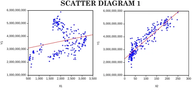
The table shows that all of the Independent Variables are significantly correlated to both Imports (y1) and Exports (y2) at . According to the Scatter Diagram below, two of the Independent variables, namely Exchange Rate and Domestic Crude Oil, are positively correlated. On the other hand, Inflation Rate and Interest Rate has a negative correlation to Imports. The Scatter Diagram of the Independent Variables to Import have a significant Linear relationship.
SCATTER DIAGRAM 1
1,000,000,000 2,000,000,000 3,000,000,000 4,000,000,000 5,000,000,000 6,000,000,000
500 1,000 1,500 2,000 2,500 3,000 3,500
X1
Y1
1,000,000,000 2,000,000,000 3,000,000,000 4,000,000,000 5,000,000,000 6,000,000,000
0 50 100 150 200 250 300
X2
Regression
1,000,000,000 2,000,000,000 3,000,000,000 4,000,000,000 5,000,000,000 6,000,000,000
0 2 4 6 8 10 12
X3
Y1
1,000,000,000 2,000,000,000 3,000,000,000 4,000,000,000 5,000,000,000 6,000,000,000
0 4 8 12 16 20 24 28
X4
Y1
In Exports, the Scatter Diagram shows that Exchange Rate and Domestic Crude Oil has a positive correlation to the Dependent variable while Inflation and Interest Rate both have a negative correlation to the Dependent variable. The scatter plots also shows that the Independent variables are significantly linear to
Export at .
SCATTER DIAGRAM 2
1,000,000,000 2,000,000,000 3,000,000,000 4,000,000,000 5,000,000,000 6,000,000,000
500 1,000 1,500 2,000 2,500 3,000 3,500
X1
Y2
1,000,000,000 2,000,000,000 3,000,000,000 4,000,000,000 5,000,000,000 6,000,000,000
0 50 100 150 200 250 300
X2
Y2
1,000,000,000 2,000,000,000 3,000,000,000 4,000,000,000 5,000,000,000 6,000,000,000
0 2 4 6 8 10 12
X3
Y2
1,000,000,000 2,000,000,000 3,000,000,000 4,000,000,000 5,000,000,000 6,000,000,000
0 4 8 12 16 20 24 28
X4
Mathematical Model formulated using Matrices through Normal Estimation Equation
The matrix theory was used to facilitate the mathematical manipulations since the researchers have more then two variables to fit Multiple Linear Regression. According to the multiple linear regression assumptions, these are the mathematical model that will predict the Dependent variables.
The least squares estimating equations (X’X) b=X’y
Thus, using b=(X’X)-1X’y to form the estimated regression
coefficients as: For Imports
b0=1701535913.57; b1=235974.045084;
b2=14789418.2525; b4=11067822.3757
For Exports
b0= -6426658579.74; b1=656926482.951;
b2=1029470376.45; b3=87112994.3622;
b4=208553220.498
Regression
One of the Independent variables is not significant to Imports which is Interest Rate while in Exports, there are two non-significant varibles which are Inflation Rate and Interest Rate. Then the researchers used MATLAB to formulate a mathematical model for Imports (y1) using its significant factors same as Exports (y2). To estimate Imports and Exports more precisely, the non-significant variables are excluded to the equation and a new mathematical model was formed:
Using the least squares estimating equations (X’X) b=X’y
Imports (y1)
b0 = 1529172628.02; b1 = 17936900.2752; b2 = 14215459.8761
Therefore Imports can be predicted through this regression equation:
Exports (y
2)
b0 = -5824275287.72; b1 = 663252302.938; b2 = 941801773.483
Significant factors that can predict Imports (y1) and
Exports (y2)
To identify the significant factors that affect the Dependent variables, the researchers used Eviews in conducting Multiple Linear Regression. Among the five (5) Independent variables namely: Exchange Rate (x1), Domestic Crude Oil (x2), Inflation Rate (x3) and Interest Rate (x4), only two Independent varibles are significant to Import (y1). These are Exchange Rate (x1) and Domestic Crude Oil (x2). While the transformed data of only two independent varibles are significant to Exports (y2) namely, Exchange Rate (lnx1) and Domestic Crude Oil (lnx2).
Significant difference of the Predicted Values from the
Actual Values of Imports (y1) and Exports (y2)
Paired T-test was used to analyze the difference between Actual and Predicted Values of Imports and Exports in the Philippines (See Appendix C: Table 10 & 12). The p-value of Imports and Exports results to 1.0000, which determine that there are no significant difference between the Actual and Predicted Value and the mathematical model will essentially predict the Imports and Exports in the Philippines.
Summary of Findings, Conclusions and
Recommendations
Summary of Findings
Behavior of the Graph of the Dependent and Independent Variables
Regression
fluctuates same goes for Inflation Rate and Interest Rate. But in Interest Rate it luctuates wildly. In the graph for Domestic Crude Oil, it noted its peak in June 2008 and fluctuates in February 2009 but then it continuously rises.
Significant Relationship between Dependent and Independent Variables
Upon using the Original data, the Independent variables are significantly correlated to both Imports and Exports based on Pearson’s coefficient of correlation. Since the null hypothesis of noramlity was rejected, the researchers used logarithmic transformation to transform the Independent variables. According to the result of Pearson’s coefficient correlation, the transformed Independet variables are still significantly correlated to Export.
Mathematical Model Formulated through Normal Estimation Equation
The first model estimate the Imports while the second model estimates Exports and both significant with a p-value of 0.0000. The coefficient of determination, also caled R-squared, of Imports (y1) is 0.880120 while Exports (y2) has 0.814517.
Significant Factors that Can Predict Imports (y1) and Exports (y2)
Significant Difference of the Predicted Values from the Actual Values of Imports (y1) and Exports (y2)
Paired t-test results to 1.000 for both Imports (x1) and Exports (x2) which is greater than the level of significance 0.01. Therefore, there is no significant difference between the Actual and Predicted Value of both Imports and Exports
Conclusions
The assumptions of Multiple Linear Regression were all satisfied. In the mathematical model of both the dependent variables, it shows that only two independent variables are significant to Imports (y1). These are: Exchange Rate (x1) and Domestic Crude Oil (x2). On the other hand, in Exports (y2), the logarithmic tranformation of only two independent varibles are significant namely: Exchange Rate (lny1) and Domestic Crude Oil (lny2). The mathematical model also shows that there are no significant difference between the Actual and Predicted value of both Import and Export.
Recommendations
The researchers propose looking for more independent variables such as: Foreign Direct Investment (FDI), Tariff Rate, Tranportation costs and Number of Employed. It also suggests in adding more series of data to assess Imports and Exports in the Philippines more accurately.
REFERENCES
Regression
[2]http://www.treasury.govt.nz/publications/researchpolicy/wp/2 012/12-05/08.htm Increased Export Demand
[3] http://www.idosi.org/mejsr/mejsr21%281%2914/30.pdf Muhammad Akbar Ali Shah, Muhammad Aleem & Nousheen Arshed. “Statistical Analysis of the Factors Affecting Inflation in Pakistan” Middle-East Journal of Scientific Research 21 (1): 181-189, 2014
[4]http://www.iiste.org/Journals/index.php/RJFA/article/viewFil e/7784/7922 Sajid Gul, Fakhra Malik & Nasir Razzaq (2013). “Factors Affecting the Demand Side of Exports: Pakistan Evidence” Research Journal of Finance and Accounting ISSN 2222-1697 (Paper) ISSN 2222-2847 (Online). Vol.4, No.13, 2013 [5] Yuhong Li, Zhongwen Chen & Xiaoyin Wang (2010). ”An Empirical Study on the Contribution of Foreign Trade to the Economic Growth of Jiangxi Province, China” iBusiness, 2010, 2, 183-187
[6]http://www.iosrjournals.org/iosr-jhss/papers/Vol14
issue6/K0146101106.pdf?id=6924 Dr Alam Raza, Dr Asadullah Larik, and Mr Muhammad Tariq (2013). “Effects of Currency Depreciation on Trade Balances of Developing Economies: A Comprehensive Study on South Asian Countries” IOSR Journal of Humanities and Social Science (IOSR-JHSS) Volume 14, Issue 6 (Sep. -Oct. 2013), PP 101-106
[7] http://library.iugaza.edu.ps/thesis/107822.pdf Mohammad A. N. Nassr (2013). “Determinants and Econometric Estimation of Imports Demand Function in Palestine” The Islamic University of Gaza Deanship of Higher Education Faculty of Commerce Master of Economic Development, 2013
[8]https://www.academia.edu/5647479/IMPACT_OF_RECESSI ON_ON_INDIA_S_EXPORT_AND_AFTERMATH_OF_GLOBA L_MELTDOWN
International Journal of Asian Research Consortium: Asian Journal of Research in Business Economics and Management. Volume 2; July 2012
[9]http://www.iiste.org/Journals/index.php/JEDS/article/viewFil e/7826/8001
Djoni, Dedi Darusman, Unang Atmaja, and Aziz Fauzi (2013). “Determinants of Indonesia’s Crude Coconut Oil Export Demand” Journal of Economics and Sustainable Development Vol.4, No.14, 2013
[10] Muhammad Bachal Jamali, Asif Shah, et.al. (2011). “Oil Price Shocks: A Comparative Study on the Impacts in Purchasing Power in Pakistan” Modern Applied Science Vol. 5, No. 2; April 2011
[11] http://www.aessweb.com/pdf-files/AJEM-2014-2%284%29-156-168.pdf Pamela F. Resurreccion (2014). “LINKING UNEMPLOYMENT TO INFLATION AND ECONOMIC GROWTH: TOWARD A BETTER UNDERSTANDING OF UNEMPLOYMENT IN THE PHILIPPINES” Asian Journal of Economic Modelling, 2014
[12] http://business.cardiff.ac.uk/sites/default/files/E2011_10.pdf Lucun Yang (2011). “An Empirical Analysis of Current Account Determinants in Emerging Asian Economies” Cardiff Economics Working Papers March 2011
[13]http://www.mbaskool.com/business-concepts/statistics/6914-multiple-regression.html Multiple Regression
[14]http://ncss.wpengine.netdna-cdn.com/wp
content/themes/ncss/pdf/Procedures/NCSS/Stepwise_Regression .pdf Chapter 311: Stepwise Regression. NCSS Statistical Software
Data Sources
Regression
Appendices
Appendix A
TABLE 1 Original Data
Date Import (y1) Export (y2) Exchange
Rate (x1)
Domestic Crude Oil (x2)
Inflation Rate (x3)
Interest Rate (x4)
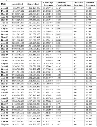
Jan-95 1,855,579,497 1,160,748,394 25.493714 31.67 6.1 8.886
Feb-95 1,615,887,292 1,263,768,380 25.133296 32.72 5.6 10.608
Mar-95 2,142,537,620 1,298,577,283 24.018913 32.55 6.0 19.266
Apr-95 2,229,563,126 1,377,417,699 23.601298 35.19 6.0 12.850
May-95 2,143,626,871 1,400,580,633 23.953675 34.55 6.2 9.909
Jun-95 2,328,664,433 1,521,691,870 23.763707 32.5 6.5 9.353
Jul-95 2,175,487,584 1,592,693,716 23.520389 30.1 6.3 7.585
Aug-95 2,273,585,811 1,591,446,955 24.260739 30.9 6.8 7.298
Sep-95 2,444,224,628 1,594,970,078 24.546892 31.42 8.0 8.250
Oct-95 2,342,361,497 1,601,650,105 23.923923 30.32 8.2 8.761
Nov-95 2,414,722,228 1,422,627,417 23.8939 31.51 8.4 12.342
Dec-95 2,571,385,721 1,621,013,605 24.250414 33.62 8.2 14.000
Jan-96 2,236,094,895 1,420,447,244 26.655576 33.34 9.5 13.975
Feb-96 2,359,578,155 1,594,005,715 26.739125 33.11 9.3 13.968
Mar-96 2,760,472,686 1,670,603,477 26.889452 36.4 9.5 13.870
Apr-96 2,811,146,347 1,491,866,914 27.229662 38.82 9.4 13.173
May-96 2,712,349,002 1,612,182,193 27.64238 35.76 9.2 12.320
Jun-96 2,750,550,811 1,793,390,815 27.499508 34.76 8.9 11.925
Jul-96 2,838,704,800 1,693,694,307 27.118984 36.63 8.7 11.666
Aug-96 2,799,675,243 1,773,892,603 26.851109 37.83 8.2 10.683
Sep-96 2,870,062,593 1,875,570,991 27.150647 41.47 6.7 11.450
Oct-96 2,858,505,702 1,883,709,477 27.380093 43.92 6.7 11.000
Nov-96 2,711,554,979 1,849,914,761 26.983619 41.73 6.6 10.857
Dec-96 2,718,238,732 1,883,267,902 27.560201 44.05 7.4 10.750
Jan-97 2,837,888,446 1,692,263,113 30.334677 43.63 5.4 10.543
Feb-97 2,626,538,787 1,812,415,070 31.678593 38.45 5.2 10.500
Mar-97 2,935,163,641 2,001,018,452 32.086308 36.4 5.5 10.170
Apr-97 2,942,077,383 2,082,429,845 32.2533 33.7 5.2 10.048
May-97 2,954,365,646 1,982,879,342 32.155345 36.52 5.0 15.788
Jun-97 3,032,341,153 2,129,077,284 32.488124 33.82 5.6 14.363
Jul-97 3,169,204,752 2,067,142,448 33.430851 34.59 5.6 25.720
Aug-97 3,327,943,486 2,257,973,088 34.428764 35.25 5.4 15.608
Sep-97 2,956,476,409 2,337,468,892 33.576302 35.13 5.7 12.000
Oct-97 3,413,800,271 2,326,046,764 32.964121 37.74 5.9 12.095
Nov-97 2,945,288,406 2,308,430,580 32.411972 35.96 6.7 12.000
Dec-97 2,792,733,044 2,230,557,752 33.212996 32.33 6.5 11.489
Jan-98 2,837,901,972 2,114,812,034 41.487237 28.18 6.6 12.370
Feb-98 2,585,234,573 2,227,202,908 41.486371 26.52 7.7 13.118
Mar-98 2,613,595,753 2,474,181,862 41.643433 24.74 8.2 13.000
Apr-98 2,457,455,132 2,284,501,468 41.40417 25.02 8.7 13.016
Jun-98 2,260,740,554 2,389,568,281 40.994605 23.39 10.2 13.125
Jul-98 2,465,592,507 2,501,374,868 41.146064 23.84 10.1 13.097
Aug-98 2,508,465,350 2,652,454,948 40.992774 23.44 10.1 16.734
Sep-98 2,454,452,775 2,786,324,139 39.132333 25.88 10.2 16.000
Oct-98 2,417,414,425 2,542,295,807 37.827966 24.89 10.0 13.945
Nov-98 2,373,400,659 2,585,815,298 38.781773 22.31 10.6 13.677
Dec-98 2,061,612,032 2,523,082,200 38.533371 19.54 10.0 13.375
Jan-99 2,399,845,062 2,580,780,826 39.283486 21.22 10.7 13.082
Feb-99 2,256,560,130 2,569,328,986 40.697939 20.14 9.3 12.500
Mar-99 2,656,303,584 2,702,330,690 41.909115 24.09 7.9 12.115
Apr-99 2,599,207,956 2,345,945,316 42.608674 29.49 7.4 11.018
May-99 2,533,475,252 2,746,896,905 42.915114 30.22 6.3 10.338
Jun-99 2,670,938,322 2,857,196,085 43.949121 30.45 5.3 9.476
Jul-99 2,791,640,360 2,851,061,303 44.069318 35.17 5.1 9.000
Aug-99 2,661,455,290 3,211,535,584 43.01561 37.92 4.8 9.000
Sep-99 2,555,295,681 3,693,275,081 43.436773 41.98 4.9 9.000
Oct-99 2,612,624,199 3,459,665,969 42.602214 41.66 5.2 9.000
Nov-99 2,351,642,775 3,075,370,095 44.122375 45.46 3.9 8.750
Dec-99 2,653,469,947 2,943,505,820 45.124302 46.91 3.9 8.750
Jan-00 2,900,849,185 2,716,571,560 43.806518 47.23 5.5 8.750
Feb-00 2,775,144,920 2,902,308,122 45.148686 50.85 5.6 8.750
Mar-00 2,908,071,277 2,988,516,721 46.038576 51.48 5.9 8.750
Apr-00 2,728,169,303 2,667,587,635 46.897639 43.95 6.2 8.750
May-00 2,641,931,449 2,930,834,998 48.793117 51.06 6.5 9.468
Jun-00 2,730,329,347 3,410,273,546 42.769928 55.5 6.1 10.000
Jul-00 2,855,651,733 3,219,402,685 44.515095 52.78 6.5 10.000
Aug-00 2,842,449,582 3,529,461,791 45.115379 55.12 6.8 10.000
Sep-00 3,294,233,553 3,502,006,958 45.829419 60.14 6.5 10.761
Oct-00 3,276,141,087 3,398,137,887 48.566885 58.93 6.7 13.198
Nov-00 2,919,802,695 3,316,782,069 49.9514 60.6 7.8 15.000
Dec-00 2,618,099,089 3,496,365,822 50.158102 35.76 8.7 13.881
Jan-01 3,031,155,224 2,888,995,982 51.343668 34.76 5.8 12.843
Feb-01 2,482,110,685 2,805,471,748 48.45399 36.63 5.8 11.172
Mar-01 3,037,402,171 2,869,640,382 48.496592 37.83 5.8 10.462
Apr-01 3,105,061,460 2,245,694,300 50.549373 41.47 5.5 9.829
May-01 2,939,857,616 2,599,971,007 50.734209 43.92 5.5 9.213
Jun-01 2,856,881,764 2,578,163,835 51.746767 41.73 5.9 9.000
Jul-01 2,873,159,620 2,594,446,005 53.554883 44.05 6.0 9.000
Aug-01 2,893,639,222 2,620,764,527 52.08795 43.63 5.7 9.000
Sep-01 2,752,002,754 2,731,019,845 51.489018 38.45 5.7 9.000
Oct-01 2,540,952,151 2,940,767,411 51.882151 36.4 5.2 8.803
Nov-01 2,216,795,607 2,629,794,168 51.942137 33.7 4.2 8.357
Dec-01 2,328,142,161 2,645,473,482 51.774882 36.52 3.7 7.951
Jan-02 2,225,785,816 2,631,435,355 51.246655 33.82 3.3 7.644
Feb-02 2,543,971,218 2,627,871,195 51.254533 34.59 2.9 7.386
Mar-02 3,435,733,641 2,849,061,701 51.044663 35.25 3.3 7.134
Apr-02 3,881,243,822 2,748,802,011 50.931722 35.13 3.4 7.000
May-02 3,302,515,506 2,918,058,836 49.824462 37.74 3.2 7.000
Regression
Sep-02 3,536,524,609 3,191,393,763 52.116933 53.05 2.5 7.000
Oct-02 3,247,166,736 3,033,181,410 52.9387 51.64 2.3 7.000
Nov-02 3,436,504,924 3,103,283,089 53.335651 46.49 2.1 7.000
Dec-02 2,896,396,477 2,913,746,779 53.45466 52.27 2.1 7.000
Jan-03 3,142,485,095 2,732,849,831 53.622681 57.64 1.9 7.000
Feb-03 3,021,435,800 2,787,824,284 54.148417 61.6 2.3 7.000
Mar-03 3,694,218,185 3,128,981,051 55.518177 56.83 2.1 7.000
Apr-03 3,432,718,138 2,726,211,859 53.869483 47.75 2.2 7.000
May-03 3,609,650,172 2,827,660,315 52.290712 48.85 2.2 7.000
Jun-03 3,175,460,334 3,060,470,078 53.457274 52.26 2.8 7.000
Jul-03 3,491,615,410 3,009,494,255 53.592786 53.59 2.3 6.761
Aug-03 3,360,194,190 3,003,210,820 55.009914 55.63 2.2 6.750
Sep-03 3,265,383,065 3,353,950,818 54.857617 50.42 2.2 6.750
Oct-03 3,401,221,235 3,339,920,475 54.832716 54.41 2.3 6.750
Nov-03 3,545,748,924 3,085,491,785 55.405825 54.61 2.4 6.750
Dec-03 3,330,381,135 3,175,139,873 55.276958 56.14 2.5 6.750
Jan-04 3,481,404,008 2,849,366,652 55.544329 58.74 2.9 6.750
Feb-04 3,313,652,857 3,004,810,087 56.017334 58.65 2.9 6.750
Mar-04 3,921,992,789 3,361,747,792 56.509691 63.02 3.1 6.750
Apr-04 3,764,804,339 2,982,491,297 56.536454 63.16 3.2 6.750
May-04 3,583,997,105 3,267,549,867 55.777748 70.37 3.6 6.750
Jun-04 3,778,070,418 3,317,928,115 55.994516 66.64 4.1 6.750
Jul-04 3,760,773,676 3,108,881,144 55.741021 70.96 5.5 6.750
Aug-04 3,687,633,143 3,430,059,627 55.846452 78.83 5.7 6.750
Sep-04 3,816,873,705 3,641,425,821 56.232977 77.73 6.2 6.750
Oct-04 4,007,923,809 3,753,434,618 56.342479 87.38 6.3 6.750
Nov-04 3,657,579,571 3,685,405,864 56.285678 78.61 6.8 6.750
Dec-04 3,264,507,024 3,277,419,596 56.175847 73.02 7.1 6.750
Jan-05 3,501,396,118 3,294,323,624 55.687054 80.38 7.3 6.750
Feb-05 3,211,228,572 3,000,164,622 54.774704 83.2 7.3 6.750
Mar-05 3,832,010,849 3,267,571,826 54.401201 95.37 7.1 6.750
Apr-05 4,112,555,946 3,245,696,520 54.432355 94.94 7.2 6.956
May-05 3,797,998,517 3,304,994,276 54.329855 89.71 7.3 7.000
Jun-05 4,210,263,190 3,358,573,683 55.259998 101.1 6.7 7.000
Jul-05 3,832,986,991 3,503,070,371 56.001773 105.71 6.0 7.000
Aug-05 4,238,873,900 3,512,640,841 55.943745 115.97 6.1 7.000
Sep-05 4,337,202,046 3,674,931,488 56.119012 115.58 6.0 7.082
Oct-05 4,159,123,833 3,634,525,359 55.581563 109.02 6.2 7.342
Nov-05 3,975,165,387 3,631,007,906 54.520688 103.18 6.2 7.500
Dec-05 4,209,377,205 3,827,182,953 53.521415 105.83 5.9 7.500
Jan-06 3,707,182,989 3,532,749,442 52.541075 117.1 5.9 7.500
Feb-06 3,415,251,347 3,448,303,896 51.745293 112.09 6.5 7.500
Mar-06 4,226,604,784 4,173,597,607 51.164396 114.32 6.6 7.500
Apr-06 4,416,675,003 3,917,884,768 51.399936 127.6 6.3 7.500
May-06 4,447,840,897 3,885,116,437 52.170252 128.85 6.0 7.500
Jun-06 4,533,998,702 4,055,141,466 53.170687 128.15 5.9 7.500
Jul-06 4,412,450,654 4,016,282,591 52.265336 135.97 5.5 7.500
Aug-06 4,883,658,015 4,273,802,974 51.292676 134.81 5.2 7.500
Sep-06 4,355,481,743 4,178,404,907 50.30806 116.62 4.9 7.500
Oct-06 4,686,409,641 4,207,335,417 49.974162 108.78 4.7 7.500
Dec-06 4,178,473,968 3,690,464,643 49.401492 114.52 4.1 7.500
Jan-07 3,904,161,111 3,991,848,889 48.891518 100.52 3.8 7.500
Feb-07 3,690,137,256 3,721,345,093 48.314726 108.08 2.9 7.500
Mar-07 4,566,515,375 4,487,333,472 48.384367 113.85 2.6 7.500
Apr-07 4,342,796,679 4,124,048,820 47.664218 122.28 2.6 7.500
May-07 4,296,137,369 4,127,864,486 46.72586 122.52 2.7 7.500
Jun-07 4,706,535,408 4,147,420,772 46.181655 128.08 2.6 7.500
Jul-07 5,041,563,307 4,248,793,462 45.51051 138.12 2.9 6.552
Aug-07 4,986,612,367 4,121,450,834 46.149121 131.63 2.7 6.000
Sep-07 4,743,796,494 4,389,378,756 45.999243 144.05 2.9 6.000
Oct-07 5,150,645,086 4,659,530,169 44.207622 153.84 2.9 5.799
Nov-07 5,084,213,106 3,964,806,575 43.091168 171.38 3.1 5.613
Dec-07 5,000,629,663 4,481,902,591 41.561263 168.05 3.7 5.445
Jan-08 4,995,763,280 4,230,559,185 40.821496 170.25 4.6 5.232
Feb-08 4,491,460,270 4,112,011,705 40.5793 175.34 5.1 5.000
Mar-08 5,123,010,793 4,200,129,457 41.234754 191.1 5.9 5.000
Apr-08 4,856,957,640 4,327,475,585 41.770219 204.24 7.3 5.000
May-08 4,775,682,154 4,225,382,102 42.997373 230.52 8.2 5.000
Jun-08 5,322,249,868 4,527,022,129 44.302383 247.01 9.4 5.212
Jul-08 5,882,357,556 4,437,234,124 44.827868 249.66 10.2 5.490
Aug-08 5,044,108,186 4,394,497,148 44.95862 215.3 10.5 5.778
Sep-08 4,891,088,820 4,445,618,966 46.70882 187.06 10.1 6.000
Oct-08 4,577,741,128 3,990,058,305 47.977344 136.34 9.7 6.000
Nov-08 3,484,679,377 3,512,973,480 49.087992 101.24 9.1 6.000
Dec-08 3,300,961,298 2,674,578,323 47.998288 77.71 7.8 5.825
Jan-09 3,269,937,726 2,512,962,951 47.101828 82.58 7.1 5.450
Feb-09 3,058,781,168 2,506,323,003 47.584664 78.83 7.2 5.000
Mar-09 3,269,832,510 2,906,745,064 48.362602 87.89 6.6 4.781
Apr-09 3,057,230,958 2,803,772,063 48.115128 94.55 5.6 4.616
May-09 3,616,585,310 3,088,029,755 47.328023 109.28 4.3 4.475
Jun-09 4,106,944,174 3,406,912,732 47.82949 129.99 3.2 4.250
Jul-09 4,025,962,245 3,313,362,062 48.07349 121.64 2.2 4.071
Aug-09 3,617,293,198 3,472,893,225 48.222279 134.68 1.7 4.000
Sep-09 3,669,908,170 3,637,638,407 48.053827 128.47 2.3 4.000
Oct-09 3,808,286,396 3,748,094,991 46.852989 139.21 2.9 4.000
Nov-09 3,654,514,062 3,717,828,961 47.041493 145.82 3.5 4.000
Dec-09 3,936,259,964 3,321,242,946 46.331693 140.86 4.4 4.000
Jan-10 4,310,255,692 3,579,440,238 46.038862 144.95 3.9 4.000
Feb-10 3,906,250,414 3,570,228,465 46.26492 140.4 3.9 4.000
Mar-10 4,555,823,918 4,181,803,677 45.692763 148.94 3.9 4.000
Apr-10 4,568,356,276 3,611,608,900 44.599005 158.13 4.0 4.000
May-10 4,811,756,231 4,241,422,444 45.625736 142.15 3.9 4.000
Jun-10 4,224,948,879 4,556,729,367 46.358678 140.45 3.6 4.000
Jul-10 4,687,766,029 4,505,187,660 46.255086 139.96 3.7 4.000
Aug-10 4,461,161,269 4,774,445,446 45.172882 142.57 4.1 4.000
Sep-10 4,597,217,542 5,340,846,922 44.216796 143.08 3.8 4.000
Oct-10 4,904,460,728 4,788,452,359 43.378653 153.57 3.3 4.000
Nov-10 4,955,778,246 4,146,073,638 43.557046 158.91 3.7 4.000
Regression
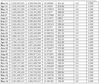
Mar-11 5,552,507,651 4,356,350,530 43.485661 204.42 4.9 4.062
Apr-11 5,525,435,059 4,306,444,209 43.18256 218.82 4.7 4.250
May-11 4,892,571,282 4,118,691,412 43.179919 203.62 4.9 4.462
Jun-11 4,503,899,301 4,134,781,698 43.41677 199.35 5.2 4.500
Jul-11 5,001,324,831 4,460,269,870 42.737966 203.23 4.9 4.500
Aug-11 5,076,381,479 4,172,903,202 42.414871 189.5 4.6 4.500
Sep-11 5,082,890,815 3,896,952,089 43.090347 190.27 4.7 4.500
Oct-11 5,024,485,134 4,155,662,784 43.352412 188.44 5.2 4.500
Nov-11 5,024,010,143 3,366,029,692 43.33757 198.51 4.7 4.500
Dec-11 4,633,315,515 3,407,157,204 43.661404 196.31 4.2 4.500
Jan-12 5,139,403,837 4,123,420,986 43.560124 201.32 4.0 4.410
Feb-12 4,998,181,721 4,430,449,373 42.663933 212.38 2.7 4.250
Mar-12 5,371,483,010 4,324,619,800 42.901125 222.03 2.6 4.000
Apr-12 4,788,116,423 4,635,171,810 42.657951 214.36 3.0 4.000
May-12 5,385,843,569 4,931,595,660 42.941953 196.28 3.0 4.000
Jun-12 5,103,026,146 4,314,231,994 42.720077 171.02 2.9 4.000
Jul-12 5,047,279,934 4,727,394,926 41.87161 182.28 3.2 3.960
Aug-12 5,183,825,724 3,809,977,241 42.074267 198.42 3.8 3.750
Sep-12 5,326,588,737 4,810,795,438 41.717493 200.48 3.7 3.750
Oct-12 5,276,855,131 4,410,108,337 41.383135 195.06 3.2 3.500
Nov-12 5,207,737,397 3,611,009,789 41.096239 190.93 2.8 3.500
Dec-12 5,300,315,989 3,970,745,308 41.004599 190.81 3.0 3.500
Jan-13 4,727,031,391 4,010,779,236 40.717713 197.91 3.1 3.500
Feb-13 4,707,488,493 3,740,782,025 40.688326 202.94 3.4 3.500
Mar-13 4,921,836,577 4,328,976,422 40.739739 193.35 3.2 3.500
Apr-13 5,141,343,971 4,121,281,122 41.186047 186.21 2.6 3.500
May-13 5,257,805,111 4,893,276,517 41.361491 186.98 2.6 3.500
TABLE 2
Transformed Data
Date LNX1 LNX2 Date LNX1 LNX2
Jan-95 6.48 3.46 Jan-98 7.45 3.34
Feb-95 6.45 3.49 Feb-98 7.45 3.28
Mar-95 6.36 3.48 Mar-98 7.46 3.21
Apr-95 6.32 3.56 Apr-98 7.45 3.22
May-95 6.35 3.54 May-98 7.41 3.26
Jun-95 6.34 3.48 Jun-98 7.43 3.15
Jul-95 6.32 3.4 Jul-98 7.43 3.17
Aug-95 6.38 3.43 Aug-98 7.43 3.15
Sep-95 6.4 3.45 Sep-98 7.33 3.25
Oct-95 6.35 3.41 Oct-98 7.27 3.21
Nov-95 6.35 3.45 Nov-98 7.32 3.11
Dec-95 6.38 3.52 Dec-98 7.3 2.97
Jan-96 6.57 3.51 Jan-99 7.34 3.05
Feb-96 6.57 3.5 Feb-99 7.41 3
Mar-96 6.58 3.59 Mar-99 7.47 3.18
Apr-96 6.61 3.66 Apr-99 7.5 3.38
May-96 6.64 3.58 May-99 7.52 3.41
Jun-96 6.63 3.55 Jun-99 7.57 3.42
Aug-96 6.58 3.63 Aug-99 7.52 3.64
Sep-96 6.6 3.72 Sep-99 7.54 3.74
Oct-96 6.62 3.78 Oct-99 7.5 3.73
Nov-96 6.59 3.73 Nov-99 7.57 3.82
Dec-96 6.63 3.79 Dec-99 7.62 3.85
Jan-97 6.82 3.78 Jan-00 7.56 3.86
Feb-97 6.91 3.65 Feb-00 7.62 3.93
Mar-97 6.94 3.59 Mar-00 7.66 3.94
Apr-97 6.95 3.52 Apr-00 7.7 3.78
May-97 6.94 3.6 May-00 7.78 3.93
Jun-97 6.96 3.52 Jun-00 7.51 4.02
Jul-97 7.02 3.54 Jul-00 7.59 3.97
Aug-97 7.08 3.56 Aug-00 7.62 4.01
Sep-97 7.03 3.56 Sep-00 7.65 4.1
Oct-97 6.99 3.63 Oct-00 7.77 4.08
Nov-97 6.96 3.58 Nov-00 7.82 4.1
Dec-97 7.01 3.48 Dec-00 7.83 3.58
Date LNX1 LNX2 Date LNX1 LNX2
Jan-01 7.88 3.55 Mar-04 8.07 4.14
Feb-01 7.76 3.6 Apr-04 8.07 4.15
Mar-01 7.76 3.63 May-04 8.04 4.25
Apr-01 7.85 3.72 Jun-04 8.05 4.2
May-01 7.85 3.78 Jul-04 8.04 4.26
Jun-01 7.89 3.73 Aug-04 8.05 4.37
Jul-01 7.96 3.79 Sep-04 8.06 4.35
Aug-01 7.91 3.78 Oct-04 8.06 4.47
Sep-01 7.88 3.65 Nov-04 8.06 4.36
Oct-01 7.9 3.59 Dec-04 8.06 4.29
Nov-01 7.9 3.52 Jan-05 8.04 4.39
Dec-01 7.89 3.6 Feb-05 8.01 4.42
Jan-02 7.87 3.52 Mar-05 7.99 4.56
Feb-02 7.87 3.54 Apr-05 7.99 4.55
Mar-02 7.87 3.56 May-05 7.99 4.5
Apr-02 7.86 3.56 Jun-05 8.02 4.62
May-02 7.82 3.63 Jul-05 8.05 4.66
Jun-02 7.84 3.58 Aug-05 8.05 4.75
Jul-02 7.85 3.48 Sep-05 8.05 4.75
Aug-02 7.89 3.34 Oct-05 8.04 4.69
Sep-02 7.91 3.97 Nov-05 8 4.64
Oct-02 7.94 3.94 Dec-05 7.96 4.66
Nov-02 7.95 3.84 Jan-06 7.92 4.76
Dec-02 7.96 3.96 Feb-06 7.89 4.72
Jan-03 7.96 4.05 Mar-06 7.87 4.74
Feb-03 7.98 4.12 Apr-06 7.88 4.85
Mar-03 8.03 4.04 May-06 7.91 4.86
Apr-03 7.97 3.87 Jun-06 7.95 4.85
May-03 7.91 3.89 Jul-06 7.91 4.91
Jun-03 7.96 3.96 Aug-06 7.88 4.9
Regression
Oct-03 8.01 4 Dec-06 7.8 4.74
Nov-03 8.03 4 Jan-07 7.78 4.61
Dec-03 8.02 4.03 Feb-07 7.76 4.68
Jan-04 8.03 4.07 Mar-07 7.76 4.73
Feb-04 8.05 4.07 Apr-07 7.73 4.81
Date LNX1 LNX2 Date LNX1 LNX2
May-07 7.69 4.81 Jun-10 7.67 4.94
Jun-07 7.67 4.85 Jul-10 7.67 4.94
Jul-07 7.64 4.93 Aug-10 7.62 4.96
Aug-07 7.66 4.88 Sep-10 7.58 4.96
Sep-07 7.66 4.97 Oct-10 7.54 5.03
Oct-07 7.58 5.04 Nov-10 7.55 5.07
Nov-07 7.53 5.14 Dec-10 7.56 5.13
Dec-07 7.45 5.12 Jan-11 7.58 5.16
Jan-08 7.42 5.14 Feb-11 7.55 5.22
Feb-08 7.41 5.17 Mar-11 7.54 5.32
Mar-08 7.44 5.25 Apr-11 7.53 5.39
Apr-08 7.46 5.32 May-11 7.53 5.32
May-08 7.52 5.44 Jun-11 7.54 5.3
Jun-08 7.58 5.51 Jul-11 7.51 5.31
Jul-08 7.61 5.52 Aug-11 7.49 5.24
Aug-08 7.61 5.37 Sep-11 7.53 5.25
Sep-08 7.69 5.23 Oct-11 7.54 5.24
Oct-08 7.74 4.92 Nov-11 7.54 5.29
Nov-08 7.79 4.62 Dec-11 7.55 5.28
Dec-08 7.74 4.35 Jan-12 7.55 5.3
Jan-09 7.7 4.41 Feb-12 7.51 5.36
Feb-09 7.73 4.37 Mar-12 7.52 5.4
Mar-09 7.76 4.48 Apr-12 7.51 5.37
Apr-09 7.75 4.55 May-12 7.52 5.28
May-09 7.71 4.69 Jun-12 7.51 5.14
Jun-09 7.74 4.87 Jul-12 7.47 5.21
Jul-09 7.75 4.8 Aug-12 7.48 5.29
Aug-09 7.75 4.9 Sep-12 7.46 5.3
Sep-09 7.74 4.86 Oct-12 7.45 5.27
Oct-09 7.69 4.94 Nov-12 7.43 5.25
Nov-09 7.7 4.98 Dec-12 7.43 5.25
Dec-09 7.67 4.95 Jan-13 7.41 5.29
Jan-10 7.66 4.98 Feb-13 7.41 5.31
Feb-10 7.67 4.94 Mar-13 7.41 5.26
Mar-10 7.64 5 Apr-13 7.44 5.23
Apr-10 7.6 5.06 May-13 7.44 5.23
Appendix B
Imports (y1)
GRAPH 1
Testing for Normality
0 4 8 12 16 20
-5.0e+08 500.000 5.0e+08 1.0e+09
Series: Residuals Sample 1995M01 2013M05 Observations 221
Mean -3.40e-07 Median 265283.6 Maximum 1.00e+09 Minimum -8.57e+08 Std. Dev. 3.43e+08 Skewness 0.032206 Kurtosis 2.948999
Jarque-Bera 0.062157 Probability 0.969400
H0: The data have a normal distribution
Ha: The data does not have a normal distribution
Rejection Rule: If p-value < , then reject the null hypothesis.
Conclusion
Since the p-value, 0.969400, is greater than 0.01, then FAIL TO REJECT the null hypothesis for the Jarque-Bera Test. Therefore, the data have a normal distribution.
TABLE 3
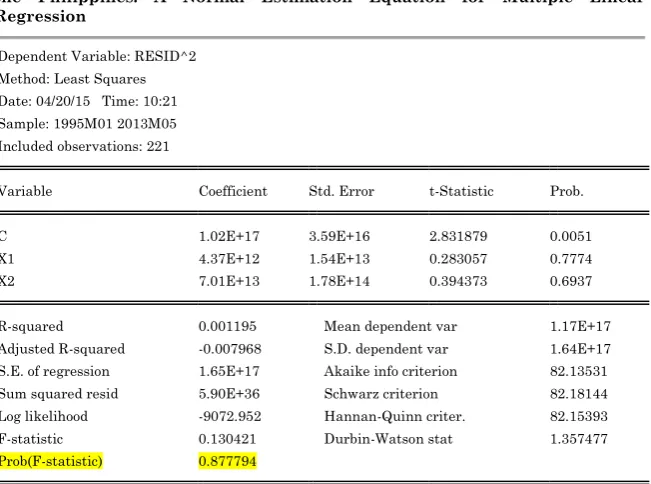
Testing for Homoscedasticity
Heteroskedasticity Test: Breusch-Pagan-Godfrey
Regression
Dependent Variable: RESID^2 Method: Least Squares Date: 04/20/15 Time: 10:21 Sample: 1995M01 2013M05 Included observations: 221
Variable Coefficient Std. Error t-Statistic Prob.
C 1.02E+17 3.59E+16 2.831879 0.0051
X1 4.37E+12 1.54E+13 0.283057 0.7774
X2 7.01E+13 1.78E+14 0.394373 0.6937
R-squared 0.001195 Mean dependent var 1.17E+17 Adjusted R-squared -0.007968 S.D. dependent var 1.64E+17 S.E. of regression 1.65E+17 Akaike info criterion 82.13531 Sum squared resid 5.90E+36 Schwarz criterion 82.18144 Log likelihood -9072.952 Hannan-Quinn criter. 82.15393 F-statistic 0.130421 Durbin-Watson stat 1.357477 Prob(F-statistic) 0.877794
H0: The variables are Homoscedastic
Ha: The variables are Heteroscedastic
Rejection Rule: If p-value < , then reject the null hypothesis
Conclusion
Since the p-value, 0.877794, is greater than 0.01, then FAIL TO REJECT the null hypothesis for the Breusch-Pagan-Godfrey Heteroscedasticity Test. Therefore, the variables are Homoscedastic.
TABLE 4
Testing for Multicollinearity
Variance Inflation Factors Date: 04/20/15 Time: 10:27 Sample: 1995M01 2013M05 Included observations: 221
Coefficient Uncentered Centered
C 5.66E+15 10.52809 NA
X1 1.04E+09 9.204268 1.010292
X2 1.39E+11 3.199333 1.010292
General Rule: For satisfying Multicollinearity, the Variance Inflation Factor should be less than 10.
Conclusion
Since the VIF (Variance Inflation Factor) of the following independent variables are less than 10 therefore the Assumption, Multicollinearity, was satisfied.
TABLE 5
Testing for Linearity
Dependent Variable: Y1 Method: Least Squares Date: 04/20/15 Time: 20:06 Sample: 1995M01 2013M05 Included observations: 221
Variable Coefficient Std. Error t-Statistic Prob.
C 1.86E+09 75211624 24.79644 0.0000
X1 218424.5 32310.87 6.760094 0.0000
X2 14357624 372468.7 38.54720 0.0000
R-squared 0.880120 Mean dependent var 3.64E+09 Adjusted R-squared 0.879021 S.D. dependent var 9.91E+08 S.E. of regression 3.45E+08 Akaike info criterion 42.16711 Sum squared resid 2.59E+19 Schwarz criterion 42.21324 Log likelihood -4656.465 Hannan-Quinn criter. 42.18573 F-statistic 800.2456 Durbin-Watson stat 0.766682 Prob(F-statistic) 0.000000
H0: No Independent variables that is significant to the Dependent variable.
Ha: At least one of the Independent variables will be significant to the
Regression
Rejection Rule: If p-value < , then reject the null hypothesis
Conclusion
Since the p-value, 0.000000, is less than 0.01, then REJECT the null hypothesis. Therefore, at least one of the Independent variables will be significant to the Dependent variables.
Exports (y2)
TABLE 6
Testing for Multicollinearity
Variance Inflation Factors Date: 04/20/15 Time: 10:47 Sample: 1995M01 2013M05 Included observations: 221
Coefficient Uncentered Centered
Variable Variance VIF VIF
C 1.97E+17 279.0873 NA
LNX1 3.86E+15 312.9747 1.122523 LNX2 1.56E+15 41.53851 1.122523
General Rule: For satisfying Multicollinearity, the Variance Inflation Factor should be less than 10
Conclusion
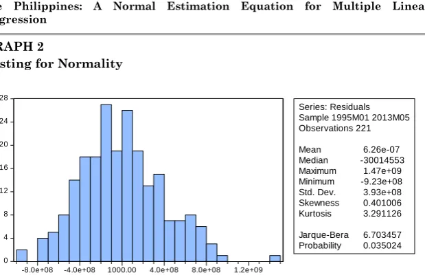
GRAPH 2
Testing for Normality
0 4 8 12 16 20 24 28
-8.0e+08 -4.0e+08 1000.00 4.0e+08 8.0e+08 1.2e+09
Series: Residuals Sample 1995M01 2013M05 Observations 221
Mean 6.26e-07 Median -30014553 Maximum 1.47e+09 Minimum -9.23e+08 Std. Dev. 3.93e+08 Skewness 0.401006 Kurtosis 3.291126
Jarque-Bera 6.703457 Probability 0.035024
H0: The data have a normal distribution
Ha: The data does not have a normal distribution
Rejection Rule: If p-value < , then reject the null hypothesis
Conclusion
Since the p-value, 0.035024 is greater than 0.01, then FAIL TO REJECT the null hypothesis for the Jarque-Bera Test. Therefore, the data have a normal distribution.
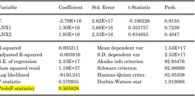
TABLE 7
Testing for Homoscedasticity
Heteroskedasticity Test: Breusch-Pagan-Godfrey
F-statistic 0.570955 Prob. F(2,218) 0.5658 Obs*R-squared 1.151593 Prob. Chi-Square(2) 0.5623 Scaled explained SS 1.283649 Prob. Chi-Square(2) 0.5263
Test Equation:
Regression
Sample: 1995M01 2013M05 Included observations: 221
Variable Coefficient Std. Error t-Statistic Prob.
C -2.79E+16 2.62E+17 -0.106226 0.9155
LNX1 1.30E+16 3.68E+16 0.353757 0.7239
LNX2 1.95E+16 2.33E+16 0.834855 0.4047
R-squared 0.005211 Mean dependent var 1.54E+17 Adjusted R-squared -0.003916 S.D. dependent var 2.33E+17 S.E. of regression 2.33E+17 Akaike info criterion 82.83476 Sum squared resid 1.19E+37 Schwarz criterion 82.88089 Log likelihood -9150.241 Hannan-Quinn criter. 82.85338 F-statistic 0.570955 Durbin-Watson stat 1.018068 Prob(F-statistic) 0.565828
H0: The variables are Homoscedastic
Ha: The variables are Heteroscedastic
Rejection Rule: If p-value < , then reject the null hypothesis
Conclusion
Since the p-value, 0.565828 is greater than 0.01, then FAIL TO REJECT the null hypothesis for the Breusch-Pagan-Godfrey Heteroscedasticity Test. Therefore, the variables are Homoscedastic.
TABLE 8
Testing for Linearity
Dependent Variable: Y2 Method: Least Squares Date: 04/20/15 Time: 10:44 Sample: 1995M01 2013M05 Included observations: 221
Variable Coefficient Std. Error t-Statistic Prob.
C -5.82E+09 4.43E+08 -13.13535 0.0000
LNX2 9.42E+08 39446723 23.87529 0.0000
R-squared 0.814429 Mean dependent var 3.21E+09 Adjusted R-squared 0.812726 S.D. dependent var 9.12E+08 S.E. of regression 3.95E+08 Akaike info criterion 42.43798 Sum squared resid 3.39E+19 Schwarz criterion 42.48411 Log likelihood -4686.397 Hannan-Quinn criter. 42.45661 F-statistic 478.3762 Durbin-Watson stat 0.580259 Prob(F-statistic) 0.000000
H0: No Independent variables that is significant to the Dependent variable.
Ha: At least one of the Independent variables will be significant to the
Dependent variable.
Rejection Rule: If p-value < , then reject the null hypothesis
Conclusion
Since the p-value, 0.000000, is less than 0.01, then REJECT the null hypothesis. Therefore, at least one of the Independent variables will be significant to the Dependent variables.
APPENDIX C
Difference between Actual and Predicted Value
TABLE 9 (Imports)
Actual Value Predicted Value Difference of Actual and Predicted Value 1855579497 2461647006 -606067508.8
Regression
Regression
Regression
5302439096 4794494622 507944474.4 4876579960 4924096559 -47516598.84 5552507651 5213007334 339500316.7 5525435059 5414019254 111415804.7 4892571282 5195733571 -303162288.6 4503899301 5138906524 -635007222.6 5001324831 5181840149 -180515318.1 5076381479 4978700591 97680888.22 5082890815 5002371453 80519361.96 5024485134 4981045113 43440020.73 5024010143 5125345337 -101335193.9 4633315515 5099912294 -466596779.4 5139403837 5169914465 -30510628.04 4998181721 5311831394 -313649672.8 5371483010 5454815457 -83332447.06 4788116423 5340148004 -552031580.7 5385843569 5085872208 299971360.8 5103026146 4719047204 383978942 5047279934 4865036986 182242947.8 5183825724 5100484905 83340819.44 5326588737 5123531863 203056874.2 5276855131 5039644540 237210591 5207737397 4975178975 232558422.1 5300315989 4971812694 328503295 4727031391 5068630852 -341599460.5 4707488493 5140327161 -432838667.8 4921836577 5003551986 -81715408.68 5141343971 4909025068 232318902.6 5257805111 4923243767 334561344.4
TABLE 10
Hypothesis Testing for DIFF1 Date: 04/29/15 Time: 17:27 Sample: 1 221
Included observations: 221
Test of Hypothesis: Mean = 0.000000
Sample Mean = -0.002154 Sample Std. Dev. = 3.43e+08
Method Value Probability
TABLE 11 (Exports)
Actual Value Predicted Value
Difference of
Actual and
Regression
Regression
Regression
TABLE 12
Hypothesis Testing for DIFF2 Date: 04/29/15 Time: 17:35 Sample: 1 221
Included observations: 221
Test of Hypothesis: Mean = 0.000000
Sample Mean = 0.002800 Sample Std. Dev. = 3.93e+08
Method Value Probability