Design and Implementation of Electro Mechanical Actuator Control System

(1)

International Journal of Research (IJR)

e-ISSN: 2348-6848, p- ISSN: 2348-795X Volume 2, Issue 10, October 2015

Available at http://internationaljournalofresearch.org

Design and Implementation of Electro Mechanical Actuator

Control System

Bollam Seetharama Lakshmi

(Gandhiji Institute Of Science And Technology)

H.NO: 13JF1D6804

Guide:

B. S. Madhuri

(M-Tech)

H. O .D:

S. Neelima

(M-Tech)

ABSTRACT

In this paper recent control developments for an electromechanical valve actuator will be presented. The model-based control methodology utilizes position feedback, a nonlinear observer that provides virtual sensing of the armature velocity and current, and cycle-to-cycle learning. The controller is based on a nonlinear state-space description of the actuator that is derived based on physical principles and parameter identification. A bench- top experimental setup and a rapid control prototyping system are used to quantify the actuator performance. Experiments are conducted to measure valve release timing, transition times, and contact velocities for open- and closed-loop control schemes. Simulation results are presented for a feed-forward cycle-to-cycle learning controller.

INTRODUCTION

Electro-Mechanical Valve (EMV) actuators shown in Fig.1 are currently being developed by many engine and component manufacturers. These actuators can potentially improve engine performance via flexibility in valves timings at all engine operating conditions. Unlike conventional camshaft driven systems, EMV system affords valve timings that are fully independent of crankshaft position. The additional flexibility in valve timing gives excellent cycle-to-cycle control of cylinder air charge and residual gas fractions. Fuel economy can be improved through unthrottled load control and cylinder deactivation. Internal residuals together with appropriate valve actuation schemes can be used to lower exhaust emissions below engines with a camshaft. At low-to-moderate engine speeds, valve timings can be optimized to improve full load torque.

Although a conventional valvetrain system limits engine performance, it has operational advantages. The valve motion is controlled by a cam profile that is carefully designed to give low seating velocities for durability and low noise. In contrast, an EMV system introduces a difficult motion control problem. Accurate valve timings,

fast transitions, and low seating velocities (soft landing) must be achieved. Robust soft landing control is required before EMV systems are introduced into the market.

EMV actuator assembly with valve shown inopen position.

The difficulty in achieving soft landing stems from several factors:

1. Requirements for low landing velocity (< 0.1 m/sec at 1500 rpm)

2. Requirements for fast transition times (≈ 3.5 ms) 3. Net power losses must be similar to

conventional cam drive system

4. Affordable sensors for robust feedback control 5. Highly nonlinear magnetic force characteristics 6. Limited range of actuator authority

(2)

International Journal of Research (IJR)

(3)

International Journal of Research (IJR)

a feed-forward cycle-to-cycle learning controller are also presented.

OVERVIEW OF THE EMV ACTUATOR SYSTEM

Fig. 1 shows a schematic of an EMV actuator mounted on a cylinder head. The actuator consists of a lower electromagnetic coil for opening the valve and an upper coil for closing the valve. Actuator and valve springs push on the armature and valve stem through spring retainers. At neutral position the actuator and valve springs are equally compressed and the armature is centered between the upper and lower coils. At start- up, a voltage is applied to one of the electromagnets to move the armature from neutral position to the fully open or fully closed position. A small holding voltage is then maintained to hold the armature in place against the spring force.

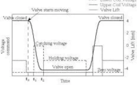
Fig. 2 shows valve position and coil voltages during standard operation. Consider the transition from open-to-closed position. A holding voltage is first applied to the lower coil. Releasing this holding voltage then allows the compressed spring to push on the armature and initiate the valve motion. A catching voltage is then applied to the upper coil to capture the armature in the upper position, and so on. After the initial start-up from the neutral position, the actuator is principally a spring-mass pendulum that is driven by an electromagnetic force. The potential energy is transferred between the two springs via the armature and valve. A catching voltage is applied to the appropriate coil to inject enough magnetic energy to overcome the losses from friction forces, gas flow forces, and possibly magnetic forces from the releasing coil.

A schematic of the electro-mechanical valveopening and closing and commanded voltage.

The mechanical spring force and the magnetic force largely determine the actuator and valve operation. As such, an analysis of the complete system must consider

interactions among the electrical, magnetic, and mechanical subsystems. Since the valve opening and closing transitions are similar, we will first concentrate on valve opening and then, extend the analysis to include valve closing. Fig. 3 shows the interaction among these three subsystems. The variables shown in Fig. 3 are explained in detail in the next sections.

The interaction of subsystems of an EMVactuator.

ACTUATOR MODEL

The electrical subsystem for the lower coil contains a power supply, a pulse-width-modulated (PWM) voltage regulator, and the coil. The coil is ideally represented as an inductor in series with a resistor. In this case, the voltage drop across the circuit is expressed using the flux linkage λ and coil resistance r. The equation for the electrical circuit is then,

V

in _r⋅_id_dtλ ₍₁₎

where, Vin is the applied voltage and λ is the magnetic flux linkage that is generated by the coil current.

(4)

International Journal of Research (IJR)

describing the mechanical subsystem is then given by,

mz −Fmag− 2k s z − kb z − sign(z)F f

,

(2)

&& l & &

where

z

∈

[-4 mm, 4 mm] is the position of the armature (middle position is defined as z = 0 mm, and the total armature travel is 8 mm), 2k _s z is the combined spring force, k _s is the spring constant of each spring, k_b is the damping coefficient, and Ff is the Coulomb friction. There is also a gas force that is generated by the pressure difference across the valve surfaces. We consider this as an uncertain force disturbance.

The mechanical properties of the system are relatively easy to obtain. The spring constant ks is determined by measuring the spring compression and the corresponding spring force. Measuring the free oscillation of the system identifies the mass m, damping coefficient kb , and Coulomb friction Ff .

The identifications of flux linkage λ and magnetic force

Fmagl are more complicated. Generally the magnetic

properties are a function of coil current i and air-gap

distance x (x = 4mm – z for the upper coil and x = z +4mm

for the lower coil) between the armature and coil seat.

Steady-state experiments were performed to measure the magnetic force at different positions and currents. These measurements were then combined with dynamic data to identify the flux linkage characteristic.

It is shown in [6] that the relationship between the magnetic flux linkage and current is divided into a linear region and a saturation region, and that

∂λ_{(x, i)}_ ∂Fmag

(x, i) . We then use the following form to

∂x ∂i

represent the magnetic force,

FmagLin(x, i) when, i ≤ ix

, (3)

F_mag(x, i)

when, i ≥ ix

F_magSat(x, i)

where, ix (x) defines the onset of saturation. The saturation current i_x is approximated as a linear function of position, ixk6k7x .

The magnetic force in the linear region is

F

Lin _ k1i 2 ₍₄₎

mag

2(k2 x) 2

where, k1 and k2 are obtained by linear regression of the

steady-state data for iix .

For the saturation region, an exponential form is used:

FmagSat [FmagLin(x, ix)− Fmagmax(x)]e−ki(x)(i−ix)  Fmagmax(x) (5)

where, Fmagmax (x) is the maximum magnetic force for a distance x. The parameter ki (x) ensures the smooth force curve by satisfying the equation

∂

_F

Sat_{(x, i)}

∂

_F

Lin_{(x, i)}

mag

 mag

(6)

( x,ix ) ( x,ix )

∂i ∂i

F_magmax (x) is determined from the steady-state data for i

≥ ix, and k_i (x) is then determined using Eq. (6).

Figs. 4 and 5 compares the force estimation (solid lines) from Eqs. (4) and (5) to the measured data for both large and small distances. The regression matches the data well.

(5)

International Journal of Research (IJR)

Comparison of force estimation (solid line) and measurement (*) for small distances.

Current can be expressed as one of the system states by rewriting the rate of change of flux linkage in Eq. (1) as:

dλ(x, i)

 ∂λ(x, i) dx



∂λ(x, i) di

dt ∂x dt ∂i dt

(7)

def

dx di

 χ1 (x, i) χ2 (x, i)

_dt _dt

The term χ1 (x, i)

is determined from Fmag(x,i) since

χ₁ (x, i)  ∂λ(x, i) 

∂

F

mag

(x, i) . The term χ2 (x, i) is the ∂x ∂i

instantaneous inductance of the coil, which is given by

Lin

(x, i) when, i ≤ ix

χ₂ χ 2

(x, i) 

(x, i) when, i ≥ i χ Sat

x

2

where,

χ₂Lin (x, i)  k1 − k₃ (8)

k 2 x

χ

2Sat



[

χ

2Lin

(

x

,

i

x

)

−

χ

2min

(

x

)]

e

−kki (x)(i−ix )



χ

2min

(

x

)

₍₉₎

The parameters k₁ and k₂ have been determined from the steady-state data in linear region. The parameters

k3 and

χ2min (x) are obtained from

dynamic

measurements of Vin, i, _x_, dx _and di _,_{and by}

dt dt

combining Eqs. (1) and (7),

∂λ Vin− r ⋅ i −χ1 (x, i)dx

χ2 (x, i)  _∂_i (x, i)  _di dt

dt

MODEL SOLUTION AND VALIDATION

The complete system differential equations, including both the upper and lower coils, are expressed below in state-space form,

diu _ Vinu− r ⋅i u−χ1 (z0− z, i u )(−v)

dt χ2 (z0− z, i u )

dil _ Vinl− r ⋅i l−χ1 (z  z0 , i l )v

dt χ₂_(z z0 , il )

dz

 v

dt

1

dv _ _[F _(z − z, i u ) − F (z  z , i l )

0 0

dt − 2ksmz − kbv − sign(z)Ff mag mag]

&

where Fmag (x, i) ,χ₁ (x, i) , andχ₂ (x, i) are known static

nonlinear functions and m, k_s , F _f , k_b and r are known

constants.

The state-space system representation is coded in Matlab S-function and simulated in Matlab Simulink toolbox. Figs. 6 and 7 show simulation and experimental results for free oscillation of the valve and armature. The simulation matches the experiment measurement for large (Fig. 6) and small amplitudes (Fig. 7). This validates the identified mechanical properties.

Model predictions (solid line) versusmeasurements (*) for

large amplitude free oscillation.

Model predictions (solid line) versusmeasurements (*) for small amplitude free oscillation.

Model predictions and experimental measurements are shown in Fig. 8. Here, the upper coil voltage is Vinu 0

and the control command for the lower coil voltage Vinl

(6)

International Journal of Research (IJR)

model where saturation is not considered. The simplified model over-estimates the strength of the magnetic field for small armature distances, and predicts a sharp acceleration just before contact. Also, the current is under-predicted. This is because χ ₂ (x, i) is over-estimated by Eq. (8) (see [6]). Note that the experimental data show bouncing after the armature hits the lower coil. Predictions do not show bouncing because we have not modeled the impact dynamics.

Model predictions (solid and dashed lines)versus experimental data (*) for current, position, and velocity. Solid line predictions include magnetic saturation effects.

EXPERIMENTAL SETUP

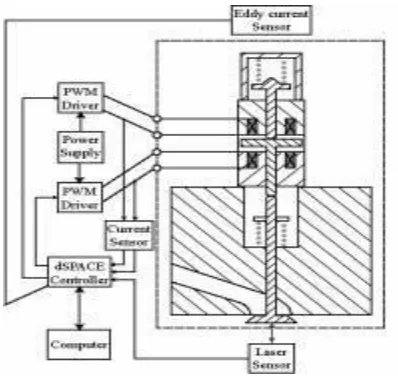
Fig. 9 shows the experimental setup. A 200V prototype actuator is installed on a modified cylinder head and connected to power electronics and a dSPACE rapid control prototyping system. A Power-Ten Model P83 power supply provides the required voltage and current for two Advanced Motion Controls Model 50A-DD pulse-width-modulated (PWM) drivers. These drivers then regulate voltage to the actuator coils. Two LEM HY 15-P sensors are used to measure the coil currents, while a Polytec laser vibrometer is used to measure the position and velocity of the valve. A prototype Eddy current sensor is also used to measure armature position.

The dSPACE system uses a high speed DS1103 controller board to monitor the current, position, and velocity signals, and to send both PWM and voltage polarity control signals to the PWM drivers. For these experiments, the PWM supply voltage is 180V and the PWM frequency is 10 kHz. By controlling the PWM duty cycle and voltage polarity signals, the actuator coil voltages (Vin ) are varied between −180V≤Vin≤180V .

The experimental set-up is used to (i) identify mechanical properties, (ii) perform dynamic measurements to obtain flux linkage characteristics, (iii) validate the model, and (iv) develop control algorithms.

Experimental set-up.

VALVE RELEASING EXPERIMENTS

Fast and accurate valve release is required to accurately control valve timings and ultimately achieve unthrottled load control, good fuel economy and driveability, and low exhaust emissions; therefore, experiments are conducted to study the valve release process. Here, the valve is held in either the open or closed position and then released to freely oscillate on the springs. The delay time between the release command and the beginning of valve motion is measured, and the free oscillation motion is observed.

In initial experiments, voltage polarity control was not implemented and the valve release was commanded by simply setting the PWM apply voltage on the holding coil to V_in0 . A typical result is illustrated in Fig. 10, which shows the current and valve position versus time. The current decays from a holding level of about i ≈0.4 A to about i≈0.1 A, and the valve then begins to move. The long delay time of τ d ≈ 34 ms between the release command and the start of valve motion is consistent with the inductance (L) and resistance (r) of the circuit, which gives a time constant of L/R≈50(mH) / 5(Ω)≈10(ms) . For typical engine speeds (500 RPM < ne < 7000 RPM),

(7)

International Journal of Research (IJR)

Valve release response. The coil apply

voltage is set to Vapp = 0 at time = 14 ms. The

current then decays slowly and valve motion begins at time = 48

ms.

The valve begins moving when the sum of magnetic and frictional forces drops below the spring counter-force. As the valve and armature begin to move, the armature generates an electromotive force (EMF) due to the changing magnetic field passing through the coil windings. This is evident in both Figs. 10 and 11, where the current increases as the valve motion begins. This increase in current increases the magnetic force during the initial motion. This force opposes the valve motion and substantially reduces the kinetic energy and increases transition time. This is shown clearly in Fig. 11, which shows the first oscillation after the valve release, along with an ideal damped oscillation. The opposing magnetic force increases the transition time by about 1-2 ms. Due to the kinetic energy loss, more power must by applied to the opposing coil to catch the valve. These effects should be minimized to improve performance and fuel economy.

Valve release response. Also shown is an ideal

(8)

International Journal of Research (IJR)

CONTROL FOR FAST VALVE RELEASE

Based on the analysis above we need to drive the current on the release coil to zero as fast as possible. We achieve this by applying a reverse polarity voltage pulse with high magnitude of Vin =

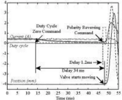
-180V. The duration of the reverse pulse is tuned to cancel the EMF -induced current and allows fast release and travel of the armature. Fig. 12 shows that the delay has been reduced to 1.2 ms and the armature approaches the catching coil faster. This improved travel subsequently requires less power from the catching coil to attract the armature. Additionally, more consistent valve operation can be achieved over a wider range of engine operating conditions.

Voltage polarity control for smaller delay

CONTROL FOR SOFT LANDING

Analysis of the system equations demonstrates that all the equilibria near landing (extreme positions) are unstable. Consider the magnetic and spring force versus air-gap distance diagram shown in Fig. 13.

Figure 13: Magnetic force and spring force versus air-gap distance x between the armature and coil.

The equilibrium position is the point of intersection between the two forces. A perturbation from this equilibrium which decreases x will accelerate the armature towards the coil seat because the magnetic force increases parabolically while the spring force increases linearly. This acceleration can result in high contact velocities if the current is not rapidly adjusted to a lower value. On the other hand, a perturbation which increases x

will reduce the magnetic force and the spring will therefore push the armature towards the middle position. The valve will not be held in the proper position and the engine may not operate correctly. The instability indicates that the system is very sensitive to parameter variations and uncertainties; thus, fast and decisive control action is required.

Unfortunately the interaction between the electromagnetic and mechanical subsystems is limited. When the distance is more than 1 mm, the magnetic force is relatively small and has little effect on the armature position. The armature motion is mostly determined by the mechanical spring, damping, and gas disturbance forces. Thus, the controller output voltage is only effective during the last 10% of the travel. Moreover, the electromagnetic system, which controls the current and the magnetic force on the armature, has a time constant of the same order as the valve transition time.

To summarize, soft landing is fundamentally difficult to achieve because the system is (i) highly nonlinear, (ii) unstable and has low control authority, and (iii) uncertain with varying parameters and fast disturbances.

OPEN LOOP CONTROL

Using the nonlinear model in Eq. 11 we investigate the effects of the control variables,

(9)

International Journal of Research (IJR)

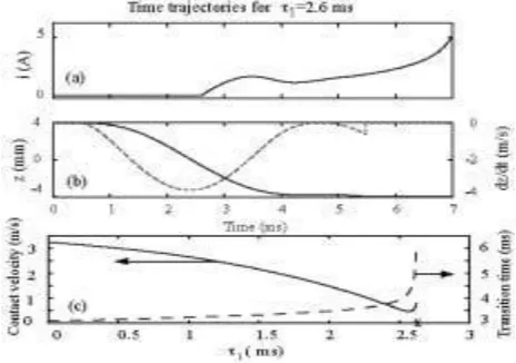
the time interval between the valve motionand holding

voltage application. Fig. 14c shows that increasing τ₁

will decrease contact velocity while increasing travel

time. Simulation results also show that when τ₁ is too

large, catching cannot be achieved. Moreover, for a

small range of τ₁ values, both the contact velocity and

transition time increase. This happens because a counter-EMF is induced when the armature approaches the coil. This reduces the current, and the magnetic force falls below the spring counter-force. The armature then begins to move away, and this reverses the polarity of the induced EMF. The current then increases (Fig. 14a), and a stronger magnetic force pulls the armature back into the coil with high impact velocity (Fig. 14b).

Similar results are observed for varying τ2 , and dc . Fig. 15 summarizes the model predictions as a cross plot of contact velocity versus transition time. It also shows measured closed-loop results that will be discussed later. The model results demonstrate that, for a simple open-loop control scheme (varying τ₁ , τ

2 , and dc ), minimizing the contact velocity increases the transition time. Of course, the voltage command sequence used here is not optimal, but this simple control scheme is clearly limited because the results for contact velocity and transition time fall outside of the desired range. Similar behavior with "one-step-change" current trajectory has also been presented in [1]. One can allow the voltage to switch on and off following an optimal pattern. The optimal number of switches can be determined numerically using a model and optimization techniques similar to the ones in [4].

Contact velocity and travel time versus τ1

Contact velocity versus travel time by varying a one- step-change in voltage command. Comparison results with the feedback control are discussed later.

A smooth voltage trajectory (infinitely many switches) can potentially achieve better results. A feedback control algorithm may give a better voltage command trajectory. This trajectory can then be used for open-loop operation.

LEARNING FEEDFORWARD CONTROL

A smooth voltage trajectory u* can be pre-calculated by inverting the model equations in Eq. 11 to satisfy desired valve position zdes(t) and velocity vdes(t) trajectories. This task can be simplified if we assume that Fgas 0 , and that the desired motion is undamped and harmonic.

Note here that

i

des

(

t

)

can be calculated based on

z des(t)and v des(t). For a simplified algebraic solution of the u* based on [i(t),z(t),v(t)]des , we neglect the saturation region of the magnetic subsystem.

The resulting control signal u* will not exactly achieve the desired position and velocity trajectories; however, u*can be enhanced with

a closed loop control signal u_cl for better

performance.

(10)

International Journal of Research (IJR)

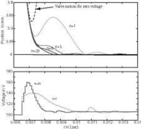
only for very long transitions (10 ms). The authors in [1] do not specify which error they used in their cycle adaptation. Finally, the authors in [5] use the error in momentum at the middle position only. In general, one-point adaptation entails high sensitivity and poor repeatability due to combustion and noise. We adjust our feedforward control signal based on the weighted error between the desired and the actual valve position, which is sampled about 20 times during the last 1.0 mm of the valve transition [3]. The weights are selected to achieve fast cycle-to-cycle learning, and to converge to the optimum feedforward control signal without the large corrections that may degrade repeatability [2]. Fig. 16 shows simulations of the cycle-to-cycle adjustments using the feedforward iterative learning controller. The learning algorithm converges towards the desired trajectory.

Positions z, zdes and lower voltage Vlfor cycles k∈

[1,3,5,20] .

POSITION FEEDBACK CONTROL

Designing a feedback controller is a challenging task. The system is unstable near landing, and thus requires a high bandwidth controller to achieve the stabilization and performance objectives (travel time of 3-4 ms). Unfortunately, the time constant of the electrical subsystem, which controls the current and the magnetic force on the armature, is in the range of several ms. As a result, there are severe bandwidth limitations and control difficulties.

To overcome the slow dynamics of the magnetic coils, it is necessary to anticipate fast transients

while the armature is far from landing. A closed loop controller using this scheme may give large voltage commands and saturate since the electromagnetic force is weak at large distances. The application of a preset [3] or a cycle-to-cycle varying [2] open loop voltage at large distances may be followed by closed loop control at small distances; however, this may not be a robust solution. Improved performance can be achieved by using a carefully tuned controller that penalizes deviations from the nominal catching current much more than deviations in position or velocity when the armature is far away. We use a linear approximation of the system in Eq. 11 and linear quadratic optimization to tune three static controller gains. These gains are chosen so that, in the far-away region, the control voltage is based primarily on errors in current, and secondarily on errors in position, and velocity. When the armature is near the contact position, the controller then switches to a second set of feedback gains that are chosen to ensure soft landing of the valve by penalizing errors in position and velocity.

The two distinct stages of the controller are evident in Fig. 17, which shows position, current, velocity, and voltage for a typical closed-loop experiment. The voltage first increases to about 100V and then drops to about 25V as the armature travels through the far region. Then, when the controller switches to the near region gains, the voltage first increases rapidly and then drops off as the armature lands. With this more optimal voltage trajectory, the impact velocity is 0.16 m/s and the travel time is 3.42 ms. Table 1 shows statistics from 50 runs.

Transition Time Contact Velocity Mean 3.42 ms 0.16 m/s

σ .02 ms 0.09 m/s Max 4.3 ms 0.35 m/s Min 3.3 ms 0.06 m/s Table 1: Transition time and contact

velocity results of closed-loop experiment. 50 data points.

(11)

International Journal of Research (IJR)

velocity and current are achieved using a nonlinear observer. High accuracy and speed of response are obtained by combining a copy of the identified nonlinear system dynamics in Eq. 11 with a linear correction of the error between the estimated and the actual position signal. We analyzed the system and eliminated its weakly observable states, and then tuned the gains for the linear correction term for fast convergence. Fig. 18 shows reasonable agreement between the measured and estimated states.

parameter variations; experimental results are left for future work.

Although the experimental results presented are close to the desired operating requirements, more development is required to further reduce contact velocities and improve repeatability. In the future we plan to include the valve lash and

use a 42 Volt actuation system An average soft

landing achieved by the observer based output feedback controller.

Comparison of the actual states versus the estimated states from the nonlinear observer.

CONCLUSIONS

An EMV actuator model was developed and experiments were used to identify unknown model parameters and functions and to validate the model predictions.

An open loop controller that reduced the valve motion delay in the releasing phase from 34 ms to 1.2 ms was designed and implemented.

A position feedback closed-loop controller that reduced the valve landing velocity from 0.55 m/s to 0.16 m/s with consistent transition time of 3.42 ms was designed and implemented.

Simulation results indicate that, by applying an

iterative learning algorithm, the valve

(12)

International Journal of Research (IJR)

REFERENCES

[1] S. Butzmann, J. Melbert, A. Koch, "Sensorless Control of Electromagnetic Actuator for Variable Valve Train", SAE Paper No. 2000-01-1225, 2000.

[2] W. Hoffmann and A. G. Stefanopoulou, "Iterative Learning Control of Electromechanical Camless Valve Actuator", Proceedings American Control Conference, pp. 2860-2866, June 2001.

[3] W. Hofmmann and A. G. Stefanopoulou, Valve Position Tracking for Soft Landing of Electromechanical Camless Valvetrain", Proceedings IFAC workshop on Automotive Control, pp. 305-310, Kalsruhe, March 2001. [4] I. V. Kolmanovsky, A. G. Stefanopoulou, "Evaluation of Turbocharger Power Assist System Using Optimal Control Techniques", SAE 2000-01-0519, SAE World Congress, March 2000.

[5] V. F. Schultz, and W. E. Seitz, "Gently Does It", press release of Venture Scientifics, LLC, 1997.

[6] C. Tai, A. Stubbs, and T.C. Tsao, "Modeling and Controller Design of an Electromagnetic Engine Valve", Proceedings of American Control Conference, pp. 2890-2895, June 2001.

[7] Y. Wang, A. Stefanopoulou, M. Haghgooie, I. Kolmanovsky, and M. Hammoud, "Modeling of an Electromechanical Valve Actuator for a Camless