Removal of Artifacts Based on Weighted Guided Image Filtering For Improving Visual Quality of an Image

(1)

Available online: http://edupediapublications.org/journals/index.php/ijr P a g e | 124

Removal of Artifacts Based on Weighted Guided Image Filtering For

Improving Visual Quality of an Image

Dr. Y. Raghavender Rao (Associative Prof., M,E, MISTE, Ph.D)

1

Chirupaka Anjaneyulu

(M .tech ) 2

1_{JNTUH Co lleg e o f En g in eerin g , Jag itial, Nach u p ally , Karimn ag ar, TS-505501, INDIA}

2_{JNTUH Co lleg e o f En g in eerin g , Jag itial, Nach u p ally , Karimn ag ar, TS-505501, INDIA}

1

_{y rag h av en d errao @g mail.co m}

2 1_{an jich iru p aka@g mail.co m}

A b s tract

In this paper, a weighted guided image filter (WGIF) is proposed to address the problems faced by the existing methods such as global and local filtering techniques. Local filtering-based edge preserving smoothing techniques suffer from halo artifacts. The global optimization based filters often yield excellent quality, they have high computational cost. The WGIF receives advantages of both global and local smoothing filters in the sense that: 1) the complexity of the WGIF is O(N) for an image with N pixels, which is same as the GIF and 2) the WGIF can avoid halo artifacts like the existing global smoothing filters. The WGIF is applied for single image detail enhancement, single image haze removal, and fusion of differently exposed images. Experimental results shows that the resultant image produces better visual quality by reducing/avoiding the halo artifacts to zero.

KEYW ORDS: Edge-preserving smoothing, weighted guided image filter, edge aware weighting, detail enhancement, haze removal, exposure fusion

1. INTRODUCTION

(2)

Halo artifacts were usually produced by the local filters when they were adopted to smooth edges. Major reason that the BF/GIF produces halo artifacts was both spatial similarity parameter and range similarity parameter in the BF were fixed. But both the spatial similarity and the range similarity parameters of the BF could be adaptive to the content of the image to be filtered. Unfortunately as pointed out, problem with adaptation of the parameters will destroy the 3D convolution form. We introduce in present paper, an edge-aware weighting technique and incorporated into the GIF to form a weighted GIF (WGIF). Local variance in 3×3 window of pixel in a guidance image is applied to calculate the edge-aware weighting. The local variance of a pixel is normalized by the local variance of all pixels in guidance image. The normalized weighting is then adopted to design the WGIF. As a result, halo artifacts can be avoided by using the WGIF. Similar to the GIF, the WGIF also avoids gradient reversal. In addition, the intricacy of the WGIF is O(N) for an image with N pixels which is the same as that of the GIF. These features allow many applications of the WGIF for single image detail enhancement, single image mist removal, and fusion of differently exposed images.

2. EDGE PRESERVING SMOOTHING

TECHNIQUES

The task of edge-preserving smoothing is to crumble an image X into two parts as follows:

X (p) = 𝑗̂(p) +r (p)

where Ĵ is a reconstructed image formed by uniform regions with sharp edges, e is noise or texture, and p(=(x,y)) is a position. Ĵ and e are called base layer and detail layer, respectively. One of edge-preserving

smoothing techniques is based on local filtering. Bilateral filter( BF) is widely used due to its simplicity but suffer from “gradient reversal” artifacts usually observed in detail enhancement of conventional LDR images. Then GIF was introduced to overcome this problem. In this GIF, a guidance image G was used which could be similar to the image X which is to be filtered.

Ĵ is a linear transform of G in the window Ως (pʹ ).To determine the linear coefficients (apʹ , bpʹ ), a constraint is added to X and Ĵ as in Equation (1). The values of apʹ and bpʹ are then obtained by minimizing a cost function E (apʹ ,bpʹ ) which is defined as

𝐸 = ∑ [(𝑎𝑝′𝐺(𝑝) + 𝑏𝑝′− 𝑋(𝑝))2 𝑃€Ω𝜍

+ 𝜆𝑎𝑝′2] (2)

where λ is a regularization parameter.

Another type of edge-preserving smoothing techniques was based on global optimization. The Weighted Least Square filter was a typical example and it was derived by minimizing the following quadratic cost function:

𝐸 = ∑ [(𝑗̂(𝑝) − 𝑋(𝑝))2_{+ 𝜆(𝑝)‖∇𝑗̂(𝑝)‖}2_{] (3)} 𝑁

𝑃 =1

where N is the total number of pixels in an image. The two major differences between the WLS filter and the GIF

(3)

2) The value of λ is fixed in the GIF while it is adaptive to local gradients in the WLS filter. One possible problem for the GIF is halos which could be reduced by the WLS filter. The spatial varying image gradients aware weighting λx(p)and λy(p) are very important for the WLS filter to avoid halo artifacts.

Figure 1(a): Input image

Figure 1(b): Edge of input image

3. EXISTING METHODS

a) Bilateral Filter

The bilateral filter was perhaps the simplest which computed the filtering output at each pixel as the average of near-by pixels, weighted by the Gaussian of both range and spatial distance. The bilateral filter smooth’s the image while preserving edges. Constraint of the bilateral filter was it endure from “gradient reversal” artifacts. The reason was that when a pixel (often on an edge) has few similar pixels around it, the Gaussian weighted average is unstable. Efficiency was another problem regarding the bilateral filter.

b ) No n -av erag e Filter

Edge-preserving filtering could also be achieved by non average filters. The median filter was a familiar edge-aware operator, and was a special case of local histogram filters. Histogram filters had O(N) time implementations in a way as the bilateral grid. The non-average filters were often computationally expensive.

c) Gu id ed Imag e Filter

A general linear translation-variant filtering process, which involved a guidance image I, an filtering input image p, and an output image q. The filtering output at a pixel I was expressed as a weighted average:

𝑞𝑖 = ∑ 𝑊𝑖𝑗(𝐼)𝑝𝑗𝑗 (4)

(4)

d ) A d ap tiv e Bilateral Filter

Both range similarity parameter and spatial similarity parameter were adaptive to the content of filtered image. However, adaptation of the parameters destroyed the 3-D convolution form. It was time consuming to extract fine details from a set of differently exposed images by the content adaptive bilateral filters because each input image needed to be decomposed individually. A content adaptive bilateral filter was proposed in gradient domain by taking the characteristics of the human visual systems into consideration.

e) Adaptive Guided Image Filter

An adaptive guided image filtering (AGF) able to perform halo-free edge slope enhancement and noise reduction simultaneously. The intensity range domain of BLF and kernel function of GIF were similar in principle, because each of them takes the intensity value of center pixel p, local neighbors q and a smoothing parameter (σr in BLF, ε in GIF) in the computation process. This was based on the shifting technique of ABF, in which the offset ξp was added to the intensity value of center pixel pin the intensity range domain of BLF. The same strategy was applied to AGF - the offset is added to the intensity value of center pixel pin the kernel weights function of GIF.

4. PROPOSED METHOD

In this, an edge-aware weighting is first proposed and it is incorporated into the GIF to form the WGIF.

A ) A n Ed g e -A ware W eig h tin g

Let G be a guidance image and be the variance of G in the 3 × 3 window,. An edge-aware weighting is

defined by using local variances of 3 × 3 windows of all pixels as follows

Γ_𝐺(𝑝′₎= 1

𝑁∑

𝜎𝐺 ,12 (𝑝′) + 𝜀

𝜎𝐺,12 (𝑝) + 𝜀

𝑁

𝑝=1

(5)

Where ε is a small constant and its value is selected while L is the dynamic range of the input image.

In addition, the weightingΓ𝐺(𝑝′) measures the

importance of pixel 𝑝′ with respect to the whole guidance image. Due to the box filter, the complexity

ofΓ𝐺(𝑝′)is O (N) for an image with N pixels. The

value of Γ𝐺(𝑝′) is usually larger than 1 if 𝑝′ is at an

edge and smaller than 1 if 𝑝′ is in a smooth area. Clearly, larger weights are assigned to pixels at edges than those pixels in flat areas by using the weight

Γ𝐺(𝑝′) in Equation (5).

B) Th e Pro p o s ed Filter

Same as the GIF, the key assumption of the WGIF is a local linear model between the guidance

image G and the filtering output 𝑍̂as in Equation (2).

The model ensures that the output 𝑍̂ has an edge only if the guidance image G has an edge. The proposed weighting G( p) in Equation (5) is incorporated into the cost function E(a p, b p) in Equation (3). As such, the solution is obtained by minimizing the difference between the image to be filtered X and the filtering

output𝑍̂ while maintaining the linear model (2), i.e., by minimizing a cost function E(𝑎_𝑝′, 𝑏_𝑝′)which is

defined as

E = ∑ [(𝑎𝑝′𝐺(𝑝) + 𝑏𝑝′− 𝑋(𝑝)) 2

+ 𝜆

Γ_𝐺(𝑝′₎𝑎𝑝′ 2_]

𝑝𝜖Ω_𝜁1( 𝑝′) (6)

The optimal values of 𝑎_𝑝′ and 𝑏_𝑝′ are computed as

𝑎_𝑝′ =

𝜇𝐺⨀𝑋,𝜁1(𝑝′) − 𝜇𝐺,𝜁1(𝑝′)𝜇𝑋,𝜁1(𝑝′)

𝜎_𝐺,𝜁2 ₁_(𝑝′_{) +} 𝜆 Γ𝐺 (𝑝′)

(7)

(5)

where ⨀ is the element-by-element product of two matrices. 𝜇𝐺⨀𝑋,𝜁1(𝑝

′_{), 𝜇}

𝐺,𝜁1(𝑝

′₎_and_𝜇

𝑋,𝜁1(𝑝

′₎_{are the}

mean values of G ⨀ X, G and X, respectively. The final value of Zˆ ( p) is given as follows:

𝑍̂(𝑝) = 𝑎̅𝑝𝐺(𝑝) + 𝑏̅𝑝 (9)

Where 𝑎̅𝑝 and 𝑏̅𝑝 are the mean values of and in

the window computed as

𝑎̅𝑝= 1

|Ω_𝜁1(𝑝) | ∑𝑝′𝜖Ω𝜁1(𝑝)𝑎𝑝′ ; 𝑏̅𝑝= 1

|Ω_𝜁1(𝑝) | ∑𝑝′𝜖Ω𝜁1(𝑝)𝑏𝑝′ (10)

And |Ω_𝜁₁(𝑝′_)|_{is the cardinality of}_Ω

𝜁1(𝑝

′₎_.

C.

Single Image Haze Removal

Images of outdoor scenes could be degraded by haze, fog, and smoke in the atmosphere. The degraded images lose the contrast and color fidelity. Haze removal is thus highly desired in both computational photography and computer vision applications. The model adopted to describe the formulation of a haze image is given as

𝑋𝑐(𝑝) = 𝑍̂𝑐(𝑝)𝑡(𝑝) + 𝐴𝑐(1 − 𝑡(𝑝) ) (10)

When the atmosphere is homogenous, the transmission t( p) can be expressed as:

𝑡(𝑝) = 𝑒−𝑎𝑑(𝑝)₍₁₁₎

Let 𝜙𝑐(∙) be a minimal operation along the color

channel {r, g, b} and it is defined as

Amin = ϕc(Ac) = min{Ar, Ag, Ab} (12)

Xmin(p) = ϕc(Xc(p))

= min{Xr(p) ,Xg(p) , Xb(p)} (13)

Ẑmin(p) = ϕc(Ẑ c(p))

= min{Ẑr(p) , Ẑg(p), Ẑb(p)} (14)

it can be derived from the haze image model in Equation (15) that

𝑋𝑚𝑖𝑛(𝑝) = 𝑍̂𝑚𝑖𝑛(𝑝) 𝑡(𝑝)

+ 𝐴𝑚𝑖𝑛(1 − 𝑡(𝑝) ) (15)

Let 𝜓𝜁2(∙)be a minimal operation in the

neighborhood 𝜓𝜁2(𝑝)and it is defined as

𝜓𝜁2(𝑧(𝑝) ) = min_𝑝′_𝜖_Ω

𝜁2(𝑝)

{𝑧(𝑝′_{)} (16)}

It is shown that the complexity of 𝜓𝜁2(∙) is O(N)

for an image with N pixels. The dark channel is defined as

𝐽𝑑𝑎𝑟𝑘𝑍̂ (𝑝)=𝜙𝑐(𝜓𝜁2(𝑍̂𝑐(𝑝))) (17)

where the value of 𝜁2 is 7. Even though the

complexity of 𝜓𝜁2(∙) is O(N) for an image with N

pixels, three minimal operations 𝜓𝜁2(∙)and one

minimal operation Φ𝑐(∙)are required to compute

𝐽𝑑𝑎𝑟𝑘𝑍̂ (𝑝) for the pixel p. simplified dark channel is

defined as

𝐽̂𝑑𝑎𝑟𝑘𝑍̂ (𝑝) = 𝜓𝜁2(𝜙𝑐(𝑍̂𝑐(𝑝))) (18)

The value of 𝑡(𝑝) is assumed to be constant in the

neighborhood Ω𝜁1(𝑝

′₎_{. It can be derived from}

Equation (20) that

𝐽̂𝑑𝑎𝑟𝑘𝑋 (𝑝) = 𝐽̂𝑑𝑎𝑟𝑘𝑍̂ (𝑝) 𝑡(𝑝)

+ 𝐴𝑚𝑖𝑛(1 − 𝑡(𝑝) ) (19)

Since 𝐽̂𝑑𝑎𝑟𝑘𝑍̂ (𝑝) ≈ 0, the value of 𝑡(𝑝) can be initially

estimated as

𝑡(𝑝) = 1 −𝐽̂𝑑𝑎𝑟𝑘

𝑋 _(𝑝)

𝐴𝑚𝑖𝑛

(20)

It is worth noting that the initial value of t( p) is given as

𝑡(𝑝) = 1 − 𝜙𝑐( 𝜓𝜁₂(

𝑍̂𝑐(𝑝)

𝐴𝑐

)) (21)

The initial value of 𝑡(𝑝)is then computed as

𝑡(𝑝) = 1 −31 32

𝐽̂𝑑𝑎𝑟𝑘𝑋 (𝑝)

𝐴𝑚𝑖𝑛

(6)

The value of λ is set to 1/1000 and the value of 𝜁1 to

60. The value of the transmission map 𝑡(𝑝) is further adjusted as

𝑡(𝑝) = 𝑡1+𝜍(𝑝) (23)

where the value of 𝜍 is adaptive to the haze level of the input image. Its value is 0/0.03125/0.0625 if the input image is with light/normal/heavy haze.

Finally, the scene radiance 𝑍̂(𝑝) is recovered by

𝑍̂𝑐(𝑝) =

𝑋𝑐(𝑝)−𝐴𝑐

𝑡(𝑝) +𝐴𝑐 ;c 𝜖{𝑟, 𝑔, 𝑏} (24)

Equation (29) is equivalent to

𝑍̂𝑐(𝑝) = 𝑋𝑐(𝑝)

+ ( 1

𝑡(𝑝)− 1) (𝑋𝑐(𝑝)

− 𝐴𝑐) (25)

Since the color of the sky is usually very similar to the atmospheric light Ac in a haze image, it can be shown that

𝐽̂𝑑𝑎𝑟𝑘𝑋 (𝑝)

𝐴𝑚𝑖𝑛

→ 1, 𝑎𝑛𝑑 , 1

𝑡(𝑝)− 1 → 31 (26)

D. Fu s io n o f Differen tly Exp o s ed Imag es One of the challenges in digital image processing research is the rendering of a HDR natural scene on a conventional LDR display. This challenge can be addressed by capturing multiple LDR images at different exposure levels. Each LDR image only records a small portion of the dynamic range and partial scene details but the whole set of LDR images collectively contain all scene details . All the differently exposed images can be fused together to produce a LDR image by an exposure fusion algorithm. Similar to the detail enhancement of a LDR image, halo artifacts, gradient reversal artifacts and amplification of noise in smooth regions are

three major problems to be addressed for the fusion of differently exposed images.

5. SIMULATION RESULTS

Figure 2: (a) Input image (b) Guided image (c) Enhanced image by GIF (d) Enhanced image by WGIF

Analysis 2: In the above figure first is the input image which is to be analyzed and the second is guided image which is not but a filtering technique which preserves the edges of an image, the third one is GIF image with less preserving edges. The last one is proposed method which shows image with zero artifacts.

Figure 3: Weighted image

(7)

Figure 4: (a) Input image (b) Guided image (c) Dehazed image by GIF (d) Dehazed image by WGIF Analysis 4: The above figure is used to dehaze the image from smoke etc as shown by applying different techniques.

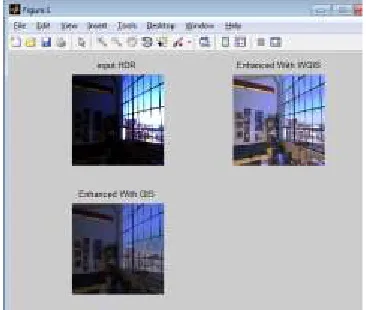
Figure 5: (a) Input HDR (b) Enhanced with WGIS (c) Enhanced with GIS

Analysis 5: This figure is used to show the enhancement of an image with improved picture quality by different edge preserving techniques .

6. EXTENSION

Proposed method has been performed improved image quality on images. For extension, we are performing on videos. Compare to images the complexity for videos is more because a video consist of no. of frames. As the no. of frames

increases the reduction of complexity is also gets increased. But, avoiding all these complexities every frame is avoiding halo artifacts and preserves edges. At last all these frames converted into video.

Figure 6: Input video

Analysis 6: The above figure shows the input video which consist of some set of frames.

Figure 7: GI Video

(8)

Figure 8: GIF Video

Analysis 8: The above figure shows GIF video which has better quality than the GI video .

Figure 9: WGIF Video

Analysis 9: The above figure shows WGIF video which has better image quality than the GIF video .

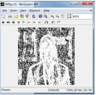
Figure 10: Weights on WGIF Video

Analysis 10: The above figure shows weights applied on WGIF video to preserves edges.

7. CONCLUSION

This method is introduced by incorporating an edge-aware weighted into an existing guided image filter (GIF). It has two advantages of both global and local smoothening filter in the sense-(1) Its complexity is 0,(2)Avoid halo artifacts The output of WGIF results in better visual quality and avoid halo artifacts. , it has many applications in the fields of computational photography and image processing. Particularly, it is applied to study single image detail enhancement, single image haze removal, and fusion of differently exposed images. Experimental results show that the esultant algorithms can produce images with excellent visual quality as those of global filters, and at the same time the running times of the proposed algorithms are comparable to the GIF based algorithms. It is noting that the WGIF can also be adopted to design a fast local tone mapping algorithm for high dynamic range images, joint up sampling, flash/no-flash de-noising, and etc. In addition, similar idea can be used to improve the anisotropic diffusion, Poisson image editing, etc. All these research problems will be studied in our future research.

REFERENCES

(9)

[3] Z. G. Li, J. H. Zheng, and S. Rahardja, “Detail-enhanced exposure fusion,” IEEE Trans. Image Process., vol. 21, no. 11, pp. 4672–4676, Nov. 2012. [4] Z. Farbman, R. Fattal, D. Lischinski, and R. Szeliski, “Edge-preserving decompositions for multi-scale tone and detail manipulation,” ACM Trans. Graph., vol. 27, no. 3, pp. 249–256, Aug. 2008. [5] R. Fattal, M. Agrawala, and S. Rusinkiewicz, “Multiscale shape and detail enhancement from multi-light image collections,” ACM Trans. Graph., vol. 26, no. 3, pp. 51:1–51:10, Aug. 2007.

[6] P. Pérez, M. Gangnet, and A. Blake, “Poisson image editing,” ACM Trans. Graph., vol. 22, no. 3, pp. 313–318, Aug. 2003.

[7] K. He, J. Sun, and X. Tang, “Single image haze removal using dark channel prior,” IEEE Trans. Pattern Anal. Mach. Intell., vol. 33, no. 12, pp. 2341– 2353, Dec. 2011.

[8] L. Xu, C. W. Lu, Y. Xu, and J. Jia, “Image smoothing via L0 gradient minimization,” ACM Trans. Graph., vol. 30, no. 6, Dec. 2011, Art. ID 174. [9] C. Tomasi and R. Manduchi, “Bilateral filtering for gray and color images,” in Proc. IEEE Int. Conf. Comput. Vis., Jan. 1998, pp. 836–846.

[10] Z. Li, J. Zheng, Z. Zhu, S. Wu, and S. Rahardja, “A bilateral filter in gradient domain,” in Proc. Int. Conf. Acoust., Speech Signal Process., Mar. 2012, pp. 1113–1116.

[11] P. Choudhury and J. Tumblin, “The trilateral filter for high contrast images and meshes,” in Proc. Eurograph. Symp. Rendering, pp. 186–196, 2003. [12] F. Durand and J. Dorsey, “Fast bilateral filtering for the display of highdynamic-range images,” ACM Trans. Graph., vol. 21, no. 3, pp. 257–266, Aug. 2002.

[13] J. Chen, S. Paris, and F. Durand, “Real-time edge-aware image processing with the bilateral grid,” ACM Trans. Graph., vol. 26, no. 3, pp. 103–111, Aug. 2007.

[14] K. He, J. Sun, and X. Tang, “Guided image filtering,” IEEE Trans. Pattern Anal. Mach. Intell., vol. 35, no. 6, pp. 1397–1409, Jun. 2013.