Combined Economic Emission Dispatch
Solution using Modified Artificial Bee Colony
Algorithm
Hardiansyah
1, Rusman
2Dept. of Electrical Engineering, University of Tanjungpura, Indonesia1
Dept. of Electrical Engineering, State Polytechnic of Pontianak, Indonesia 2
ABSTRACT: In this paper, a new approach is proposed to solve combined economic emission dispatch (CEED) problem in power systems using modified artificial bee colony (MABC) algorithm considering the power limits. The CEED is to minimize both the operating fuel cost and emission level simultaneously while satisfying the load demand and operational constraints. A novel best mechanism algorithm based on ABC algorithm, in which a new mutation strategy inspired from the differential evolution (DE) is introduced in order to improve the exploitation process. The effectiveness of the proposed algorithm has been tested on IEEE 30-bus test system and the results were compared with other methods reported in recent literature. The simulation results show that the proposed algorithm outperforms previous optimization methods.
KEYWORDS: Economic dispatch, emission dispatch, combined economic emission dispatch, modified artificial bee colony algorithm, differential evolution.
I. INTRODUCTION
Economic dispatch (ED) is one of the most fundamental issues in power system operation and control for allocating generation among the committed units. The objective of the ED problem is to determine the amount of real power contributed by online thermal generators satisfying load demand at any time subject to unit and system constraints so as the total generation cost is minimized. Therefore, it is very important to solve the problem as quickly and precisely as possible [1, 2]. Therefore, recently most of the researchers made studies for finding the most suitable power values produced by the generators depending on fuel costs. In these studies, they produced successful results by using various optimization algorithms [3-5]. Despite the fact that the traditional ED can optimize generator fuel costs, it still can not produce a solution for environmental pollution due to the excessive emission of fossil fuels.
Currently, a large part of energy production is done with thermal sources. Thermal power plant is one of the most
important sources of carbon dioxide (CO2), sulfur dioxide (SO2) and nitrogen oxides (NOx) which create atmospheric
pollution [6]. Emission control has received increasing attention owing to increased concern over environmental pollution caused by fossil based generating units and the enforcement of environmental regulations in recent years [7]. Numerous studies have emphasized the importance of controlling pollution in electrical power systems [8].
Combined economic and emission dispatch (CEED) has been proposed in the field of power generation dispatch, which simultaneously minimizes both fuel cost and pollutant emissions. When the emission is minimized the fuel cost may be unacceptably high or when the fuel cost is minimized the emission may be high. A number of methods have been presented to solve CEED problems such as simplified recursive method [9], genetic algorithm [10-12], simulated annealing [13], biogeography based optimization [14], particle swarm optimization [15, 16], and artificial bee colony algorithm [17, 18].
called MABC is proposed. Combined economic emission dispatch (CEED) solution which was performed using MABC algorithm was tested over a standard IEEE 30-bus test system which consisted of six generators. The results were compared to those reported in the literature.
II. PROBLEM FORMULATIONS
The EED problem targets to find the optimal combination of load dispatch of generating units and minimizes both fuel cost and emission while satisfying the total power demand. Therefore, EED consists of two objective functions, which are economic and emission dispatches. Then these two functions are combined to solve the problem. The EED problem can be formulated as follows [11]:
F
T
Min
f
FC
,
EC
(1)where FT is the total generation cost of the system, FC is the total fuel cost of generators and EC is the total emission of
generators.
2.1 Economic Dispatch (ED)
The ED problem targets to find the optimal combination of power generation by minimizing the total fuel cost of all generator units while satisfying the total demand. The ED problem can be formulated in a quadratic form as follows [11]:
N i i i i i iC
a
P
b
P
c
F
1 2
(2)
where Pi is the power generation of the ithunit; ai, bi, and ci are fuel cost coefficients of the i th generating unit and N is
the number of generating units.
2.2 Emission Dispatch (ED)
The classical ED problem can be obtained by the amount of active power to be generated by the generating units at minimum fuel cost, but it is not considered as the amount of emissions released from the burning of fossil fuels. Total amount of emissions such as SO2 or NOx depends on the amount of power generated by until and it can be defined as the sum of a quadratic function as follows [11]:
N i i i i ii
P
P
EC
1
2
(3)where αi,βi and γi are emission coefficients of the ith generating unit.
2.3 Combined Economic Emission Dispatch (CEED)
CEED is a multi-objective problem, which is a combination of both economic and environmental dispatches that individually make up different single problems. At this point, this multi-objective problem needs to be converted into single-objective form in order to fulfill optimization. The conversion process can be done by using the price penalty factor. However, the single-objective EED can be formulated as shown in equation (4) [11, 18]:
($
/
)
1 2 2h
P
P
h
c
P
b
P
a
F
Min
N i i i i i i i i i i i i T
(4)where hi is the price penalty factor, and is formulated as follows:
i i i i i i i i i i i
P
P
c
P
b
P
a
h
max 2 max max 2max (5)
where Pi max is the maximum power generation of the ith unit in MW.
2.4 Problem Constraints
Power balance constraint:
D L
N
i
i
P
P
P
1
(6)
N
i N
j
j i ij
L
B
P
P
P
(7)Generating capacity constraint:
P
im in
P
i
P
im ax (8)where PD is total demand of the system (MW), and PL is total power loss (MW). Pimin, Pimax, and Bij are minimum
generation of unit i (MW), maximum generation of unit i (MW), and coefficients of transmission losses respectively.
III. ARTIFICIAL BEE COLONY (ABC) ALGORITHM
Artificial bee colony is one of the most recently defined algorithms by Karaboga in 2005, motivated by the intelligent behaviour of honey bees [19, 20]. In the ABC system, artificial bees fly around in the search space, and some (employed and onlooker bees) choose food sources depending on the experience of themselves and their nest mates, and adjust their positions. Some (scouts) fly and choose the food sources randomly without using experience. If the nectar amount of a new source is higher than that of the previous one in their memory, they memorize the new position and forget the previous one [20]. Thus, the ABC system combines local search methods, carried out by employed and onlooker bees, with global search methods, managed by onlookers and scouts, attempting to balance exploration and exploitation process.
In the ABC algorithm, the colony of artificial bees consists of three groups of bees: employed bees, onlooker bees, and scout bees. The main steps of the ABC algorithm are described as follows:
• Initialize. • REPEAT.
(a) Place the employed bees on the food sources in the memory; (b) Place the onlooker bees on the food sources in the memory;
(c) Send the scouts to the search area for discovering new food sources; (d) Memorize the best food source found so far.
• UNTIL (requirements are met).
In the ABC algorithm, each cycle of the search consists of three steps: moving the employed and onlooker bees onto the food sources, calculating their nectar amounts respectively, and then determining the scout bees and moving them randomly onto the possible food source. Here, a food source stands for a potential solution of the problem to be optimized. The ABC algorithm is an iterative algorithm, starting by associating all employed bees with randomly
generated food solutions. The initial population of solutions is filled with SN number of randomly generated D
dimensions. Let Xi= {xi1, xi2, …, xiD} represent the ith food source in the population, SN is the number of food source
equal to the number of the employed bees and onlooker bees. D is the number of optimization parameters. Each
employed bee xijgenerates a new food source vij in the neighborhood of its currently associated food source by (9), and
computes the nectar amount of this new food source as follows:
v
ij
x
ij
ij
x
ij
x
kj
(9)where
ij
(
rand
0
.
5
)
2
is a uniformly distributed real random number within the range [-1, 1],
SN
i
1
,
2
,
,
,k
int(
rand
SN
)
1
andk
i
, andj
1
,
2
,
,
D
are randomly chosen indexes. Thenew solution viwill be accepted as a new basic solution, if the objective fitness of viis smaller than the fitness of xi,
otherwise xi would be obtained.
;
1
)
max(
i i i
fit
fit
p
(10)where fitiis the fitness value of the solution i evaluated by its employed bee. Obviously, when the maximum value of
the food source decreases, the probability with the preferred source of an onlooker bee decreases proportionally. Then the onlooker bee produces a new source according to (9). The new source will be evaluated and compared with the primary food solution, and it will be accepted if it has a better nectar amount than the primary food solution.
After all onlookers have finished this process, sources are checked to determine whether they are to be abandoned. If the food source does not improve after a determined number of the trails “limit”, the food source is abandoned. Its employed bee will become a scout and then will search for a food source randomly as follows:
x
ij
x
jm in
rand
(
0
,
1
)
x
jm ax
x
jm in
(11)where xj min and xj maxare lower and upper bounds for the dimension j respectively.
After the new source is produced, another iteration of the ABC algorithm will begin. The whole process repeats again till the termination condition is met.
IV. MODIFIED ARTIFICIAL BEE COLONY (MABC) ALGORITHM
Following this spirit, a modified ABC algorithm inspired from differential evolution (DE) to optimize the objective function of the ED problems. Differential evolution is an evolutionary algorithm first introduced by Storn and Price [23, 24]. Similar to other evolutionary algorithms, particularly genetic algorithm, DE uses some evolutionary operators like selection recombination and mutation operators. Different from genetic algorithm, DE uses distance and direction information from the current population to guide the search process. The crucial idea behind DE is a scheme for producing trial vectors according to the manipulation of target vector and difference vector. If the trail vector yields a lower fitness than a predetermined population member, the newly trail vector will be accepted and be compared in the following generation. Currently, there are several variants of DE. The particular variant used throughout this investigation is the DE/rand/1 scheme. The differential mutation strategy is described by the following equation:
v
i
x
a
F
x
b
x
c
(12)where
a
,
b
,
c
SN
are randomly chosen and mutually different and also different from the current index i.)
1
,
0
(
F
is constant called scaling factor which controls amplification of the differential variation ofx
bj
x
cj.Based on DE and the property of ABC algorithm, we modify the search solution described by (13) as follows:
v
ij
x
aj
ij
x
ij
x
bj
(13)The new search method can generate the new candidate solutions only around the random solutions of the previous iteration.
Akay and Karaboga [21] proposed a modified artificial bee colony (MABC) algorithm by controlling the frequency of
perturbation. Inspired by this algorithm, we also use a control parameter, i.e., modification rate (MR). In order to
produce a candidate food position vij from the current memorized xij, improved ABC algorithm uses the following
expression [21, 22]:
otherwise
if
),
(
ij
ij bj
ij ij aj ij
x
MR
R
x
x
x
v
(14)where Rij is a uniformly distributed real random number within the range [0, 1]. The pseudo-code of the MABC
--- --- Initialize the population of solutions xij, i = 1. . .SN; j = 1. . .D, triali = 0; triali is the non-improvement number of the
solution xi, used for abandonment
Evaluate the population cycle = 1
repeat
{--- Produce a new food source population for employed bee ---}
fori = 1 to SNdo
Produce a new food source vi for the employed bee of the food source xi by using (14) and evaluate its quality:
Select randomly
a
b
i
otherwise
if
),
(
ij
ij bj
ij ij aj ij
x
MR
R
x
x
x
v
Apply a greedy selection process between vi and xiand select the better one. If solution xi does not improve triali =
triali + 1, otherwise triali= 0
end for
Calculate the probability values pi by (10)for the solutions using fitness values:
;
1
)
max(
i i i
fit
fit
p
{--- Produce a new food source population for onlooker bee ---} t = 0, i = 1
repeat
if random < pithen
Produce a new vijfood source by (14)for the onlooker bee:
Select randomly
a
b
i
otherwise
if
),
(
ij
ij bj
ij ij aj ij
x
MR
R
x
x
x
v
Apply a greedy selection process between vi and xi and select the better one. If solution xi does not improve triali=
triali + 1, otherwise triali = 0
t = t + 1
end if until (t = SN)
{--- Determine scout bee ---}
if max (triali) > limit then
Replace xi with a new randomly produced solution by (11)
x
ij
x
jm in
rand
(
0
,
1
)
x
jm ax
x
jm in
end if
Memorize the best solution achieved so far cycle = cycle+1
until (cycle = Maximum Cycle Number)
--- ---
V. SIMULATION RESULTS AND DISCUSSION
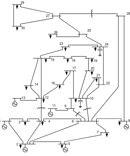
In the study of experiment, MABC algorithm is tested over standard IEEE 30-bus power system with six generating
units as shown in Fig. 1. The parameters of all thermal units are presented in Table 1, followed by B-loss coefficient [9,
The number of colony size, NP = 20; the number of cycles for aging, maxCycle = 300; the number of variables, NV = 6; and limit = 100.
The proposed technique is applied for CEED problem with load demands 500 MW, 700 MW, and 900 MW, respectively and it is compared with FCGA and NSGA-II [25]. Minimum fuel cost solution for CEED problem with all
load demands are considered respectively in Table 2, Table 3, and Table 4. Minimum NOx emission effect solution for
CEED problem with all load demands are considered respectively in Table 5, Table 6, and Table 7. The best compromise solution for CEED problem with all load demands are considered respectively in Table 8, Table 9, and Table 10. 1 2 5 7 8 6 4 3 11 9 10 12 13
14 16 22
21 20 19 18 15 17 23 24 25 26 30 29 27 28
Fig. 1 Single-line diagram of IEEE 30-bus test system [18]
Table 1 Generator capacity limits, fuel cost and emission coefficients for IEEE 30-bus test system
Unit m in
i P (MW) m ax i P (MW) ai
($/MW2)
bi
($/MW)
ci
($)
αi
($/MW2)
βi
($/MW) γi
($)
1 10 125 0.15240 38.53973 756.79886 0.00419 0.32767 13.85932
2 10 150 0.10587 46.15916 451.32513 0.00419 0.32767 13.85932
3 35 225 0.02803 40.39655 1049.9977 0.00683 -0.54551 40.26690
4 35 210 0.03546 38.30553 1243.5311 0.00683 -0.54551 40.26690
5 130 325 0.02111 36.32782 1658.5596 0.00461 -0.51116 42.89553
6 125 315 0.01799 38.27041 1356.6592 0.00461 -0.51116 42.89553
Table 2 Best fuel cost for 6-generator system (PD = 500 MW)
Unit Output FCGA NSGA-II MABC
P1 (MW) 49.47 50.836 52.1024
P2 (MW) 29.40 31.806 29.0471
P3 (MW) 35.31 35.12 40.0000
P4 (MW) 70.42 73.44 68.0901
P5 (MW) 199.03 191.988 191.4150
P6 (MW) 135.22 135.019 136.4637
Fuel cost ($/h) 28150.80 28150.834 28086.9456
Emission (kg/h) 314.53 309.04 306.3324
Power losses (MW) 18.86 18.208 17.1183
Total Capacity (MW) 518.86 518.208 517.1183
Table 3 Best fuel cost for 6-generator system (PD = 700 MW)
Unit Output FCGA NSGA-II MABC
P1 (MW) 72.14 76.179 76.0897
P2 (MW) 50.02 51.81 49.0586
P3 (MW) 46.47 49.82 45.3525
P4 (MW) 99.33 103.407 102.7347
P5 (MW) 264.60 267.984 266.3914
P6 (MW) 203.58 184.734 191.3422
Fuel cost ($/h) 38384.09 38370.746 38207.5910
Emission (kg/h) 543.48 534.924 532.6970
Power losses (MW) 36.15 33.934 30.9692
Total Capacity (MW) 736.14 733.934 730.9692
Table 4 Best fuel cost for 6-generator system (PD = 900 MW)
Unit Output FCGA NSGA-II MABC
P1 (MW) 101.11 102.963 103.4811
P2 (MW) 67.64 74.235 70.1005
P3 (MW) 50.39 66.003 60.6818
P4 (MW) 158.80 140.316 139.5618
P5 (MW) 324.08 324.888 325.0000
P6 (MW) 256.56 248.416 251.7912
Fuel cost ($/h) 49655.40 49620.824 49297.9331
Emission (kg/h) 877.61 849.326 845.6922
Power losses (MW) 58.58 56.822 50.6162
Total Capacity (MW) 958.57 956.822 950.662
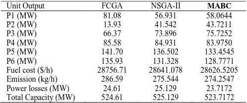
Table 5 Best emission effects for 6-generator system (PD = 500 MW)
Unit Output FCGA NSGA-II MABC
P1 (MW) 81.08 56.931 58.0644
P2 (MW) 13.93 41.542 43.7211
P3 (MW) 66.37 73.896 75.7252
P4 (MW) 85.58 84.931 83.9750
P5 (MW) 141.70 136.502 133.4545
P6 (MW) 135.93 131.328 128.7771
Fuel cost ($/h) 28756.71 28641.078 28626.5205
Emission (kg/h) 286.59 275.544 274.2547
Power losses (MW) 24.61 25.129 23.7172
Table 6 Best emission effects for 6-generator system (PD = 700 MW)
Unit Output FCGA NSGA-II MABC
P1 (MW) 120.16 103.078 105.3292
P2 (MW) 21.36 73.505 76.4086
P3 (MW) 62.09 91.556 92.9206
P4 (MW) 128.05 110.787 109.8345
P5 (MW) 209.65 187.869 183.1928
P6 (MW) 201.12 174.289 170.0132
Fuel cost ($/h) 39455.00 39473.433 39433.4776
Emission (kg/h) 516.55 467.388 462.7169
Power losses (MW) 42.44 41.083 37.6990
Total Capacity (MW) 742.44 741.083 737.6990
Table 7 Best emission effects for 6-generator system (PD = 900 MW)
Unit Output FCGA NSGA-II MABC
P1 (MW) 133.31 124.998 124.9894
P2 (MW) 110.00 109.893 88.3224
P3 (MW) 100.38 111.081 123.9540
P4 (MW) 119.27 141.961 134.8330
P5 (MW) 250.79 254.36 274.6471
P6 (MW) 251.25 226.578 215.4800
Fuel cost ($/h) 53299.64 51254.195 50517.6331
Emission (kg/h) 785.64 760.052 751.2743
Power losses (MW) 65.00 68.87 62.2260
Total Capacity (MW) 965.00 968.87 962.2260
Table 8 Best compromise solution for 6-generator system (PD = 500 MW)
Unit Output FCGA NSGA-II MABC
P1 (MW) 65.23 54.048 54.7203
P2 (MW) 24.29 34.250 32.5975
P3 (MW) 40.44 54.497 49.2279
P4 (MW) 74.22 80.413 77.7303
P5 (MW) 187.75 161.874 166.3428
P6 (MW) 125.48 135.426 137.2141
Fuel cost ($/h) 28231.06 28291.119 28164.7430
Emission (kg/h) 304.90 284.362 282.4029
Power losses (MW) 17.41 20.508 17.1428
Total Capacity (MW) 517.41 520.508 517.1428
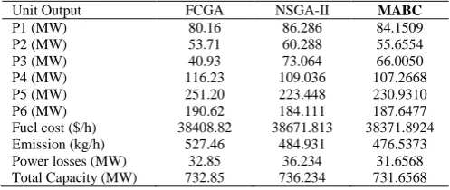
Table 9 Best compromise solution for 6-generator system (PD = 700 MW)
Unit Output FCGA NSGA-II MABC
P1 (MW) 80.16 86.286 84.1509
P2 (MW) 53.71 60.288 55.6554
P3 (MW) 40.93 73.064 66.0050
P4 (MW) 116.23 109.036 107.2668
P5 (MW) 251.20 223.448 230.9310
P6 (MW) 190.62 184.111 187.6477
Fuel cost ($/h) 38408.82 38671.813 38371.8924
Emission (kg/h) 527.46 484.931 476.5373
Power losses (MW) 32.85 36.234 31.6568
Table 10 Best compromise solution for 6-generator system (PD = 900 MW)
Unit Output FCGA NSGA-II MABC
P1 (MW) 111.40 120.052 115.2769
P2 (MW) 69.33 85.203 78.8093
P3 (MW) 59.43 89.565 81.3885
P4 (MW) 143.26 140.278 137.3458
P5 (MW) 319.40 288.614 298.6779
P6 (MW) 252.11 233.687 238.1785
Fuel cost ($/h) 49674.28 50126.059 49553.8355
Emission (kg/h) 850.29 784.696 772.4565
Power losses (MW) 54.92 57.405 49.6769
Total Capacity (MW) 954.92 957.405 949.6769
Summary of the results in Table 2 to Table 10 for the best completion of MABC method compared with NSGA-II in order to reduce fuel costs, emissions, and power losses are shown in Table 11. After comparing the simulation results with the others method, it is obviously seen that proposed MABC algorithm give more powerful results than other algorithms.
Table 11 Summary of MABC VS NSGA-II for 6-generator system
500 700 900
Best fuel cost
Fuel cost ($/h) 63.8884 163.1550 322.8909
Emission (kg/h) 2.7076 2.2270 3.6338
Power losses (MW) 1.0897 2.9648 6.2058
Best emission
Fuel cost ($/h) 14.5575 39.9554 736.5619
Emission (kg/h) 1.2893 4.6711 8.7777
Power losses (MW) 1.4118 3.3840 6.6440
Best compromise
Fuel cost ($/h) 126.3760 299.9206 572.2235
Emission (kg/h) 1.9591 8.3937 12.2395
Power losses (MW) 3.3652 4.5772 7.7281
VI. CONCLUSION
This paper has presented a new optimization algorithm to solve the combined economic emission dispatch problem considering linear equality and inequality constraints and also considering transmission losses. Economic and emission dispatch is a multi-objective problem. But the present approach makes use of only one objective function and depending upon the problem such as economic, emission or combined economic and emission dispatch, only the coefficients of the objective function has to be changed. The feasibility of the proposed method for solving CEED problems is demonstrated using IEEE 30-bus test system with six generating units. The comparison of the results with other methods reported in the literature shows the superiority of the proposed method and its potential for solving CEED problems in a power system. From the results obtained, it can be concluded that the MABC algorithm is a promising technique for solving complex optimization problems in power system operation.
REFERENCES
[1] A.J Wood, B.F. Wollenberg. Power Generation Operation and Control. John Wiley and Sons, New York, 1984. [2] Hadi Saadat. Power System Analysis. Tata McGraw Hill Publishing Company, New Delhi, 2002.
[3] S.Y. Lim, M. Montakhab, H. Nouri, ”Economic Dispatch of Power System using Particle Swarm Optimization with Constriction Factor”, Int. J. Innov. Energy Syst. Power, vol. 4, no. 2, pp. 29-34, 2009.
[4] Z. L. Gaing, ”Particle Swarm Optimization to Solving the Economic Dispatch Considering the Generator Constraints”, IEEE Trans. Power Syst., vol. 18, no. 3, pp. 1187-1195, 2003.
[5] D. C. Walters, G. B. Sheble, ”Genetic Algorithm Solution of Economic Dispatch with Valve Point Loading”, IEEE Trans. Power Syst., vol. 8, no. 3, pp. 1325-1332, 1993.
[6] T. Ratniyomchai, A. Oonsivilai, P. Pao-La-Or, T. Kulworawanichpong, ”Particle Swarm Optimization for Solving Combined Economic and Emission Dispatch Problems”, 5th IASME/WSEAS Int. Conf. Energy Environ, pp. 211-216, 2010.
[7] C. Palanichamy, N. S. Babu, ”Analytical Solution for Combined Economic and Emissions Dispatch”, Elect. Power Systs. Res., vol. 78, pp. 1129-1137, 2008.
[8] N. Cetinkaya, ”Optimization Algorithm for Combined Economic and Emission Dispatch with Security Constraints”, Int. Conf. Comp. Sci. Appl. ICCSA, pp. 150-153, 2009.
[9] R. Balamurugan, S. Subramanian, ”A Simplified Recursive Approach to Combined Economic Emission Dispatch”, Elec. Power Comp. Syst., vol. 36, no. 1,pp. 17-27, 2008.
[10] L. Abdelhakem Koridak, M. Rahli, M. Younes, ”Hybrid Optimization of the Emission and Economic Dispatch by the Genetic Algorithm”, Leonardo Journal of Sciences, Issue 14, pp. 193-203, 2008.
[11] U. Güvenç, ”Combined Economic Emission Dispatch Solution using Genetic Algorithm Based on Similarity Crossover”, Sci. Res. Essay, vol. 5, no. 17, pp. 2451-2456, 2010.
[12] Simon Dinu, Ioan Odagescu, Maria Moise, ”Environmental Economic Dispatch Optimization using a Modified Genetic Algorithm”, International Journal of Computer Applications, vol. 20, no. 2, pp. 7-14, 2011.
[13] J. Sasikala, M. Ramaswamy, ”Optimal λ Based Economic Emission Dispatch using Simulated Annealing”, Int. J. Comp. Appl., vol. 1, no. 10, pp. 55-63, 2010.
[14] P. K. Roy, S. P. Ghoshal, S. S. Thakur, ”Combined Economic and Emission Dispatch Problems using Biogeography-Based Optimization”, Electr. Eng., vol. 92, no. 4-5, pp. 173-184, 2010.
[15] Y. M. Chen, W. S. Wang, ”Particle Swarm Approach to Solve Environmental/Economic Dispatch Problem”, International Journal of Industrial Engineering Computations, vol. 1, pp. 157-172, 2010.
[16] Anurag Gupta, K. K. Swarnkar, K. Wadhwani, ”Combined Economic Emission Dispatch Problem using Particle Swarm Optimization”, International Journal of Computer Applications, vol. 49, no. 6, pp. 1-6, 2012.
[17] S. Hemamalini, S. P. Simon, ”Economic/Emission Load Dispatch using Artificial Bee Colony Algorithm’, Int. Conf. Cont., Comm. Power Eng., pp. 338-343, 2010.
[18] Y. Sonmez, ”Multi-Objective Environmental/Economic Dispatch Solution with Penalty Factor using Artificial Bee Colony Algorithm”, Sci. Res. Essay, vol. 6, no. 13, pp. 2824-2831, 2011.
[19] D. Karaboga, B. Basturk, ”On the Performance of Artificial Bee Colony (ABC) Algorithm”, Applied Soft Computing, vol. 8, no. 1, pp. 687- 697, 2008.
[20] D. Karaboga, B. Akay, ”Artificial Bee Colony (ABC), Harmony Search and Bees Algorithms on Numerical Optimization”, Proceedings of IPROMS 2009 Conference, pp. 1-6, 2009.
[21] B. Akay, D. Karaboga, ”A Modified Artificial Bee Colony Algorithm for Real-Parameter Optimization”, Information Sciences, vol. 192, pp. 120-142, 2012.
[22] X. T. Li, X. W. Zhao, J. N. Wang, M. H. Yin, ”Improved Artificial Bee Colony for Design of a Reconfigurable Antenna Array with Discrete Phase Shifters”, Progress in Electromagnetics Research C, vol. 25, pp. 193-208, 2012.
[23] R. Storn, K. Price, “Differential Evolution a Simple and Efficient Heuristic for Global Optimization Over Continuous Spaces”, Journal of Global Optimization, vol. 11, no. 4, pp. 341-359, 1997.
[24] K. Price, R. Storn, J. A. Lampinen. Differential Evolution: A Practical Approach to Global Optimization. Springer, Berlin, Heidelberg, 2005. [25] HCS Rughooputh, RTFA King, “Environmental/Economic Dispatch of Thermal Units using an Elitist Multi-Objective Evolutionary Algorithm”,
IEEE Int. Conf. Ind. Tech., pp. 48-53, 2003.
BIOGRAPHY
Hardiansyah was born on February 27, 1967 in Mempawah, Indonesia. He received the B.S. degree in Electrical Engineering from the University of Tanjungpura in 1992 and the M.S. degree in Electrical Engineering from Bandung Institute of Technology (ITB), Indonesia in 1996. Dr. Eng, degree from Nagaoka University of Technology in 2004. Since 1992, he has been with Department of Electrical Engineering, University of Tanjungpura, Pontianak, Indonesia. Currently, he is a senior lecturer in Electrical Engineering. His current research interests include power system operation and control, robust control, and soft computing techniques in power system.