COMPARISON OF THE RADIATION PATTERN OF FRACTAL AND CONVENTIONAL LINEAR ARRAY ANTENNA
R. T. Hussein and F. J. Jibrael
Electrical and Electronic Engineering Department University of Technology
Baghdad, Iraq
Abstract—The purpose of this paper is to introduce the concept of fractals and its use in antenna arrays for obtaining multiband property. One type of fractals namely, Cantor set is investigated. Cantor set is used in linear array antenna design. Therefore, this array know fractal Cantor linear array antenna. A comparison with conventional non-fractal linear array antenna is made regarding the beamwidth, directivity, and side lobe level. MATLAB programming language version 7.2 (R2006a) is used to simulate the fractal and conventional non-fractal linear array antenna and their radiation pattern.
1. INTRODUCTION
new solution to the design of multiband antennas and arrays. Fractal geometries have found an intricate place in science as a representation of some of the unique geometrical features occurring in nature. Fractal was first defined by Benoit Mandelbrot [2] in 1975 as a way of classifying structures whose dimensions were not whole numbers. These geometries have been used previously to characterized unique occurrences in nature that were difficult to define with Euclidean geometries, including the length of coastlines, the density of clouds, and branching of trees [3]. Fractals can be divided into many types, as shown in Fig. 1.
(a) (b) (c)
(d)
Figure 1. Three fractal examples. (a) Sierpinski gasket. (b) Koch snowflake. (c) Tree. (d) Cantor set.
2. CONVENTIONAL LINEAR ARRAY ANTENNA
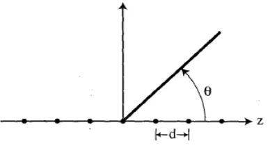
An array is usually comprised of identical elements position in a regular geometrical arrangement. A linear array of isotropic elements N, uniformly spaced a distance d apart along the z-axis, is shown in Fig. 2 [4].
The array factor corresponding to this linear array may be expressed in the form [1, 5]
AF(ψ) =
a0+ 2
N
n=1
ancos (nψ) for (2N+ 1) elements
2 N
n=1
ancos
2n−1
2
ψ for (2N) elements
(1)
ψ = kdcosθ+α (2)
k = 2π
λ (3)
AF(ψ) = the array factor
d= spacing between adjacent elements in the array
α = the progressive phase shift between elements
k= 2λπ = the wave number
θ= elevation angle
3. FRACTAL LINEAR ARRAY ANTENNA
Fast recursive algorithms for calculating the radiation patterns of fractal arrays have recently been developed in [6–8]. These algorithms are based on the fact that fractal arrays can be formed recursively through the repetitive application of a generating array. A generating array is a small array at level one (P = 1) used to recursively construct larger arrays at higher levels (i.e., P > 1). In many cases, the generating subarray has elements that are turned on and off in a certain pattern. A set formula for copying, scaling, and translating of the generating array is then followed in order to produce a family of higher order arrays.
The array factor for a fractal antenna array may be expressed in the general form [6–8]
AFP =
P
p=1
GAδp−1ψ (4)
where GA(ψ) represents the array factor associated with the generating array. The parameterδ is a scaling or expansion factor that governs how large the array grows with each successive application of the generating array and P is a level of iteration.
This arrays become fractal-like when appropriate elements are turned off or removed, such that
an=
1 if elementnis turned on 0 if elementnis turned off
One of the simplest schemes for constructing a fractal linear array follows the recipe for the cantor set [9]. Cantor arrays own also multiband properties, so it has multi frequencies (Fn):
Fn=
F0
δn n= 0,1,2, . . . , P−1 (5)
whereF0 is the design frequency.
iteration 0
iteration 2 iteration 1
iteration 4 iteration 3
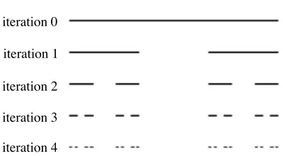
Figure 3. The first four iterations in the construction of the Cantor set array.
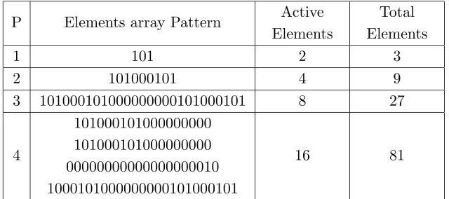
The basic Cantor array, as shown in Fig. 3 may be created by starting with a three element generating subarray, and then applying it repeatedly over P scales of growth. The generating subarray in this case has three uniformly spaced elements, with the center element turned off or removed, i.e., 101. The Cantor array is generated recursively by replacing 1 by 101 and 0 by 000 at each level of the construction. Table 1 provides the array pattern for the first four levels of the Cantor array.
The array factor of the three element generating subarray with the representation 101 is
GA(ψ) = 2 cos (ψ) (6)
which may be derived from Eq. (1) by setting N = 1, a0 = 0.
Substituting Eq. (6) into Eq. (4) and choosing an expansion factor of three (δ = 3), the results in an expression for the Cantor array factor given by
AFP(ψ) =
P
p=1 GA
3p−1ψ
= 2 P p=1 cos
3p−1ψ
Table 1. First four levels of the fractal Cantor linear array.
P Elements array Pattern Active Elements
Total Elements
1 101 2 3
2 101000101 4 9
3 101000101000000000101000101 8 27
4
101000101000000000 101000101000000000 00000000000000000010 1000101000000000101000101
16 81
4. COMPUTER SIMULATION RESULTS
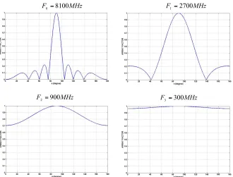
In this work, MATLAB programming language version 7.2 (R2006a) used to simulate and design the conventional and fractal linear array antenna and their radiation pattern. Let, a linear array will be design and simulate at a frequency F0 equal to 8100 MHz, (then
the wavelength λ0 = 0.037 m), with quarter-wavelength (d = λ0/4)
Table 2. SLL,D, and HP BW for fractal linear array antenna.
F (MHz) D (dB) HP BW (degree) SLLmax (dB)
8100 12.0436 2.0233 −5.451
2700 9.1969 6.0721 −5.446
900 6.204 18.2852 −5.446
300 3.1848 56.9372 −∞
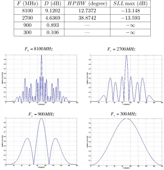
Table 3. SLL,D, andHP BW for conventional linear array antenna.
F (MHz) D (dB) HP BW (degree) SLLmax (dB)
8100 9.1202 12.7372 −13.148
2700 4.6369 38.8742 −13.593
900 0.893 — −∞
300 0.106 — −∞
MHz
F2=900 F3=300MHz
MHz
F0 =8100 F1=2700MHz
F0 =8100MHz F1=2700MHz
MHz
F2=900 F3=300MHz
Figure 5. Array factor of a conventional non-fractal linear array antenna.
5. CONCLUSION
At design frequencyF0= 8100 MHz, the field pattern for conventional
REFERENCES
1. Balanis, C. A., Antenna Theory: Analysis and Design, 2nd edition, Wiley, 1997.
2. Mandelbrot, B. B., The Fractal Geometry of Nature, W. H. Free-man and Company, New York, 1983.
3. Gianvittorio, J., “Fractal antennas: Design, characterization and application,” Master’s Thesis, University of California, Los Angeles, 2000.
4. Werner, D. H., R. L. Haupt, and P. L. Werner, “Fractal antenna engineering: The theory and design of fractal antenna arrays,”
IEEE Antennas and Propagation Magazine, Vol. 41, No. 5, 37–59,
October 1999.
5. Stutzman, W. L. and G. A. Thiele, Antenna Theory and Design, 2nd edition, John Wiley & Sons, New York, 1998.
6. Baliarda, C. P. and R. Pous, “Fractal design of multi-band and low side-lobe arrays,” IEEE Transactions on Antennas and
Propagation, Vol. 44, No. 5, 730–739, May 1996.
7. Werner, D. H. and R. L. Haupt, “Fractal construction of linear and planar arrays,”Proceedings IEEE Antennas Propagation Soc.
Int. Symp., Vol. 3, 1968–1971, July 1997.
8. Werner, D. H. and R. Mittra,Frontiers in Electromagnetics, IEEE Press, 2000.
9. Peitgen, H. O., H. Jurgens, and D. Saupe, Chaos and Fractals: