R E S E A R C H
Open Access
Identification of MIMO systems with sparse
transfer function coefficients
Wanzhi Qiu
*, Syed Khusro Saleem and Efstratios Skafidas
Abstract
We study the problem of estimating transfer functions of multivariable (multiple-input multiple-output–MIMO) systems with sparse coefficients. We note that subspace identification methods are powerful and convenient tools in dealing with MIMO systems since they neither require nonlinear optimization nor impose any canonical form on the systems. However, subspace-based methods are inefficient for systems with sparse transfer function coefficients since they work on state space models. We propose a two-step algorithm where the first step identifies the system order using the subspace principle in a state space format, while the second step estimates coefficients of the transfer functions via L1-norm convex optimization. The proposed algorithm retains good features of subspace methods with improved noise-robustness for sparse systems.
Keywords:system identification, MIMO system, sparse representation, L1-norm optimization
1. Introduction
The problem of identifying multiple-input multiple-out-put (MIMO) systems arises naturally in spatial division multiple access architectures for wireless communica-tions. Subspace system identification methods refer to the category of methods which obtain state space mod-els from subspaces of certain matrices constructed from the input-output data [1]. Being based on reliable numerical algorithms such as the singular value decom-position (SVD), subspace methods do not require non-linear optimization and, thereby, are computationally efficient and stable without suffering from convergence problems. They are particularly suitable for identifying MIMO systems since there is no need to impose on the system a canonical form and, therefore, they are free from the various inconveniences encountered in classical parametric methods.
Another good feature of subspace methods is they incorporate a reliable order estimation process. Although this is largely ignored by other identification methods, system order estimation should be an integral part of a system identification algorithm. In fact, cor-rectly identifying the system order is essential to ensure that subsequent parameter estimation will yield a
well-defined set of model coefficient estimates. While it is obvious that an underestimated order will result in large modeling errors, it is equally dangerous to have an over-parameterized model as a result of selecting an impro-perly large order. Over-parameterization not only cre-ates a larger set of parameters to be estimated, but also leads to poorly defined (high variance) coefficient esti-mates and surplus unvalidated content in the resulting model [2]. For parameterized linear models, a usual way of estimating the order is to conduct a series of tests on different orders, and select the best one based on the goodness-of-fit using certain criterion such as the Akaike’s information criterion [3]. Subspace-based order identification determines the order as the number of principle eigenvalues (or singular values) of a certain input-output data matrix. This mechanism has been proven to be a simple and reliable way of order estima-tion and the same principle has been applied to detect the number of emitter sources in array signal processing [4], to determine the number of principal components in signal and image analysis [5,6] and to estimate the system order in blind system identification [7,8].
It has become well known that many systems in real applications actually have sparse representations, i.e., with a large portion of their transfer function coeffi-cients equal to zero [9]. For example, communication channels exhibit great sparseness. In particular, in high-* Correspondence: [email protected]
National ICT Australia, Department of Electrical and Electronic Engineering, The University of Melbourne, Parkville, VIC 3010, Australia
definition television, there are few echoes but the chan-nel response spans many hundreds of data symbols [10-12]. In broadband wireless communications, a hilly terrain delay profile consists of a sparsely distributed multipath [13]. Underwater acoustic channels also exhi-bit sparseness [14].
Despite of their good features, subspace methods are not suited for systems with sparse transfer function coefficients since they deal with state space models. One fact is that for a given transfer function matrix, there exist infinite number of state space representations related by a similarity transform. As a result, when the system to be identified has sparse transfer function coef-ficients, the state space model produced by a subspace method is almost certain to be non-sparse due to the inherent arbitrary similarity transform associated with the model.
Work on sparse system identification has been reported in [15-17], however, they consider only single-input single-out (SISO) systems. In addition, these methods assume the system order is known a priori, which is not necessarily true in practice. This article stu-dies the problem of the identification of MIMO systems with sparse transfer functions coefficients. In particular, we leverage on reliable system order identification of subspace methods to build input-output relationship in terms of transfer function coefficients, and exploit L1-norm optimization proven to be able to produce robust sparse solutions [9] to estimate these coefficients. The resulting method consists of a systematic way of order identification and efficient coefficient estimation for sparse systems.
The rest of this article is organized as follows. Section 2 gives an overview of subspace identification methods. Section 3 proposes the LRL1 algorithm. Section 4 pre-sents simulation results and Section 5 draws conclusions.
2. Subspace identification
For an M-input {um(k),m= 1,...,M}L-output {yl(k),l= 1,...,L} system described in the state space form:
xk+1=Axk+Buk (1a)
yk=Cxk+Duk (1b)
where ukdef= [u1(k),. . .,uM(k)]T,
ykdef= [y1(k),. . .,yL(k)]T, and xk
def
= [x1(k),. . .,xN(k)]T are the input, output, and state vectors, respectively, with T denoting matrix transpose. A Î RN×N, B Î
RN×M, C Î RL×N, andD Î RL×Mare the system, input,
output, and direct feed-through matrices, respectively.
Noise in (1) has been omitted for brevity purposes and will be added in the simulation in Section 4. Given S measurements (i.e.,k= 0,...,S - 1) of the input and out-put, subspace identification methods estimate the system order Nand matrices (A, B, C, D), and derive system transfer functions via H(z) =D +C(zINN- A)-1B, with
INNdenoting the identity matrix of sizeN×N. The
pro-cedure is as follows.
Choose a positive integer iand define the input and output block Hankel matrices as:
U0/i−1=
⎛ ⎜ ⎜ ⎜ ⎝
u0u1 · · · uj−1 u1u2 · · · uj
· · · ·
ui−1ui · · · ui+j−2
⎞ ⎟ ⎟ ⎟
⎠ (2)
Y0/i−1=
⎛ ⎜ ⎜ ⎜ ⎜ ⎝
y0y1 · · · yj−1
y1y2 · · · yj
· · · ·
yi−1yi · · · yi+j−2
⎞ ⎟ ⎟ ⎟ ⎟ ⎠
Note that U0/i-1hasj (=S- i + 2) columns with the
first one formed byuk(k= 0,...,i - 1). Similarly, we can
define thej-column block Hankel matrix Ui/2i-1 usinguk
(k=i,..., 2i- 1) to form the first column. For conveni-ence, the following short-hand notations are adopted:
Up
def
= U0/i−1, Yp
def
=Y0/i−1 (3)
Uf
def
= Ui/2i−1, Yf
def
= Yi/2i−1 (4)
For each of the four matrices in (3) and (4), by delet-ing or adddelet-ing one block row at the bottom and keepdelet-ing the number of columns unchanged, we have two addi-tional notations. For example,
Y−f def=Yi/2i−2, Y+f
def
= Yi/2i
Note that i is a user-specified parameter and is required to be larger than the system order, i.e.,i>N. In general, a subspace identification algorithm consists of three steps. The first step performs projections of the row spaces of the data matrices and estimates the order of the system. In particular, the following oblique pro-jections are first calculated:
Oi=Yf/UfWp (5)
where Wp=
Up
Yp , W
+
p=
U+p
Y+p
, and Yf/UfWp are the oblique projection of the row space ofYfalong the row space ofUfon the row space ofWpand can be cal-culated according to
Yf/UfWp= [Yf/U T
f]·[Wp/UTf]·Wp
with [Yf/UTf] denoting the projection of the row space ofYfon the row space of the orthogonal compliment of
the row space ofUf[1].
The SVD of the weighted oblique projection is calcu-lated and the order of the system (N) is determined as the number of principal singular vales in Σ, leading to the identification of the principal subspacesU1 andV1,
W1OiW2=UV= (U1U2)
1 0
0 2
VT
1
VT2
=U11VT1(6)
whereW1and W2are weighting matrices and a
speci-fic choice of them leads to different algorithms [1]. For example,
W1=IiL, W2=Ij (7)
and
W1=IiL, W2= (U⊥f )T(U⊥f (U⊥f )T)†U⊥f , (8) result in the popular N4SID and MOESP algorithms, respectively, with † denoting Moore-Penrose pseudo-inverse.
Define the extended observability matrix and state sequence as
i
def
=
⎛ ⎜ ⎜ ⎜ ⎜ ⎜ ⎝
C CA
.. .
CAi−1
⎞ ⎟ ⎟ ⎟ ⎟ ⎟ ⎠
Xi
def
= (xixi+1,. . .,xi+j−1)∈RN×j.
The second step of a subspace algorithm is to find estimates of the extended observability matrix and state sequences via
i=W−11U11/21
Xi=i†Oi, Xi+1=i†−1Oi+1
The final step is to determine the system matrices A,
B, C, and D(up to within a similarity transformation) by
min
A,B,C,D
Xi+1 Yi/i
−
A B C D
Xi
Ui/i
2
F
. (9)
Note that the sizes of matrices involved in the sub-space methods are dependant on i. It will be shown in Section 4 that while the order can be estimated reliably across a broad range ofi’s as long as the conditioni>N is satisfied, the quality of subsequent coefficient esti-mates depends oniin a non-monotonous fashion.
3. The proposed LRL1
As mentioned previously, subspace methods are ineffi-cient in dealing with sparse transfer function coeffi-cients. That is, for a system with sparse transfer function coefficients, the outcome of subspace methods is one of many (non-sparse) state space realizations (A,
B, C, D). In order to exploit the sparseness in the sys-tem, system (1) is represented using transfer function coefficients. In particular, for thelth output the follow-ing linear regression (LR) relationship holds:
yl(k+N) = N
n=1
anyl(k+N−n)
+
M
m=1
N
n=0
bmn,lum(k+N−n), k= 1,. . .,S−N,l= 1,. . .,L, (10)
Where{an, bmn, l} are the system transfer function coefficients. Equation (10) can be re-written into a vec-tor form:
yl(k+N) =yTk,la+ M
m=1
bTm,lumk, k= 1,. . .,S−N,(11)
where
a= (a1. . .aN)T, (12)
yTk,l=yl(k+N−1),yl(k+N−2),. . .,yl(k)
,
uTmk=um(k+N),um(k+N−1),. . .,um(k)
,
and the contribution of the mth input to thelth out-put is presented by
yl= [YlU]γl, (14) where
yl= [yl(N+ 1)yl(N+ 2). . .yl(S)]T,
U=(U1. . .UM),
Yl= ⎛ ⎜ ⎜ ⎜ ⎜ ⎜ ⎝
yT1,l
yT2,l
.. .
yTS−N,l
⎞ ⎟ ⎟ ⎟ ⎟ ⎟ ⎠
, Um= ⎛ ⎜ ⎜ ⎜ ⎜ ⎜ ⎝
uTm1
uTm2
.. .
uTm(S−N)
⎞ ⎟ ⎟ ⎟ ⎟ ⎟ ⎠
,
γl= (aT βTl)T,
βl= (bT1,l. . .b T M,l)T,
Note that it is a common practice to identify a multi-input single-output model for each output separately and then combine the individual models into a final MIMO model. However, if there are common or corre-lated parameters among models for different output variables and/or correlated noise, then performing iden-tification on all outputs simultaneously can lead to bet-ter and more robust models [18]. By combining all outputs of (14), we have
y=Hβ (15)
where
y=
⎛ ⎜ ⎜ ⎜ ⎜ ⎜ ⎝
y1 y2
.. .
yL
⎞ ⎟ ⎟ ⎟ ⎟ ⎟ ⎠
, β=
⎛ ⎜ ⎜ ⎜ ⎜ ⎜ ⎜ ⎜ ⎝
a
β1
β2
.. .
βL ⎞ ⎟ ⎟ ⎟ ⎟ ⎟ ⎟ ⎟ ⎠
,
H=
⎛ ⎜ ⎜ ⎜ ⎝
Y1U 0· · · 0 Y2 0 U 0· · · 0
· · · ·
YL 0 · · · 0 U ⎞ ⎟ ⎟ ⎟ ⎠.
We now propose a two-step algorithm which first identifies the system order in state space format. This allows the formation of a MIMO model in terms of transfer function coefficients. L1-norm optimization is then exploited to estimate the coefficients of the model. One of the key factors leading to recent advances in
compressed sensing (CS) is that L1-norm optimization promotes sparsity. That is, as compared with its popular L2-norm counterpart, L1-norm optimization produces better results when the parameters to be estimated are sparse [9]. In our case, the data model (15) allowsbto be obtained by L1-norm minimization with guaranteed convergence since, unlike the cases in CS, this is strict convex optimization. The minimization generally takes the following form [19]:
∧
β= arg min
x (||x||1+λ||y−Hx|| 2
2) (16)
Where lbalances the sparsity of the solution with the fidelity to the data and should be inversely proportional to the noise level. Efficient algorithms for solving (16) have been developed [9,19].
The proposed algorithm makes further use of the SVD in (6), where matrixΣ1= diag(l1,...,lN)contains the
prin-cipal singular-values andΣ2= diag(lN+1,...,liL)contains
noise singular-values. When noise is absent,Σ2is an
all-zero matrix. Otherwise, its diagonal entries will be non-zero positive numbers. Although it is impossible here to accurately estimate the noise variance, these diagonal entries do reflect the noise level and can be represented by
¯
σ=
iL
k=N+1
λ2
k
/(iL−N) (17)
In our proposed method, we will set the parameter in (16) to λ=δ/σ¯ where δis a positive constant. The pro-posed LRL1 algorithm can now be summarized as follows:
Step 1: Subspace identification of system order using (5) and (6), and estimation of noise level using (17). This step is a systematic order selection procedure with reliable performance.
Step 2: Estimation of system transfer function coeffi-cients using (16). This step is simultaneous optimization over all outputs with robust sparse solutions.
4. Simulation
We evaluate the performances of the proposed LRL1 method against that of the subspace method N4SID [1]. The first MIMO system under consideration is gener-ated by modifying the SISO system in [[1], p. 155]. In particular, the system order and eigenvalues (i.e., the vector [1aT]T)are kept unchanged and one more input and one more output are added to the original system. Then, some elements in each of the transfer function vectorbm,l(see (13)) are set to zero to create the desired sparsity. The resulting 2-input 2-output system of order
System 1:
a= (0 0 0 0.5288)T,
⎛ ⎜ ⎜ ⎜ ⎜ ⎝
bT1,1
bT2,1
bT1,2
bT2,2
⎞ ⎟ ⎟ ⎟ ⎟ ⎠=
⎛ ⎜ ⎜ ⎜ ⎝
- 0.7139 0 1.2080 0 - 4.0361 0 2.9505 - 2.7061 0 0.5238 0 0.0526 - 0.0239 - 0.6024 0 0 - 0.2686 - 0.2374 0.1585 0
⎞ ⎟ ⎟ ⎟ ⎠.
In the simulation, the data size is chosen to be S = 200 and the inputs are sequences of Gaussian variables with zero mean and unit variance. A white noise vector
vk is added to the output vector yk (see (1b)) and the
SNR as defined below is kept constant for eachk,
SNR = ||yk||
2
||vk||2
.
100 runs are conducted for each simulated scenario, where for each run the input and noise vectors are inde-pendently generated. The root mean square error (RMSE) for the estimates of the T =N +M(N+ 1)L parameters inbis measured as
RMSE =
1
100T 100
r=1
||β(r)−β||22
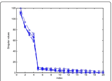
whereb(r) denotes the estimates in therth run. In the simulation,δ= 0.5 is fixed for all the scenarios and the con-vex programming package from [20] is used in solving (16). As mentioned in Section 2, the subspace approach identifies the system order (N) by examining theiL diag-onal entries of Σ in (6), i.e., the singular values (l1,...,
liL) of the system, where iis the number of block rows
of the Hankel data matrices (see (2)) and L= 2 is the number of outputs. For SNR = 30 and ichanging from 4 to 10, we obtainiLsingular values for each particular choice ofi. Figure 1 shows (l1,..., liL, 0,..., 0) where zero padding is made for cases withi< 10.
Checking for the number of principal (dominant) singu-lar values clearly indicates that the system order isN= 4. This result verifies that the identification of system order is reliable regardless of the value ofias long as it is chosen to be larger thanN. This feature is very attractive in practice since it is relatively easy to select aniwhich is larger than the largest possible value the system order might have.
Having identified the system order, we now follow the subsequent steps of the subspace and proposed LRL1 methods to estimate model coefficients. Figure 2 shows the RMSE of the subspace method wheni changes from 5 to 10 at SNR = 30. It can be seen here that the perfor-mance of the subspace method depends oniin a
non-monotonous fashion. That is, a larger idoes not neces-sarily leads to better coefficient estimates. This is due to the fact that only finite datasets are available; increasing the number of rows of the data matrices will lead to a reduction in the number of columns. In the subsequent simulations,i= 9 is used.
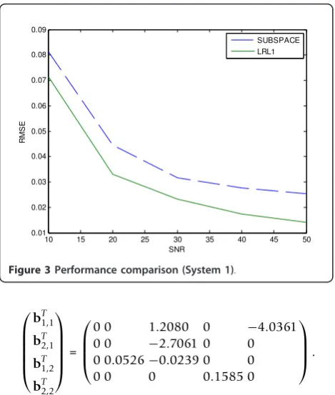
Figure 3 compares the estimation errors of the sub-space and LRL1 methods for different SNR values. The results show that LRL1 is more robust to noise in deal-ing with this sparse system.
Further test is conducted by modifying System 1 to create an even sparser system. In particular, some of the transfer function coefficients ofSystem 1are set to zero, which results in
System 2:
a= (0 0 0 0.5288)T,
0 2 4 6 8 10 12 14 16 18 20 0
20 40 60 80 100 120
index
S
ingul
ar
v
al
ues
Figure 1System singular values (System 1).
5 5.5 6 6.5 7 7.5 8 8.5 9 9.5 10 0.0322
0.0324 0.0326 0.0328 0.033 0.0332 0.0334 0.0336 0.0338 0.034 0.0342
i
RM
S
E
SUBSPACE
⎛ ⎜ ⎜ ⎜ ⎜ ⎝
bT1,1
bT2,1
bT1,2
bT2,2
⎞ ⎟ ⎟ ⎟ ⎟ ⎠=
⎛ ⎜ ⎜ ⎝
0 0 1.2080 0 −4.0361 0 0 −2.7061 0 0 0 0.0526−0.0239 0 0 0 0 0 0.1585 0
⎞ ⎟ ⎟ ⎠.
Figure 4 shows the performances of the two methods under the same conditions as in Figure 3. The results demonstrate that the improvement of LRL1 over the original subspace method increases when the system to be identified becomes sparser.
5. Conclusion
A noise-robust algorithm for the identification of MIMO systems has been presented. The proposed method leverages reliable system order identification of subspace principle and exploits L1-norm optimization to achieve high effectiveness for identifying systems with
sparse transfer function coefficients. While retaining good features of original subspace methods such as the convenience for multivariable systems, the proposed method is shown to be able to significantly improve estimation accuracy for sparse systems.
Competing interests
The authors declare that they have no competing interests.
Received: 9 January 2012 Accepted: 9 May 2012 Published: 9 May 2012
References
1. P Vanoverschee, B DeMoor,Subspace Identification for Linear Systems: Theory-Implementation-Applications(Springer, 1996).
2. P Young,Recursive Estimation and Time-series Analysis: An Introduction
(Springer, 1984)
3. H Akaike, A new look at the statistical model identification. IEEE Trans Autom Control.19(6), 716–723 (1974)
4. S Ouyang, Y Hua, Bi-iterative least square method for subspace tracking. IEEE Trans Signal Process.53(8), 2984–2996 (2005)
5. W Qiu, E Skafidas, Robust estimation of GCD with sparse coefficients. Signal Process.90(3), 972–976 (2010)
6. H Andrews, C Patterson, Singular value decompositions and digital image processing. IEEE Trans Acoust Speech Signal Process.24(1), 26–53 (2003) 7. KA Meraim, W Qiu, Y Hua, Blind system identification. Proc IEEE.85(8),
1310–1322 (1997)
8. W Qiu, SK Saleem, M Pham, Blind identification of multichannel systems driven by impulsive signals. Digital Signal Process.20(3), 736–742 (2010) 9. E Candès, M Wakin, An introduction to compressive sampling. IEEE Signal
Process Mag.25(2), 21–30 (2008)
10. SF Cotter, BD Rao, Sparse channel estimation via matching pursuit with application to equalization. IEEE Trans Commun.50(3), 374–377 (2002) 11. WF Schreiber, Advanced television systems for terrestrial broadcasting: some problems and some proposed solutions. Proc IEEE.83, 958–981 (1995)
12. IJ Fevrier, SB Gelfand, MP Fitz, Reduced complexity decision feedback equalization for multipath channels with large delay spreads. IEEE Trans Commun.47, 927–937 (1999)
13. S Ariyavisitakul, NR Sollenberger, LJ Greenstein, Tap selectable decision-feedback equalization. IEEE Trans Commun.45, 1497–1500 (1997) 14. M Kocic, D Brady, M Stojanovic, Sparse equalization for real-time digital
underwater acoustic communications, inProc OCEANS95, San Diego, CA, pp. 1417–1422 (October 1995)
15. Y Chen, Y Gu, AO Hero III, Sparse LMS for system identification, in
Proceedings of ICASSP, Taipei, Taiwan, pp. 3125–3128 (19-24 April 2009) 16. M Sharp, A Scaglione, Application of sparse signal recovery to pilot-assisted
channel estimation, inProc of Intl Conf on Acoustics, Speech and Signal Proc, Las Vegas, NV, (April 2008)
17. M Sharp, A Scaglione, Estimation of sparse multipath channels, in
Proceedings of IEEE Military Communications Conference, San Diego, CA, pp. 1–7 (17-19 November 2008)
18. BS Dayal, JF MacGregor, Multi-output process identification. J Process Control Elsevier Sci.7(4), 269–282 (1997)
19. E Candès, T Tao, The Dantzig selector: statistical estimation whenpis much larger than n. Ann Stat.35, 2313–2351 (2005)
20. M Grant, S Boyd, CVX: Matlab software for disciplined convex programming (web page and software). http://stanford.edu/~boyd/cvx. Accessed 12 January 2012
doi:10.1186/1687-6180-2012-104
Cite this article as:Qiuet al.:Identification of MIMO systems with sparse transfer function coefficients.EURASIP Journal on Advances in Signal Processing20122012:104.
10 15 20 25 30 35 40 45 50
0.005 0.01 0.015 0.02 0.025 0.03 0.035 0.04 0.045 0.05
SNR
RM
S
E
SUBSPACE LRL1
Figure 4Performance comparison (System 2).
10 15 20 25 30 35 40 45 50
0.01 0.02 0.03 0.04 0.05 0.06 0.07 0.08 0.09
SNR
RM
S
E
SUBSPACE LRL1