Blind source separation for robot audition using fixed HRTF beamforming

(1)

R E S E A R C H

Open Access

Blind source separation for robot audition using

fixed HRTF beamforming

Mounira Maazaoui

*

, Karim Abed-Meraim and Yves Grenier

Abstract

In this article, we present a two-stage blind source separation (BSS) algorithm for robot audition. The first stage consists in a fixed beamforming preprocessing to reduce the reverberation and the environmental noise. Since we are in a robot audition context, the manifold of the sensor array in this case is hard to model due to the presence of the head of the robot, so we use pre-measured head related transfer functions (HRTFs) to estimate the

beamforming filters. The use of the HRTF to estimate the beamformers allows to capture the effect of the head on the manifold of the microphone array. The second stage is a BSS algorithm based on a sparsity criterion which is the minimization of thel1norm of the sources. We present different configuration of our algorithm and we show that it has promising results and that the fixed beamforming preprocessing improves the separation results.

1 Introduction

Robot audition consists in the aptitude of an humanoid to understand its acoustic environment, separate and localize sources, identify speakers and recognize their emotions. This complex task is one of the target points

of the Romeo projecta that we work on. This project

aims to build an humanoid (Romeo) that can act as a comprehensive assistant for persons suffering from loss of autonomy. Our task in this project is focused on the blind source separation (BSS) topic using a microphone array (more than two sensors). Source separation is a very important step for human-robot interaction: it allows latter tasks like speakers identification, speech and motion recognition and environmental sound analy-sis to be achieved properly. In a BSS task, the separation should be done from the received microphone signals without prior knowledge of the mixing process. The only knowledge is limited to the array geometry.

The problem of BSS has been studied by many authors [1], and we present here some of the state-of-the-art methods related to robot audition. Tamai et al. [2] performed sound source localization by a delay and sum beamforming and source separation in a real envir-onment with frequency band selection using a

micro-phone array located on three rings with 32

microphones. Yamamoto et al. [3] proposed a source

separation technique based on geometric constraints as a preprocessing for the speech recognition module in their robot audition system. This system was implemen-ted in the humanoids SIG2 and Honda ASIMO with an eight sensors microphone array, as a part of a more complete system for robot audition named HARK [4]. Saruwatari et al. [5] proposed a two-stage binaural BSS system for an humanoid. They combined a single-input multiple-output model based on independent compo-nent analysis (ICA) and a binary mask processing.

One of the main challenges of BSS remains to obtain good BSS performance in a real reverberant environ-ments. A beamforming preprocessing can be a solution to improve BSS performance in a reverberant room. Beamforming consists in estimating a spatial filter that operates on the outputs of a microphone array in order to form a beam with a desired directivity pattern [6]. It is useful for many purposes, particularly for enhancing a desired signal from its measurement corrupted by noise, competing sources and reverberation [6]. Beamforming filters can be estimated in a fixed or in an adaptive way. A fixed beamforming, contrarily to an adaptive one, does not depend on the sensors data, the beamformer is built for a set of fixed desired directions. In this article, we propose a two-stage BSS technique where a fixed beamforming is used in a preprocessing step.

Ding et al. propose to use a beamforming preproces-sing where the steering directions are the directions of arrival (DOA) of the sources. In this case, the DOA of

* Correspondence: [email protected]

Institute Telecom, Telecom ParisTech, CNRS-LTCI 37/39, rue Dareau, 75014, Paris, France

(2)

the sources are supposed to be knowna priori [7]. The authors evaluate their method in a determined case with 2 and 4 sources and a circular microphone array. Saru-watari et al. present a combined ICA [8] and beamform-ing method: first the authors perform a subband ICA and estimate the direction of arrivals (DOA) of the sources using the directivity patterns in each frequency bin, second they use the estimated DOA to build a null beamforming, and third they integrate the subband ICA and the null beamforming by selecting the most suitable separation matrix in each frequency [9]. In this article, we propose to use a fixed beamform-ing preprocessing with fixed steering directions, independently from the direction of arrival of the sources, and we compare this preprocessing method to the one proposed by Wang et al. We are interested in studying the effect of the beam-forming as a preprocessing tool so we are not going to include the algorithm of [9] in our evaluation (the authors of [9] use the beamforming as a separation method alternatively with ICA).

However, in a beamforming task, we need to know the manifold of the sensor array, which is hard to model for the robot audition case because the head of the robot alters the acoustic near field. To overcome the problem of the array geometry modeling and take into account the influence of the robot’s head on the received signals, we propose to use the head related transfer functions (HRTFs) of the robot’s head as steering vectors to build the fixed beamformer. The main advantages of our method are its reduced computational cost (as com-pared to the one based on adaptive beamforming), its improved separation quality and its relatively fast con-vergence rate. Its weaknesses consist in the lack of theo-retical analysis or proofs that guarantee the convergence to the desired solution and in the case where source localization is needed, our method provides only a rough estimation of the direction of arrival.

This article is organized as follows: in Section 2, we present the signal model used in the BSS task, Sections 4 and 3 are dedicated respectively for the beamforming using HRTF step and for the presentation of the BSS using sparsity criterion step, and we assess the algo-rithms performances in Section 5, while Section 6 pro-vides some concluding remarks.

2 Signal model

AssumeNsound sources s(t) = [s1 (t),...,sN(t)]Tand an array ofM microphones with outputs denoted byx(t) = [x1(t),...,xM (t)]T, wheret is the time index. We assume that we are in an overdetermined case with M >Nand that the number of sourcesNis knowna priori. In Sec-tion 3.3 however, we propose a method of source num-ber estimation in the robot audition case. As we are in a

real environment context, the output signals in the time domain are modeled as the sum of the convolution between the sound sources and the impulse responses of the different propagation paths between the sources and the sensors, truncated at the length ofL+ 1:

x(t) =

L

l=0

h(l)s(t−l) +n(t) (1)

whereh(l) is thelth matrix of impulse response andn (t) is a noise vector. We consider a spatially decorrelated diffuse noise which energy is supposed to be negligible comparing to the punctual sources ones. If the noise is punctual, it will be considered as a sound source. This scenario corresponds to our experimental and real life application setups.

In the frequency domain, when the length of the

ana-lysis window Nf of the short time fourier transform

(STFT) is longer than twice the length of the mixing fil-terL, the output signals at the time-frequency bin (f, k) can be approximated as:

X(f,k)H(f)S(f,k) (2)

where X(f,k) = [X1 (f,k),...,XM(f,k)]H (respectivelyS(f, k) = [S1 (f,k),..., SN(f,k)]H) is the STFT of {x(t)}1≤t≤T (respectively {s(t)}1≤t≤T) in the frequency bin

f ∈

1,Nf 2 + 1

and the time bin kÎ [1, Nt], and His

the Fourier transform of the mixing filters {h (l)}0≤l≤L. Using an appropriate separation criterion, our objective is to find for each frequency bin a separation matrixF(f) that leads to an estimation of the original sources in the time-frequency domain:

Y(f,k) =F(f)X(f,k) (3)

The inverse STFT of the estimated sources in the

fre-quency domainY allows the recovery of the estimated

sourcesy(t) = [y1(t),...,yN(t)]Tin the time domain. Separating the sources for each frequency bin intro-duces the permutation problem: the order of the esti-mated sources is not the same from one frequency to another. To solve the permutation problem, we use the method proposed by Wei-hua and Fenggang and described in [10]. This method is based on the signals correlation between two adjacent frequencies. In this article, we are not going to investigate the permutation problem and we use the cited method for all the pro-posed algorithm.

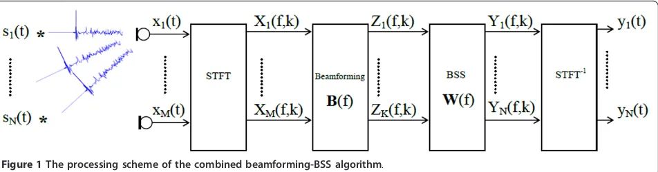
The separation matrix F(f) is estimated using a two-step blind separation algorithm: a fixed beamforming preprocessing step and a BSS step (cf. Figure 1). F(f) is written as the combination of the results of those two steps:

Maazaouiet al.EURASIP Journal on Advances in Signal Processing2012,2012:58 http://asp.eurasipjournals.com/content/2012/1/58

(3)

F(f) =W(f)B(f) (4)

whereW(f) is the separation matrix estimated using a sparsity criterion andB(f) is a fixed beamforming filter. More details are presented in the following subsections (cf. Algorithm 1).

2.1 Beamforming preprocessing

The role of the beamformer is essentially to reduce the reverberation and the interferences coming from direc-tions other than the looked up ones. Once the rever-beration is reduced, Equation (2) is better satisfied which leads to an improved BSS quality.

We consider{B(f)}₁_≤_f_≤Nf

2 +1

a set of fixed

beamform-ing filters of sizeK×M, whereKis the number of the

desired beams, K ≥ N. Those filters are calculated

beforehand (before the beginning of the processing) and used in the beamforming preprocessing step (cf. Section

3). The outputs of the beamformers at each frequencyf

are:

Z(f,k) =B(f)X(f,k) (5)

2.2 Blind source separation

The BSS step consists in estimating a separation matrix

W(f) that leads to separated sources at each frequency binf. The separation matrixW(f) is estimated by mini-mizing, with respect toW(f), a cost function ψbased on a sparsity criterion, under a unit norm constraints for

W(f). The chosen optimization technique is the natural gradient (cf. Section 4). The separation matrix is esti-mated from the output signals of the beamformers Z(f,

k) and the estimated sources are then written as:

Y(f,k) =W(f)Z(f,k) (6)

3 Fixed beamforming using HRTF

In the case of robot audition, the geometry of the microphone array is fixed once for all. To build the fixed beamformers, we need to determine the“desired”

steering directions and the characteristics of the beam pattern (the beamwidth, the amplitude of the sidelobes and the position of nulls). The beamformers are esti-mated only once for all scenarii using these spatial information and independently of the measured mixture in the sensors.

The least-square (LS) technique is used [6] to estimate the beamformer filters that will achieve the desired beam pattern according to a desired direction response. To accomplish this beamformers estimation, we need to calculate the steering vectors which represent the phase delays of a plane wave evaluated at the microphone array elements.

In the free field, the steering vector of anM elements array at a frequencyf and for a steering directionθ is known. For example, for a linear array, we have:

a(f,θ) =

1,e−j2πfdcsinθ_{, ...,}_e−j2πf d

c(M−1) sinθ

T

(7)

wheredis the distance between two sensors and cis

the speed of sound.

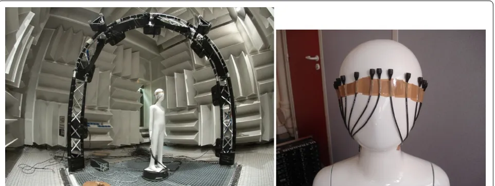
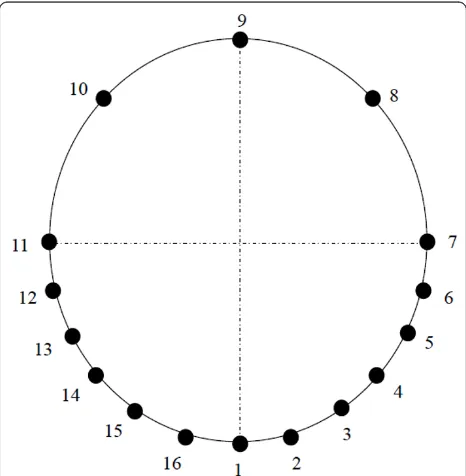
In the case of robot audition, the microphones are often fixed in the head of the robot (cf. Figure 2). The free field model of the steering vectors presented in Equation (7) does not take into account the influence of the head on the surrounding acoustic fields, and in this case, the microphone array manifold is not modeled (unknown).

For a human hearing, there is a spectral filtering of the sound source by the head and the pinna, and thus a transfer function between the source and each ear is defined and refered to as: the HRTF. The HRTF takes into account the interaural time differenceb(ITD), the interaural intensity differencec (IID) and the shape of the head and the pinna. It defines how a sound emitted from a specific location and altered by the head and the pinna is received at an ear. The notion of HRTF remains the same if we replace the human head by a dummy head and the ears by two microphones. We extend the usual concept of binaural HRTF to the con-text of robot audition where the humanoid is equipped

(4)

with a microphone array. In our case, a HRTF hm(f,θ) at frequencyfcharacterizes how a signal emitted from a specific directionθis received at themth sensor fixed in a head.

We propose to use the HRTFs as steering vectors for the beamformer filters calculation (cf. figure 3) and replace the unknown array manifold by a discrete

distri-bution of HRTFs on a group of NS a priori chosen

steering directions =θ1, ...,θNS

. The HRTFs are measured in an anechoïc room as explained in Section 5.

Let hm (f,θ) be the HRTF at frequency f from the

emission point located at θ to the mth sensor. The

steering vector is then:

a(f,θ) =h1(f,θ), ...,hM(f,θ)

T

(8)

Figure 2The dummy in the anechoïc room (left) and the microphone array of 16 sensors (right).

Figure 3Example of a beam pattern using HRTFs forθi= 50° (in dB).

(5)

Given Equation (8), one can express the normalized LS beamformer for a desired directionθias [6]:

b(f,θi) =

R−_aa1(f)a(f,θi)

aH₍_f_,_θ

i)R−aa1(f)a(f,θi)

(9)

where Raa(f) = _N1_S _θ_∈a(f,θ)aH(f,θ). Given K

desired steering directions θ1,...,θK, the beamforming matrixB(f) is:

B(f) =b(f,θ1), ...,b(f,θK)

T

(10)

In the following, we present the different configura-tions of the combined beamforming-BSS algorithm.

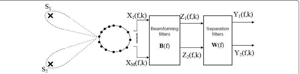
3.1 Beamforming with known DOA

If the direction-of-arrivals (DOAs) of the sources are

known a priori, mainly by a source localization

method, the beamforming filters are estimated using this spatial information of the sources location (cf. Fig-ure 4). Therefore, the desired directions are the DOAs of the sources and we select the corresponding HRTFs to build the desired response vectors a(f,θ). This is an ideal method to compare our results with. Indeed, we consider that source localization is beyond the scope of this article (in [7] where the beamforming with known DOAs was proposed for a circular microphone array, the authors have assumed that the DOAs are knowna priori).

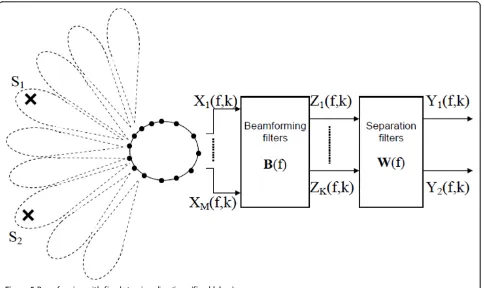
3.2 Beamforming with fixed DOA

Estimating the DOAs of the sources to build the beam-formers is time consuming and not always accurate in

the reverberant environments. So we propose to buildK

fixed beams with arbitrary desired directions chosen such as they cover all the useful space directions (cf. Fig-ure 5). We use the output of all the beamformers directly in the BSS algorithm. In this case, we still have

an overdetermined separation problem with Nsources

andKmixtures.

3.3 Beamforming with beams selection

In this configuration, we still haveKfixed beams with arbitrary desired directions, but we are not going to use all the outputs of those beamformers (cf. figure 6). We select theNbeamformer outputs with the highest energy, corresponding to the beams that are the closest to the sources (we suppose that the energies of the sources are quite close to each other). In this case, after

beamform-ing, we are in a determined separation problem withN

sources andK=Nmixtures (cf. Algorithm 2).

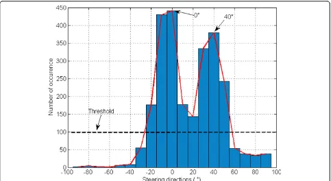
Fixed beamforming with beams selection can be derived and used for the source number as well as a rough DOAs estimation. We fix a maximum number of sourcesNmax <K. In each frequency bin, after the

beam-forming filtering (5), we select theNmaxbeams with the

highest energies (instead of selectingNbeams as in the previous paragraph). Then, we build over all the selected steering directions a histogram that corresponds to their

overall number of occurrence (cf. Figure 7). After a

thresholding, we select the beams corresponding to the peaks (a peak corresponds to a local maximum point associated to the number of selected beams over all the frequencies). The filters that correspond to those beams are our final beamforming filters, the number of peaks correspond to the number of sources and the corre-sponding steering directions provide us with a rough estimation of the DOAs.

4 BSS using sparsity criterion

In the BSS step, we estimate the separation matrixW(f)

by minimizing, with respect to the separation matrix W

(f), a cost function ψ based on a sparsity criterion, under a unit norm constraint forW(f):

min

W ψ(W(f)) such that W(f)= 1 (11)

The optimization technique used to update the separation matrix W(f) is the natural gradient. Section 4.1 summarizes the natural gradient algorithm [11], Sec-tion 4.2 shows how we use this optimizaSec-tion algorithm in our cost function.

(6)

4.1 Natural gradient algorithm

The natural gradient is an optimization method pro-posed by Amari et al. [11]. In this modified gradient search method, the standard gradient search direction is altered according to the local Riemannien structure of

the parameter space. This guarantees the invariance of the natural gradient search direction to the statistical relationship between the parameters of the model and leads to a statistically efficient learning performance [12].

Figure 5Beamforming with fixed steering directions (fixed lobes).

Figure 6Beamforming with fixed steering directions and beams selection. Maazaouiet al.EURASIP Journal on Advances in Signal Processing2012,2012:58 http://asp.eurasipjournals.com/content/2012/1/58

(7)

Assume that we want to update a separation matrix

W according to a loss function ψ (W). The gradient

update of this matrix is given by:

Wt+1=Wt−μ∇ψ(Wt) (12)

where ∇ψ(W) is the gradient of the function ψ(W) andtrefers to the iteration (or time) index. From [12],

the natural gradient of a loss function ψ (W), noted

˜∇ψ(W), is given by:

˜∇ψ(W) =∇ψ(W)WHW (13) The natural gradient update of the separation matrix

Wis then:

Wt+1=Wt−μ∇ψ(Wt)WHt Wt (14)

4.2 Sparsity separation criterion

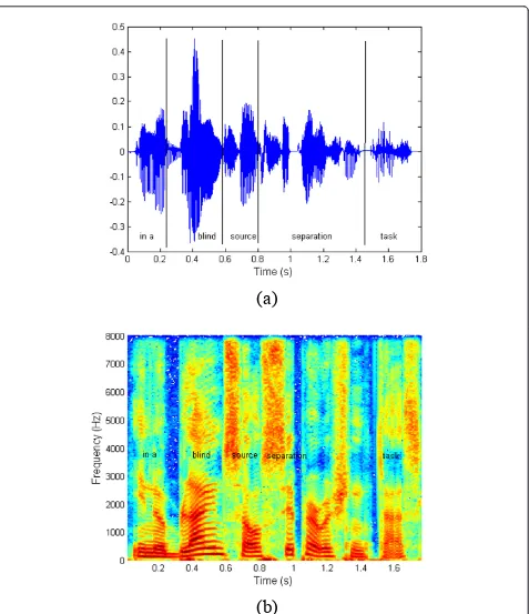
Speech signal is known to be sparse in the time-fre-quency domain: the number of time-fretime-fre-quency points where the speech signal is active (i.e., of non negligeable energy) is small comparing to the total number of time-frequency points (cf. Figure 8).

We consider a separation criterion based on the spar-sity of the signals in the time-frequency domain. For

every frequency bin, we look for a separation matrix W

(f) that leads to the sparsest estimated sources Y(f,:) = [Y(f,1),...,Y(f,NT)].

In the same manner, we define the mixture matrix in each frequency binX(f,:) = [X(f,1),...,X(f,NT)].

To measure the sparsity of a signal, the l1norm is the

most used sparsity measure thanks to its convexity [13]. The smaller is the l1 norm of a signal, the sparser it is.

However, thel1 norm is not the only measure of

spar-sity [13]. We presented recently a parameterized lp

norm algorithm for BSS, where we made the sparsity constraint harder through the iterations of the optimiza-tion process [14]. In this article, we use the l1 norm to

measure the sparsity of signalY(f,:), and hence the cost function is:

ψ(W(f)) =

N

i=1

NT

k=1

Yi(f,k) (15)

To have the sparsest estimated sources, we should

minimize ψ(W(f)) and we use the natural gradient

search technique to find the optimum separation matrix

W(f):

Wt+1(f) =Wt(f)−μ∇ψ(Wt(f))WHt (f)Wt(f) (16)

The differential ofψ(W(f)) is:

dψ(W(f)) =f(Y(f, :))dYH(f, :) (17) where f(Y(f,:)) = sign(Y(f,:)) is a matrix with the same size asY(f,:) in which the (i, j)th entry is sign(Yi(f, j)).d

(8)

(a)

(b)

Figure 8Sparsity of the speech signal in the time-frequency domain comparing to the time domain.(a)Speech sentence in the time domain(b)Time-frequency representation of the speech sentence

(9)

Thus, the gradient ofψ(W) is expressed as:

∇ψ(W(f)) =f(Y(f, :))XH(f, :) (18) which gives the expression of the natural gradient of

ψ(Wt(f)):

˜∇ψ(Wt(f)) =∇ψ(Wt(f))WHt (f)Wt(f)

=f(Yt(f, :))YHt (f, :)Wt(f)

(19)

The update equation of Wt(f) for a frequency binfis then:

Wt+1(f) =Wt(f)−μGt(f)Wt(f) (20)

withGt(f) =f(Yt(f, :))YHt (f, :)..

The convergence of the natural gradient is condi-tioned both by the initial coefficients W0 (f) of the separation matrix and the step size of the update and it is quite difficult to choose the parameters that allow fast convergence without risking divergence. Douglas and Gupta [15] proposed to impose a scaling constraint to the separation matrixWt(f) to maintain a constant gra-dient magnitude along the algorithm iterations. They assert that with this scaling and a fixed step size μ, the algorithm has fast convergence and excellent perfor-mance independently of the magnitude ofX(f,:) andW0

(f). Applying this scaling constraint, our update function becomes:

Wt+1(f) =ct(f)Wt(f)−μc2t(f)Gt(f)Wt(f) (21)

withct(f) =

1 1 N N i=1 N j=1g

ij t(f)

and gij_t(f) =Gt(f)

ij.

4.3 Initialization

When we are in an overdetermined case, we use a whitening process for the initialization of the separation matrixW0. The whitening is an important preprocessing in an overdetermined BSS algorithm as it allows to focus the energy of the received signals in the useful signal space. The separation matrix is initialized as follow:

W0=

D−_M1EH_:_M

whereDmis a matrix containing the firstM rows and

M columns of the matrixD andE:M is the matrix

con-taining the firstM columns of the matrixE. D and E

are respectively the diagonal matrix and the unitary matrix of the singular value decomposition of the auto-correlation matrix of the received dataX(f,:) or the fil-tered data after beamformingZ(f,:).

If we are in a determined case, in particular when we select the beams with the highest energy after the beam-forming filtering or when the steering directions

correspond to the direction of arrivals of the sources, the initialization of the separation matrix is done with the identity matrix:

W0=IN

5 Experimental results

5.1 Experimental database

To evaluate the proposed BSS techniques, we built two databases: a HRTFs database and a speech database. 5.1.1 HRTF database

We recorded the HRTF database in the anechoic room

of Telecom ParisTech (cf. Figure 2) using the Golay

codes process [16]. As we are in a robot audition con-text, we model the future robot by a child size dummy (1m20) for the sound acquisition process, with 16 sen-sors fixed in its head (cf. Figure 9).

We measured 504 HRTF for each microphone as fol-low:

•72 azimuth angles from 0° to 355° with a 5° step

•7 elevation angles: -40°, -27°, 0°, 20°, 45°, 60° and 90°

To measure the HRTFs, the dummy was fixed on a turntable in the center of the loudspeaker arc in the anechoic room (cf. Figure 2). For each azimuth angle, a sequence of complementary Golay codes is emitted sequentially from each loudspeaker (this is to vary the elevation) and recorded with the 16 sensors array.

(10)

This operation was repeated for all the azimuth angles. The Golay complementary sequences have the useful property that their autocorrelation functions have complementary sidelobes: the sum of the auto-correlation sequences is exactly zero everywhere except at the origin. Using this property and the recorded complementary Golay codes, the HRTF are calculated as in [16].

Details about the experimental process of HRTF cal-culation as well as the HRTF databases at the sampling

frequencies of 48 and 16 KHz are available at http://

www.tsi.telecom-paristech.fr/aao/?p=347. 5.1.2 Test database

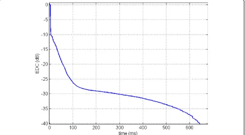
The test signals were recorded in a moderately

reverber-ant room where the reverberation time is RT30 = 300

ms (cf. Figure 10). Figure 11 shows the different posi-tions of the sources in the room. We chose to evaluate the proposed algorithm on a separation of two sources: the first source is always the one placed at 0° and the second source is chosen from 20° to 90°.

The output signals x(t) are the convolutions of 40 pairs of speech sources (male and female speaking French and English) by two of the impulse responses {h (l)}0≤l≤Lmeasured for the direction of arrivals presented in Figure 11.

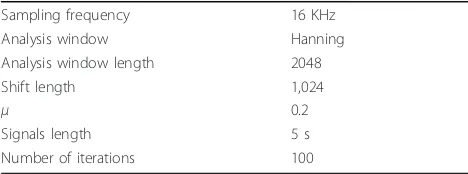
The characteristics of the signals and the BSS algo-rithms are summarized in Table 1.

5.2 Evaluation results

In this section, we evaluate different configurations of the presented algorithme:

(1) The beamforming stage only: beamforming of 37 lobes from -90° to 90° with a step angle of 5° (BF[5°]) (2) The BSS algorithm only

(a) with minimization of thel1 norm (BSS-l1)

(b) with ICA from [15] (ICA)

(3) The two-stage algorithm, BSS and the beamform-ing preprocessbeamform-ing:

(a) beamforming of Nlobes in the DOA of the

sources (BF[DOA]+BSS-l1)

(b) beamforming of 7 lobes from -90° to 90° with a step angle of 30° (BF[30°]+BSS-l1 when the l1

norm minimization is used in the BSS step and BF[30°]+ICA when ICA is used in the BSS step) (c) beamforming of 13 lobes from -90° to 90° with a step angle of 15° (BF[15°]+BSS-l1)

(d) beamforming of 19 lobes from -90° to 90° with a step angle of 10° (BF[10°]+BSS-l1)

(e) beamforming of 37 lobes from -90° to 90° with a step angle of 5° (BF[5°] +BSS-l1)

(f) beamforming of 7 lobes from -90° to 90° with a step angle of 30° with selection of theNbeams containing the highest energy before proceeding the BSS (BF[30°]+BS +BSS-l1)

Figure 10Energy decay curve of the room used for the reverberant recording. Maazaouiet al.EURASIP Journal on Advances in Signal Processing2012,2012:58 http://asp.eurasipjournals.com/content/2012/1/58

(11)

(g) beamforming of 37 lobes from -90° to 90°

with a step angle of 5° with selection of the N

beams containing the highest energy before pro-ceeding the BSS (BF[5°]+BS +BSS-l1)

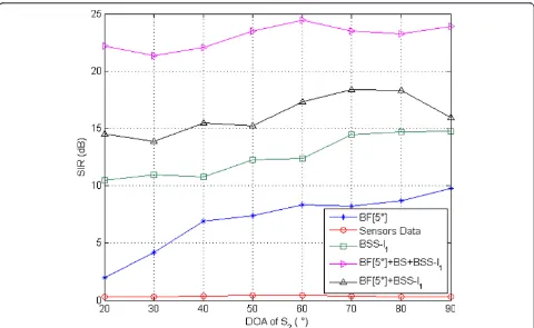
We evaluate the proposed two-stage algorithm by the signal-to-interference ratio (SIR) and the signal-to-dis-tortion ratio (SDR) estimated using the BSS-eval toolbox [17]. All the presented curves are the average result of the 40 pairs of speech.

5.2.1 Influence of the beamforming preprocessing

Figures 12 and 13 show that the SIR and SDR of the two-stage algorithm with the fixed beamforming prepro-cessing BF[5°] +BSS-l1 and BF[30°]+ BSS-l1 are better

than the SIR and SDR of the separation algorithm with

l1 norm alone BSS-l1and much better than the ones we

obtain by the fixed beamforming BF[5°] only. The SIR and SDR of the received signals in microphones 1 and 2 (labeled assensors datain the figures) is taken as refer-ence to illustrate the performance gain of our method. However this increase in the SIR and SDR by the fixed beamforming preprocessing is limited and do not reach the performance of the beamforming preprocessing with

known DOA BF[DOA]+BSS-l1 as shown in Figures 14

and 15. But we can overcome this limitation by the beam selection as shown in the sequel.

Figures 16 and 17 show the SIR and SDR obtained with different inter-beam angle of the beamforming pre-processing, the steering directions vary from -90° to 90°: beamforming with 7 beams with a step angle of 30° (BF

[30°] +BSS-l1), beamforming of 13 beams with a step

Figure 11The position of the sources and their directions of arrival in the reverberant room.

Table 1 Parameters of the blind source separation algorithms

Sampling frequency 16 KHz

Analysis window Hanning

Analysis window length 2048

Shift length 1,024

μ 0.2

Signals length 5 s

(12)

angle of 15° (BF[15°]+ BSS-l1), beamforming of 19

beams with a step angle of 10° (BF[10°]+BSS-l1) and

beamforming with 37 beams with a step angle of 5°. The results show that when we increase the number of the beams, the SIR and especially the SDR increases. For BF[15°]+BSS-l1, BF[10°] +BSS-l1 and BF[5°]+BSS-l1,

the beamforming preprocessing increases the SDR of the estimated sources comparing with the single stage

BSS-l1 algorithm. The SIR with a beamforming

prepro-cessing is also better than the single stage BSS-l1

algo-rithm, and this for all the tested configurations of the fixed steering direction beamforming prepossessing. Influence of the beams selection

As we can observe from Figures 12, 13, 14, and 15, the beamforming preprocessing with beams selection (BF [30°] +BS+ BSS-l1 and BF[5°]+BS+BSS-l1) and the

beam-forming preprocessing with known direction of arrivals (BF[DOA]+BSS-l1) have close results in terms of SIR (cf.

Figures 12 and 14) and SDR (cf. Figures 13 and 15).

However, if we are in a reverberant environment where the direction of arrivals can not be estimated accurately, the beamforming preprocessing with beams selection would be a good solution to improve the SIR and the SDR of the estimated sources comparing to the use of the BSS algorithm only (BSS-l1).

Comparing BF[5°]+BS +BSS-l1 in Figure 12 and BF

[30°] +BS+ BSS-l1 in Figure 14 show that the impact of

the inter-beam angle is quite weak with respect to the separation gain. However, the beamforming preproces-sing with beams selection of 5° inter-beam angle step allows us to estimate correctly the DOA of the sources with a step of 5° as shown in Figure 18. The latter represents the selected beam directions for all consid-ered experiments (i.e., the 40 experiments) and for dif-ferent source locations.

5.2.2 Comparison between BSS-l1and ICA

Independent component analysis and thel1norm

mini-mization have quite close results with or without the preprocessing step. However, we believe that replacing BSS-l1 by BSS-lp with p < 1 or with varying p value might lead to a significant improvement of the separa-tion quality. This observasepara-tion is based on the prelimin-ary results we obtained in [14] and would be the focus of future investigations.

5.2.3 Convergence analysis

We procceed to the analysis of the convergence of the proposed algorithm by observing the convergence rates through the iterations and for the considered DOA (cf. Figure 19). Each curve represents the average of cost function (15) averaged for all the frequencies. As we can

Figure 12SIR comparison in a real environment: source 1° is at 0° and source 2 varies from 20° to 90°–effect of the beamforming preprocessing on the SIR of the estimated sources.

(13)

Figure 13SDR comparison in a real environment: source 1 is at 0° and source 2 varies from 20° to 90°–effect of the beamforming preprocessing on the SDR of the estimated sources.

(14)

Figure 15SDR comparison in a real environment: source 1 is at 0° and source 2 varies from 20° to 90°.

Figure 16SIR of different configuration of the beamforming preprocessing with fixed steering direction: inter-beams angles are 30°, 15°, 10°, and 5°, respectively.

(15)

Figure 17SDR of different configuration of the beamforming preprocessing with fixed steering direction: inter-beams angles are 30°, 15°, 10°, and 5°, respectively.

(16)

see in Figure 19b, our iterative algorithm converges quite quickly (typically 10 to 20 iterations) towards its steady state. We notice also that the convergence rate of the proposed two stage method with beam selection is

better than the convergence of BSS-l1. Indded, in this

context, the separation algorithm BSS-l1 converges to its

steady state after 30 to 40 iterations. Moreover, the cost function of the two stage algorithm reaches lower values

(a)

(b)

Figure 19Convergence rates: the value of the cost function through the iterations and for different DOA. (a) BSS-l1(b) BF[5°]+BS+BSS-l1

(17)

than the separation algorithm only and thus, the beam-forming preprocessing helps for better convergence.

6 Conclusion

In this article, we present a two-stage BSS algorithm for robot audition. The first stage is a preprocessing step with fixed beamforming. To deal with the effect of the head of the robot in the acoustic near field and model the manifold of the sensors array, we used HRTFs as steering vectors in the beamformers estimation step. The second stage is a BSS algorithm exploiting the spar-sity of the sources in the time-frequency domain.

We tested different configurations of this algorithm with steering directions of the beams equal to the direc-tion of arrivals of the sources and with fixed steering directions. We also varied the step angle between the beams. The beamforming preprocessing improves the separation performance as it reduces the reverberation and noise effects. The maximum gain is obtained when we select the beams with the highest energies and use the corresponding filters as beamformers or when the sources DOAs are known. The beamforming preproces-sing with fixed steering directions has also good perfor-mance and does not use an estimation of the DOAs or beam selection, which represent a gain in the processing time. Using the 5° step beamforming preprocessing with beams selection, we can also have a rough estimation of the direction of arrivals of the sources.

Endnotes

a

Romeo project: http://www.projetromeo.com.bThe ITD

is the difference in arrival times of a sound wavefront at the left and right ears.cThe IID is the amplitude differ-ence of a sound that reaches the right and left ears.dFor a complex number z,sign(z) = _|z_z_|. eThe names of the algorithms that we are going to use in the legends of the figures are between brackets.

Algorithm 1Combined beamforming and BSS algo-rithm

1.Input:

(a) The output of the microphone array x = [x

(t1),...,x(tT)]

(b) The beamforming pre-calculated filters

{B(f)} 1≤f≤Nf

2+1

2.{X(f,k)}1≤f≤Nf,1≤k≤NT =STFT(x) 3. for each frequency bin f

(a) beamforming preprocessing step:Z (f,:) =B (f)X(f,:)

(b) initialization step:W(f) =W0 (f) (c)Y0 (f,:) =W0(f)Z(f,:)

(d) for each iterationt:

blind source separation step to estimateW(f)

4. Permutation problem solving

5. Output: the estimated sources

y= ISTFT{Y(f,k)}₁_≤_f_≤_N_f_,1_≤_k_≤_N_K Algorithm 2Beams selection algorithm

1. SelectedBeams = Ø 2. for each frequency binf:

(a) FormKbeams (beamformer outputs)Z(f,:) =

B(f)X(f,:),Z(f,:) = [z1(f,:),...,zK(f,:)]T

(b) Compute the energy of the beamformer out-puts: E(f) = [e1(f),...,eK(f)] with ei(f) = _N1_T _kN₌₁T zi(f,k)

2

(c) Decreasing order sort of E(f), Beams are the beams corresponding to the sorted energies: Beams =sort(E(f))

(d) Select theNhighest energies, the indexes are stored inB.

(e) SelectedBeams = SelectedBeams∪B

3. Compute the frequency of appearance of each beam and store the occurrences inI.

4. Select theNbeams with the highest occurrence

Acknowledgements

This work is funded by the Ile-de-France region, the General Directorate for Competitiveness, Industry and Services (DGCIS) and the City of Paris, as a part of the ROMEO project.

Competing interests

The authors declare that they have no competing interests.

Received: 15 June 2011 Accepted: 6 March 2012 Published: 6 March 2012

References

1. Pierre Comon, Christian Jutten,Handbook of Blind Source Separation Independent Component Analysis and Applications, (Elsevier, 2010) 2. Y Tamai, Y Sasaki, S Kagami, H Mizoguchi,_“Three ring microphone array for

3d sound localization and separation for mobile robot audition,”.IEEE/RSJ International Conference on Intelligent Robots and Systems4172–4177 (Aug 2005)

3. S Yamamoto, K Nakadai, M Nakano, H Tsujino, J-M Valin, K Komatani, T Ogata, HG Okuno,_“Design and implementation of a robot audition system for automatic speech recognition of simultaneous speech,”.IEEE Workshop on Automatic Speech Recognition Understanding111_–116 (2007) 4. H Nakajima, K Nakadai, Y Hasegawa, H Tsujino,“High performance sound

source separation adaptable to environmental changes for robot audition,_”. IEEE/RSJ International Conference on Intelligent Robots and Systems 2165_–2171 (Sept 2008)

5. H Saruwatari, Y Mori, T Takatani, S Ukai, K Shikano, T Hiekata, T Morita, “Two-stage blind source separation based on ica and binary masking for real-time robot audition system,”.IEEE/RSJ International Conference on Intelligent Robots and Systems2303–2308 (2005)

6. Jacob Benesty, Jingdong Chen, Yiteng Huang,Microphone Array Signal Processing Chapter 3: Conventional beamforming techniques, 1st edn. (Springer, 2008)

(18)

8. Pierre Comon,“Independent component analysis, a new concept?,”Signal Processing(1994)

9. H Saruwatari, S Kurita, K Takeda, F Itakura, T Nishikawa, K Shikano,“Blind source separation combining independent component analysis and beamforming,”.EURASIP Journal on Applied Signal Processing1135–1146 (2003)

10. Wang Weihua, Huang Fenggang,“Improved method for solving permutation problem of frequency domain blind source separation,_”6th IEEE International Conference on Industrial Informatics703–706 (July 2008) 11. S Amari, A Cichocki, HH Yang,“A new learning algorithm for blind signal separation,”Advances in Neural Information Processing Systems757–763 (1996)

12. Shun-Ichi Amari,_“Natural gradient works efficiently in learning,_”Neural Computation.10, 251–276 (1998). doi:10.1162/089976698300017746 13. Hurley Niall, Rickard Scott,_“Comparing measures of sparsity,_”IEEE Workshop

on Machine Learning for Signal Processing.55, 4723–4741 (October 2009) 14. M Maazaoui, Y Grenier, K Abed-Meraim,_“Frequency domain blind source separation for robot audition using a parameterized sparsity criterion,”19th European Signal Processing Conference EUSIPCO(2011)

15. SC Douglas, M Gupta,“Scaled natural gradient algorithms for instantaneous and convolutive blind source separation,”.IEEE International Conference on Acoustics, Speech and Signal Processing.2, 637_–640 (Apr 2007)

16. S Foster,“Impulse response measurement using golay codes,”IEEE International Conference on Acoustics, Speech, and Signal Processing, ICASSP ‘86.11, 929–932 (Apr 1986)

17. E Vincent, R Gribonval, C Fevotte,_“Performance measurement in blind audio source separation,”IEEE Transactions on Audio, Speech, and Language Processing.14, 1462_–1469 (July 2006)

doi:10.1186/1687-6180-2012-58

Cite this article as:Maazaouiet al.:Blind source separation for robot

audition using fixed HRTF beamforming.EURASIP Journal on Advances in Signal Processing20122012:58.