Unsupervised Model Adaptation using Information Theoretic Criterion

Unsupervised Model Adaptation using Information-Theoretic Criterion

Ariya Rastrow1, Frederick Jelinek1, Abhinav Sethy2 and Bhuvana Ramabhadran2 1_{Human Language Technology Center of Excellence, and}

Center for Language and Speech Processing, Johns Hopkins University {ariya, jelinek}@jhu.edu

2_{IBM T.J. Watson Research Center, Yorktown Heights, NY, USA}

{asethy, bhuvana}@us.ibm.com

Abstract

In this paper we propose a novel general framework for unsupervised model adapta-tion. Our method is based on entropy which has been used previously as a regularizer in semi-supervised learning. This technique in-cludes another term which measures the sta-bility of posteriors w.r.t model parameters, in addition to conditional entropy. The idea is to use parameters which result in both low con-ditional entropy and also stable decision rules. As an application, we demonstrate how this framework can be used for adjusting language model interpolation weight for speech recog-nition task to adapt from Broadcast news data to MIT lecture data. We show how the new technique can obtain comparable performance to completely supervised estimation of inter-polation parameters.

1 Introduction

All statistical and machine learning techniques for classification, in principle, work under the assump-tion that

1. A reasonable amount of training data is avail-able.

2. Training data and test data are drawn from the same underlying distribution.

In fact, the success of statistical models is cru-cially dependent on training data. Unfortunately, the latter assumption is not fulfilled in many appli-cations. Therefore, model adaptation is necessary when training data is not matched (not drawn from

same distribution) with test data. It is often the case where we have plenty of labeled data for one specific domain/genre (source domain) and little amount of labeled data (or no labeled data at all) for the de-sired domain/genre (target domain). Model adapta-tion techniques are commonly used to address this problem. Model adaptation starts with trained mod-els (trained on source domain with rich amount of la-beled data) and then modify them using the available labeled data from target domain (or instead unla-beled data). A survey on different methods of model adaptation can be found in (Jiang, 2008).

Information regularization framework has been previously proposed in literature to control the la-bel conditional probabilities via input distribution (Szummer and Jaakkola, 2003). The idea is that la-bels should not change too much in dense regions of the input distribution. The authors use the mu-tual information between input features and labels as a measure of label complexity. Another framework previously suggested is to use label entropy (condi-tional entropy) on unlabeled data as a regularizer to Maximum Likelihood (ML) training on labeled data (Grandvalet and Bengio, 2004).

Availability of resources for the target domain

cat-egorizes these techniques into either supervised or

unsupervised. In this paper we propose a general framework for unsupervised adaptation using Shan-non entropy and stability of entropy. The assump-tion is that in-domain and out-of-domain distribu-tions are not too different such that one can improve the performance of initial models on in-domain data by little adjustment of initial decision boundaries (learned on out-of-domain data).

2 Conditional Entropy based Adaptation

In this section, conditional entropy and its relation to classifier performance are first described. Next, we introduce our proposed objective function for do-main adaptation.

2.1 Conditional Entropy

Considering the classification problem whereXand

Yare the input features and the corresponding class

labels respectively, the conditional entropy is a mea-sure of the class overlap and is calculated as follows

H(Y|X) =EX[H(Y|X=x)] =

− Z

p(x) X

y

p(y|x) logp(y|x)

!

dx (1)

Through Fano’s Inequalitytheorem, one can see

how conditional entropy is related to classification performance.

Theorem 1 (Fano’s Inequality) Suppose

Pe = P{Yˆ 6= Y} where Yˆ = g(X) are the

assigned labels for the data points, based on the classification rule. Then

Pe≥

H(Y|X)−1

log(|Y| −1)

where Y is the number of possible classes and

H(Y|X) is the conditional entropy with respect to true distibution.

The proof to this theorem can be found in (Cover and

Thomas, 2006). This inequality indicates thatYcan

be estimated with low probability of error only if the

conditional entropyH(Y|X)is small.

Although the above theorem is useful in a sense that it connects the classification problem to Shan-non entropy, the true distributions are almost never

known to us1. In most classification methods, a

spe-cific model structure for the distributions is assumed and the task is to estimate the model parameters within the assumed model space. Given the model

1

In fact, Theorem 1 shows how relevant the input features are for the classification task by putting a lower bound on the best possible classifier performance. As the overlap between features from different classes increases, conditional entropy in-creases as well, thus lowering the performance of the best pos-sible classifier.

structure and parameters, one can modifyFano’s

In-equalityas follows,

Corollary 1

Pe(θ) =P{Yˆ 6=Y|θ} ≥

Hθ(Y|X)−1 log(|Y| −1)

(2)

where Pe(θ) is the classifier probability of error

given model parameters,θand

Hθ(Y|X) =

− Z

p(x) X

y

pθ(y|x) logpθ(y|x) !

dx

Here,Hθ(Y|X)is the conditional entropy imposed

by model parameters.

Eqn. 2 indicates the fact that models with low

conditional entropy are preferable. However, a low entropy model does not necessarily have good

per-formance (this will be reviewed later on)2

2.2 Objective Function

Minimization of conditional entropy as a framework in the classification task is not a new concept and has been tried by researchers. In fact, (Grandvalet and Bengio, 2004) use this along with the maxi-mum likelihood criterion in a semi-supervised set up such that parameters with both maximum like-lihood on labeled data and minimum conditional en-tropy on unlabeled data are chosen. By minimiz-ing the entropy, the method assumes a prior which prefers minimal class overlap. Entropy minimiza-tion is used in (Li et al., 2004) as an unsupervised non-parametric clustering method and is shown to

result in significant improvement overk-mean,

hier-archical clustering and etc.

These methods are all based on the fact that mod-els with low conditional entropy have their decision boundaries passing through low-density regions of

the input distribution,P(X). This is consistent with

the assumption that classes are well separated so that one can expect to take advantage of unlabeled exam-ples (Grandvalet and Bengio, 2004).

In many cases shifting from one domain to an-other domain, initial trained decision boundaries (on

out-of-domain data) result in high conditional en-tropy for the new domain, due to mismatch be-tween distributions. Therefore, there is a need to adjust model parameters such that decision bound-aries goes through low-density regions of the distri-bution. This motivates the idea of using minimum conditional entropy criterion for adapting to a new domain. At the same time, two domains are often close enough that one would expect that the optimal parameters for the new domain should not deviate too much from initial parameters. In order to formu-late the technique mentioned in the above paragraph,

let us define Θinit to be the initial model

parame-ters estimated on out-of-domain data (using labeled data). Assuming the availability of enough amount of unlabeled data for in-domain task, we try to min-imize the following objective function w.r.t the pa-rameters,

θnew = argmin

θ

Hθ(Y|X) +λ||θ−θinit||p

(3)

where||θ−θinit||p is anLpregularizer and tries to

prevent parameters from deviating too much from

their initial values3.

Once again the idea here is to adjust the param-eters (using unlabeled data) such that low-density separation between the classes is achieved. In the following section we will discuss the drawback of this objective function for adaptation in realistic sce-narios.

3 Issues with Minimum Entropy Criterion

It is discussed in Section 2.2 that the model param-eters are adapted such that a minimum conditional entropy is achieved. It was also discussed how this is related to finding decision boundaries through low-density regions of input distribution. However, the obvious assumption here is that the classes are well separated and there in fact exists low-density regions between classes which can be treated as boundaries. Although this is a suitable/ideal assumption for clas-sification, in most practical problems this assump-tion is not satisfied and often classes overlap. There-fore, we can not expect the conditional entropy to be

3_{The other reason for using a regularizer is to prevent trivial} solutions of minimum entropy criterion

convex in this situation and to achieve minimization w.r.t parameters (other than the trivial solutions).

Let us clarify this through an example. Consider

X to be generated by mixture of two 2-D

Gaus-sians (each with a particular mean and covariance matrix) where each Gaussian corresponds to a par-ticular class ( binary class situation) . Also in order to have linear decision boundaries, let the Gaussians have same covariance matrix and let the parameter

being estimated be the prior for class 1,P(Y = 1).

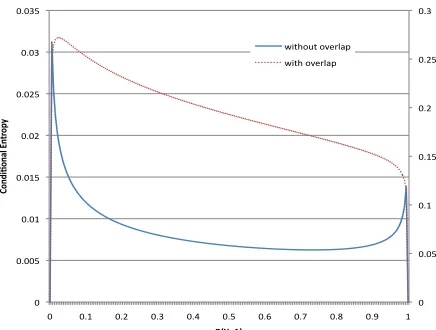
Fig. 1 shows two different situations with

over-lapping classes and non-overover-lapping classes. The left panel shows a distribution in which classes are well separated whereas the right panel corresponds to the situation where there is considerable overlap between classes. Clearly, in the later case there is no low-density region separating the classes. There-fore, as we change the parameter (here, the prior on

the classY = 1), there will not be any well defined

point with minimum entropy. This can be seen from Fig. 2 where model conditional entropy is plotted vs. class prior parameter for both cases. In the case of no-overlap between classes, entropy is a convex function w.r.t the parameter (excluding trivial

solu-tions which happens at P(Y = 1) = 0,1) and is

minimum atP(Y = 1) = 0.7which is the true prior

with which the data was generated.

We summarize issues with minimum entropy cri-terion and our proposed solutions as follows:

• Trivial solution: this happens when we put

de-cision boundaries such that both classes are considered as one class (this can be avoided us-ing the regularizer in Eqn. 3 and the assump-tion that initial models have a reasonable solu-tion, e.g. close to the optimal solution for new domain )

• Overlapped Classes: As it was discussed in

this section, if the overlap is considerable then the entropy will not be convex w.r.t to model

parameters. We will address this issue in

the next section by introducing the entropy-stability concept.

4 Entropy-Stability

ï3 ï2 ï1 0 1 2 3 4 5 6 7 ï4 ï2 0 2 4 6 8 10 X₁ X2

ï3 ï2 ï1 0 1 2 3 4 5 6 7

ï3 ï2 ï1 0 1 2 3 4 5 6 7 X1 X2

Figure 1: Mixture of two Gaussians and the corresponding Bayes decision boundary: (left) with no class overlap (right) with class overlap

0   0.05   0.1   0.15   0.2   0.25   0.3  

0   0.005   0.01   0.015   0.02   0.025   0.03   0.035  

0   0.1   0.2   0.3   0.4   0.5   0.6   0.7   0.8   0.9   1  

Co

nd

i&o

na

l  E

nt

ro

py

P(Y=1)  

without  overlap   with  overlap  

Figure 2: Condtional entropy vs. prior parameter,P(Y =

1)

situations where there is a considerable amount of overlap among classes. Assuming that class bound-aries happen in the regions close to the tail of class

distributions, we introduce the concept of

Entropy-Stability and show how it can be used to detect

boundary regions. DefineEntropy-Stabilityto be the

reciprocal of the following

∂Hθ(Y|X)

∂θ p = Z

p(x) ∂P

ypθ(y|x) logpθ(y|x) ∂θ dx p (4)

Recall: sinceθis a vector of parameters, ∂Hθ(Y|X)

∂θ

will be a vector and by using Lp norm

Entropy-stability will be a scalar.

The introduced concept basically measures the stability of label entropies w.r.t the model parame-ters. The idea is that we prefer models which not only have low-conditional entropy but also have sta-ble decision rules imposed by the model. Next, we show through the following theorem how Entropy-Stability measures the stability over posterior prob-abilities (decision rules) of the model.

Theorem 2

∂Hθ(Y|X)

∂θ p = Z

p(x) X

y

∂pθ(y|x)

∂θ logpθ(y|x)

! dx p

where the term inside the parenthesis is the weighted sum (by log-likelihood) over the gradient of poste-rior probabilities of labels for a given samplex

Proof The proof is straight forward and uses the fact

thatP∂pθ(y|x)

∂θ =

∂(P pθ(y|x))

∂θ = 0.

Using Theorem 2 and Eqn. 4, it should be clear how Entropy-Stability measures the expected sta-bility over the posterior probabilities of the model. A high value of

∂Hθ(Y|X)

∂θ

p implies models with

regions) we once again refer back to our mixture of Gaussians’ example. As the decision boundary moves from class specific regions to overlapped re-gions (by changing the parameter which is here class prior probability) we expect the entropy to continu-ously decrease (due to the assumption that the over-laps occur at the tail of class distributions). How-ever, as we get close to the overlapping regions the added data points from other class(es) will resist changes in the entropy. resulting in stability over the entropy until we enter the regions specific to other class(es).

In the following subsection we use this idea to propose a new objective function which can be used as an unsupervised adaptation method even for the case of input distribution with overlapping classes.

4.1 Better Objective Function

The idea here is to use the Entropy-Stability con-cept to accon-cept only regions which are close to the overlapped parts of the distribution (based on our assumption, these are valid regions for decision boundaries) and then using the minimum entropy criterion we find optimum solutions for our parame-ters inside these regions. Therefore, we modify Eqn. 3 such that it also includes the Entropy-Stability term

θnew = argmin

θ

Hθ(Y|X) +γ

∂Hθ(Y|X)

∂θ

p0

+ λ||θ−θinit||p

(5)

The parameter γ and λ can be tuned using small

amount of labeled data (Dev set).

5 Speech Recognition Task

In this section we will discuss how the proposed framework can be used in a speech recognition task.

In the speech recognition task, Y is the sequence

of words and X is the input speech signal. For a

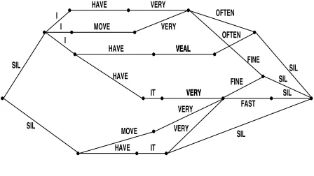
given speech signal, almost every word sequence is a possible output and therefore there is a need for a compact representation of output labels (words). For this, word graphs (Lattices) are generated dur-ing the recognition process. In fact, each lattice is an acyclic directed graph whose nodes correspond

to particular instants of time, and arcs (edges con-necting nodes) represent possible word hypotheses. Associated with each arc is an acoustic likelihood and language model likelihood scores. Fig. 3 shows

an example of recognition lattice4(for the purpose

of demonstration likelihood scores are not shown).L. Manguet al.: Finding Consensus in Speech Recognition 6

(a) Input lattice (“SIL” marks pauses)

SIL

SIL

SIL

SIL SIL

SIL VEAL

VERY HAVE

MOVE

HAVE

HAVE

IT

MOVE

HAVE IT

VERY

VERY

VEAL

VERY

VERY

VERY OFTEN

OFTEN

FINE

FINE

FAST I

I

I

(b) Multiple alignment (“-” marks deletions)

-

-I

MOVE

HAVE IT VEAL

VERY FINE

OFTEN

FAST

Figure 1:Sample recognition lattice and corresponding multiple alignment represented as confusion network.

alignment (which gives rise to the standard string edit distanceWE(W, R)) with a modified, multiple string alignment. The new approach incorporates all lattice hypotheses7_{into a single alignment, and word error between any two hypotheses}

is then computed according to that one alignment. The multiple alignment thus defines a new string edit distance, which we will callMWE(W, R). While the new alignment may in some cases overestimate the word error between two hypotheses, as we will show in Section 5 it gives very similar results in practice. The main benefit of the multiple alignment is that it allows us to extract the hypothesis with the smallest expected (modified) word error very efficiently. To see this, consider an example. Figure 1 shows a word lattice and the corre-sponding hypothesis alignment. Each word hypothesis is mapped to a position in the alignment (with deletions marked by “-”). The alignment also supports the computation ofword posterior probabilities. The posterior probability of a word hypothesis is the sum of the posterior probabilities of all lattice paths of which the word is a part. Given an alignment and posterior probabilities, it is easy to see that the hypothesis with the lowest expected word error is obtained by picking the word with the highest posterior at each position in the alignment. We call this theconsensus hypothesis.

7_{In practice we apply some pruning of the lattice to remove low probability word hypotheses}

(see Section 3.4).

Figure 3: Lattice Example

Since lattices contain all the likely hypotheses (unlikely hypotheses are pruned during recognition and will not be included in the lattice), conditional

entropy for any given input speech signal,x, can be

approximated by the conditional entropy of the lat-tice. That is,

Hθ(Y|X=xi) =Hθ(Y|Li)

whereLiis the corresponding decoded lattice (given

speech recognizer parameters) of utterancexi.

For the calculation of entropy we need to

know the distribution of X because Hθ(Y|X) =

EX[Hθ(Y|X=x)]and since this distribution is not

known to us, we useLaw of Large Numbersto

ap-proximate it by the empirical average

Hθ(Y|X)≈ − 1 N

N X

i=1 X

y∈Li

pθ(y|Li) logpθ(y|Li) (6)

Here N indicates the number of unlabeled

utter-ances for which we calculate the empirical value of conditional entropy. Similarly, expectation w.r.t in-put distribution in entropy-stability term is also ap-proximated by the empirical average of samples.

Since the number of paths (hypotheses) in the lat-tice is very large, it would be computationally infea-sible to compute the conditional entropy by enumer-ating all possible paths in the lattice and calculenumer-ating

4

Element hp, ri hp1, r1i⊗hp2, r2i hp1p2, p1r2+p2r1i hp1, r1i⊕hp2, r2i hp1+p2, r1+r2i

0 h0,0i

1 h1,0i

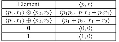
Table 1:First-Order (Expectation) semiring: Defining

multiplicationand sumoperations for first-order

semir-ings.

their corresponding posterior probabilities. Instead we use Finite-State Transducers (FST) to represent the hypothesis space (lattice). To calculate entropy and the gradient of entropy, the weights for the FST

are defined to be First- and Second-Ordersemirings

(Li and Eisner, 2009). The idea is to usesemirings

and their corresponding operations along with the forward-backward algorithm to calculate first- and second-order statistics to compute entropy and the gradient of entropy respectively. Assume we are in-terested in calculating the entropy of the lattice,

H(p) = −X d∈Li

p(d) Z log(

p(d) Z )

= logZ− 1

Z

X

d∈Li

p(d) logp(d)

= logZ− r¯

Z (7)

where Z is the total probability of all the paths in

the lattice (normalization factor). In order to do so,

we need to compute hZ,r¯i on the lattice. It can

be proved that if we define the first-order

semir-inghpe, pelogpei(peis the non-normalized score of

each arc in the lattice) as our FST weights and define semiring operations as in Table. 1, then applying the forward algorithm will result in the calculation of

hZ,r¯ias the weight (semiring weight) for the final

node.

The details for using Second-Ordersemiringsfor

calculating the gradient of entropy can be found

in (Li and Eisner, 2009). The same paper

de-scribes how to use the forward-backward algorithm to speed-up the this procedure.

6 Language Model Adaptation

Language Model Adaptation is crucial when the training data does not match the test data being de-coded. This is a frequent scenario for all Automatic

Speech Recognition (ASR) systems. The applica-tion domain very often contains named entities and N-gram sequences that are unique to the domain of

interest. For example, conversational speech has

a very different structure than class-room lectures. Linear Interpolation based methods are most com-monly used to adapt LMs to a new domain. As explained in (Bacchiani et al., 2003), linear inter-polation is a special case of Maximum A Posterior (MAP) estimation, where an N-gram LM is built on the adaptation data from the new domain and the two LMs are combined using:

p(wi|h) =λpB(wi|h) + (1−λ)pA(wi|h) 0≤λ≤1

where pB refers to out-of-domain (background)

models and pA is the adaptation (in-domain)

mod-els. Hereλis the interpolation weight.

Conventionally,λis calculated by optimizing

per-plexity (P P L) or Word Error Rate (W ER) on some

held-out data from target domain. Instead using

our proposed framework, we estimateλon enough

amount of unlabeled data from target domain. The idea is that resources on the new domain have al-ready been used to build domain specific models and it does not make sense to again use in-domain resources for estimating the interpolation weight. Since we are trying to just estimate one parameter and the performance of the interpolated model is bound by in-domain/out-of-domain models, there is no need to include a regularization term in Eqn. 5. Also

∂Hθ(Y|X)

∂θ

p =|

∂Hλ(Y|X)

∂λ |because we only

have one parameter. Therefore, interpolation weight will be chosen by the following criterion

ˆ

λ= argmin

0≤λ≤1

Hλ(Y|X) +γ|

∂Hλ(Y|X)

∂λ | (8)

For the purpose of estimating one parameterλ, we

useγ = 1in the above equation

7 Experimental Setup

are state-of-the-art discriminatively trained models and are the same ones used for all experiments pre-sented in this paper.

For LM adaptation experiments, the

out-of-domain LM (pB, Broadcast News LM) training

text consists of 335M words from the follow-ing broadcast news (BN) data sources (Chen et

al., 2006): 1996 CSR Hub4 Language Model

data, EARS BN03 closed captions, GALE Phase 2 Distillation GNG Evaluation Supplemental Mul-tilingual data, Hub4 acoustic model training tran-scripts, TDT4 closed captions, TDT4 newswire, and GALE Broadcast Conversations and GALE Broad-cast News. This language model is of order 4-gram

with Kneser-Ney smoothing and contains4.6M

n-grams based on a lexicon size of84K.

The second source of data is the MIT lectures data set (J. Glass, T. Hazen, S. Cyphers, I. Malioutov, D. Huynh, and R. Barzilay, 2007) . This serves as the target domain (in-domain) set for language model

adaptation experiments. This set is split into8hours

for in-domain LM building, another8hours served

as unlabeled data for interpolation weight estimation using criterion in Eqn. 8 (we refer to this as

unsuper-vised training data) and finally2.5hours Dev set for

estimating the interpolation weight w.r.tW ER

(su-pervised tuning) . The lattice entropy and gradient

of entropy w.r.tλare calculated on the unsupervised

training data set. The results are discussed in the next section.

8 Results

In order to optimize the interpolation weightλbased

on criterion in Eqn. 8, we devide[0,1]to 20

differ-ent points and evaluate the objective function (Eqn. 8) on those points. For this, we need to calculate entropy and gradient of the entropy on the decoded

lattices of the ASR system on8hours of MIT lecture

set which is used as an unlabeled training data. Fig. 4 shows the value of the objective function against different values of model parameters (interpolation

weight λ). As it can be seen from this figure just

considering the conditional entropy will result in a non-convex objective function whereas adding the entropy-stability term will make the objective func-tion convex. For the purpose of the evaluafunc-tion, we

show the results for estimatingλdirectly on the

tran-0 0.1 0.2 0.3 0.4 0.5 0.6 0.7 0.8 0.9 1

Model Entropy

Model Entropy+Entropy-Stability

BN-LM _λ MIT-LM

Figure 4: Objective function with and without including Entropy-Stability term vs. interpolation weight λon 8 hours MIT lecture unlabeled data

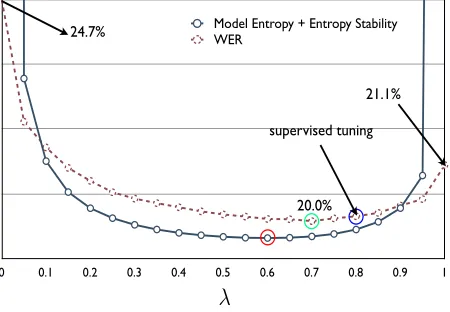
scription of the8hour MIT lecture data and compare

it to estimated value using our framework. The

re-sults are shown in Fig. 5. Usingλ= 0andλ= 1

theW ERs are24.7%and21.1%respectively.

Us-ing the new proposed objective function, the optimal

λis estimated to be0.6withW ERof20.1%(Red

circle on the figure). Estimatingλw.r.t8hour

train-ing data transcription (supervised adaptation) will

result inλ= 0.7(green circle) andW ERof20.0%.

Insteadλ= 0.8will be chosen by tuning the

inter-polation weight on2.5hour Dev set with

compara-bleW ERof20.1%. Also it is clear from the figure

that the new objective function can be used to

pre-dict theW ER trend w.r.t the interpolation weight

parameter.

0 0.1 0.2 0.3 0.4 0.5 0.6 0.7 0.8 0.9 1

Model Entropy + Entropy Stability WER

24.7%

20.0%

21.1%

supervised tuning

λ

Figure 5: Estimating λ based on W ER vs. the

information-theoretic criterion

unsuper-vised method results in the same performance as su-pervised adaptation in speech recognition task.

9 Conclusion and Future Work

In this paper we introduced the notion of entropy stability and presented a new criterion for unsu-pervised adaptation which combines conditional tropy minimization with entropy stability. The en-tropy stability criterion helps in selecting parameter settings which correspond to stable decision bound-aries. Entropy minimization on the other hand tends to push decision boundaries into sparse regions of the input distributions. We show that combining the two criterion helps to improve unsupervised pa-rameter adaptation in real world scenario where class conditional distributions show significant over-lap. Although conditional entropy has been previ-ously proposed as a regularizer, to our knowledge, the gradient of entropy (entropy-stability) has not been used previously in the literature. We presented experimental results where the proposed criterion clearly outperforms entropy minimization. For the speech recognition task presented in this paper, the proposed unsupervised scheme results in the same performance as the supervised technique.

As a future work, we plan to use the proposed criterion for adapting log-linear models used in Machine Translation, Conditional Random Fields (CRF) and other applications. We also plan to ex-pand linear interpolation Language Model scheme to include history specific (context dependent) weights.

Acknowledgments

The Authors want to thank Markus Dreyer and Zhifei Li for their insightful discussions and sugges-tions.

References

M. Bacchiani, B. Roark, and M. Saraclar. 2003.

Un-supervised language model adaptation. In Proc.

ICASSP, pages 224–227.

S. Chen, B. Kingsbury, L. Mangu, D. Povey, G. Saon, H. Soltau, and G. Zweig. 2006. Advances in speech transcription at IBM under the DARPA EARS pro-gram. IEEE Transactions on Audio, Speech and

Lan-guage Processing, pages 1596–1608.

Thomas M. Cover and Joy A. Thomas. 2006. Elements

of information theory. Wiley-Interscience, 3rd edition.

Yves Grandvalet and Yoshua Bengio. 2004.

Semi-supervised learning by entropy minimization. In

Advances in neural information processing systems

(NIPS), volume 17, pages 529–536.

J. Glass, T. Hazen, S. Cyphers, I. Malioutov, D. Huynh, and R. Barzilay. 2007. Recent progress in MIT spo-ken lecture processing project. InProc. Interspeech. Jing Jiang. 2008. A literature survey on domain

adapta-tion of statistical classifiers, March.

Zhifei Li and Jason Eisner. 2009. First- and second-order expectation semirings with applications to minimum-risk training on translation forests. InEMNLP. Haifeng Li, Keshu Zhang, and Tao Jiang. 2004.

Min-imum entropy clustering and applications to gene ex-pression analysis. InProceedings of IEEE

Computa-tional Systems Bioinformatics Conference, pages 142–

151.

Lidia Mangu, Eric Brill, and Andreas Stolcke. 1999. Finding consensus among words: Lattice-based word error minimization. InSixth European Conference on

Speech Communication and Technology.

M. Szummer and T. Jaakkola. 2003. Information regu-larization with partially labeled data. InAdvances in

Neural Information Processing Systems, pages 1049–