Volume 2006, Article ID 25431, Pages1–16 DOI 10.1155/ASP/2006/25431
Adaptive Subchip Multipath Resolving for
Wireless Location Systems
Nabil R. Yousef,1, 2Ali H. Sayed,1and Nima Khajehnouri1
1Electrical Engineering Department, University of California, Los Angeles, CA 90095-1594, USA 2Newport Media Inc., Lake Forest, CA 92630, USA
Received 31 May 2005; Revised 3 November 2005; Accepted 8 December 2005
Reliable positioning of cellular users in a mobile environment requires accurate resolving of overlapping multipath components. However, this task is difficult due to fast channel fading conditions and data ill-conditioning, which limit the performance of least-squares-based techniques. This paper develops two overlapping multipath resolving methods (adaptive and nonadaptive), and shows how the adaptive solution can be made robust to the above limitations by extracting and exploiting a priori information about the fading channel. Also the proposed techniques are extended when there are antenna arrays at the base station. Simulation results illustrate the performance of the proposed techniques.
Copyright © 2006 Hindawi Publishing Corporation. All rights reserved.
1. INTRODUCTION
Wireless propagation suffers frommultipathconditions. Un-der such conditions, the prompt ray may be succeeded by multipath components that arrive at the receiver within short delays. If this delay is smaller than the duration of the pulse shape used in the wireless system (i.e., the chip durationTc in CDMA systems), then the rays overlap. When this situa-tion occurs, it results in significant errors in the estimasitua-tion of the time and amplitude of arrival of the prompt ray.Figure 1
illustrates the combined impulse response of a two-ray chan-nel using a conventional pulse shape in a CDMA IS-95 sys-tem in two situations. In the second situation, where the pulses overlap, the location of the peak is obviously delayed relative to the location of the prompt ray. Such errors in the time-of-arrival are particularly damaging in wireless location applications (a topic of significant relevance nowadays—see, e.g., [1–18]). In these applications, small errors in the time-of-arrival can translate into many meters in terms of location inaccuracy.
There have been earlier studies in the literature on resolv-ing overlappresolv-ing multipath components (see, e.g., [19,20]). However, there are two sources of impairments that in-troduce significant errors into the resolution accuracy and which need special attention; these sources of error are par-ticularly relevant in the context of mobile-positioning sys-tems. The first impairment is due to the possibility of fast channel fading, which prohibits the use of long averaging intervals. This is because the estimation period in wireless
location applications can reach up to a few seconds, which may cause the channel between the transmitter and the re-ceiver to vary significantly during the estimation period, even for relatively slow channel variations. The second impair-ment is the possibility of noise enhanceimpair-ment, which occurs as a result of theill-conditioningof the data matrices involved in most least-squares-based solutions.
In this paper, we develop an adaptive technique for re-solving overlapping multipath components over fading channels for wireless location purposes. The technique is relatively robust to fast channel fading and data ill-condition-ing. The following are the main contributions of this work.
(1) We first describe a framework for overlapped mul-tipath resolving over fading channels via least squares. The framework will indicate why conventional least-squares tech-niques may fail for fading channels.
(2) We then point out the ill-conditioning problem that arises from using the pulse-shaping waveform deconvolution matrix. In order to avoid the possibility of noise enhance-ment as a result of this ill-conditioning, we show how to replace the least-squares operation by an adaptive solution. Still, while it avoids boosting up the noise, the adaptive filter solution might diverge or might converge slowly if not prop-erly designed. To address this difficulty, we use a successive projection technique that incorporates into the design of the adaptive filter all available a priori channel information.
1 0.8 0.6 0.4 0.2 0 – 0.2 – 0.4
A
m
plitude
5 10 15 20 25
Delay ––Tc
Sum Prompt ray Overlapping ray
2 1.5 1 0.5 0 – 0.5
A
m
plitude
5 10 15 20 25
Delay ––Tc/2
Sum Prompt ray Overlapping ray
Figure1: Overlapping rays. (a) Delay=Tc. (b) Delay=Tc/2.
(4) We then consider the case when there are multiple antennas at the base station and we extend the proposed al-gorithm for the single antenna case to systems with antenna arrays.
2. PROBLEM FORMULATION
Wireless propagation generally suffers from multipath condi-tions. A common model for the impulse response sequence of a multipath channel of lengthLis [21]
h(n)=
L−1
l=0
αlxul(n)δ(n−l), (1)
where the{αl}and{xlu(n)}are, respectively, the unknown standard deviations (also referred to as gains) and the nor-malized fading amplitude coefficients (with unit variance); these coefficients model the Rayleigh fading effect of the channel. Several of the gains {αl} might be zero; and a nonzero gain at somel =lowould indicate the presence of a channel ray at the corresponding delayn =lo. Our strat-egy will be to estimate the gains{αl}, for all values ofl, and then compare these values with a threshold. If anyαlis lower than the threshold, then we set it to zero. In model (1), it is assumed that the sampling period for the sequence{h(n)}is a fraction of the chip duration, say
Ts= Tc
Nu (2)
for some integerNu>1. In other words, the time variablen
cu(n)
Nu Tc
Ts
n
One-bit period (Kchips)
Figure2: Spreading sequence.
refers to multiples ofTsand the superscriptuinxludenotes upsampling. By using an upsampled model for the channel impulse response, we will be able to resolve overlapping rays more accurately.
Now consider the problem of estimating the gains{αl} from a received sequence{r(n)}, which is defined as follows:1
r(n)=cu(n)p(n)h(n) +v(n), (3)
where {cu(n)}KNu−1
n=0 is a known (upsampled) chipping se-quence2(its entries are 0 or±1 whennis an integer multiple ofNu). The integerKdenotes the processing gain of the com-munication system, that is, the ratio between the bit rate and the chip rate—seeFigure 2. Moreover,{p(n)}Pn−=01is a known pulse-shape impulse response sequence, andv(n) is additive white Gaussian noise of varianceσ2
v. LetLr=P+KNu+L−1 denote the total number of samples{r(n)}. To proceed with the analysis, we introduce the following assumption.
Assumption 1. The variations in the fading channel{xu l(n)} within the duration of the pulse-shaping waveform, p(n) (i.e., within a duration ofPsamples), are negligible.
This assumption is reasonable for cellular systems even for fast fading channels. For example, for an IS-95 pulse shaping waveform [22], the duration of the pulse shape is equal to 10Tc, which corresponds to 8 microseconds. The autocorrelation function,Rxu
l(τ), of the fading sequence
{xlu(n)}, at a time shift of 8μs for a relatively fast mobile sta-tion (MS) moving at 60 mph and using a carrier frequency of
fc=900 MHz, is given from [21] byJo(2π80×8×10−6)= 0.999994 ≈ 1. This high value for the autocorrelation be-tween fading ray samples,{xu
l(n)}, implies that they can be assumed to be constant within the assumed duration. There-fore, we may ignore variations in the coefficients {xul(n)} within the pulse-shape duration.
1The sampling period for all sequences{r(n),h(n),p(n)}is a fraction of the chip duration,Ts=Tc/Nu.
UsingAssumption 1and (1), we can approximate (3) as
r(n)≈
L−1
l=0
αl
xlu(n)cu(n−l)
p(n)+v(n), (4)
that is,
r(n)≈v(n) +p(n)
⎛ ⎜ ⎜
⎝xu0(n)cu(n)· · ·xuL−1(n)cu(n−L+1)
⎡ ⎢ ⎢ ⎣ α0 .. .
αL−1
⎤ ⎥ ⎥ ⎦ ⎞ ⎟ ⎟ ⎠. (5) Let A denote Lr ×KNu pulse-shape convolution matrix (which is lower triangular and Toeplitz):
A= ⎡ ⎢ ⎢ ⎢ ⎢ ⎢ ⎢ ⎢ ⎢ ⎢ ⎢ ⎢ ⎢ ⎢ ⎢ ⎢ ⎣ p(0)
p(1) p(0)
p(2) p(1) p(0) ..
. · · . ..
p(P−1) · · p(1) p(0)
p(P−1) . . . p(1) p(0)
. .. . .. ⎤ ⎥ ⎥ ⎥ ⎥ ⎥ ⎥ ⎥ ⎥ ⎥ ⎥ ⎥ ⎥ ⎥ ⎥ ⎥ ⎦
Lr×KNu
.
(6) Then the sequence that results from the first convolution
p(n)[x0u(n)cu(n)] can be obtained as the matrix vector product: A· ⎡ ⎢ ⎢ ⎢ ⎢ ⎢ ⎢ ⎢ ⎢ ⎢ ⎢ ⎢ ⎢ ⎢ ⎢ ⎢ ⎢ ⎢ ⎢ ⎢ ⎢ ⎢ ⎢ ⎢ ⎢ ⎢ ⎢ ⎢ ⎢ ⎢ ⎢ ⎢ ⎢ ⎢ ⎢ ⎢ ⎢ ⎢ ⎢ ⎢ ⎢ ⎢ ⎢ ⎢ ⎢ ⎢ ⎣
xu0(0)·cu(0)
xu0(1)·0
xu0(2)·0 .. .
xu0
Nu
·cuN u
xu 0
Nu+ 1
·0
xu0
Nu+ 2
·0 .. .
x0u
2Nu
·cu2N u
x0u
2Nu+ 1
·0
xu 0
2Nu+ 2
·0 .. . xu 0
(K−1)Nu
·cu(K−1)N u
xu 0
(K−1)Nu+ 1
·0
xu0
(K−1)Nu+ 2
·0 .. . ⎤ ⎥ ⎥ ⎥ ⎥ ⎥ ⎥ ⎥ ⎥ ⎥ ⎥ ⎥ ⎥ ⎥ ⎥ ⎥ ⎥ ⎥ ⎥ ⎥ ⎥ ⎥ ⎥ ⎥ ⎥ ⎥ ⎥ ⎥ ⎥ ⎥ ⎥ ⎥ ⎥ ⎥ ⎥ ⎥ ⎥ ⎥ ⎥ ⎥ ⎥ ⎥ ⎥ ⎥ ⎥ ⎥ ⎦
KNu×1
. (7)
Likewise, the sequence that results from the second convolu-tion p(n)[x1u(n)cu(n−1)] can be obtained as the matrix
vector product A· ⎡ ⎢ ⎢ ⎢ ⎢ ⎢ ⎢ ⎢ ⎢ ⎢ ⎢ ⎢ ⎢ ⎢ ⎢ ⎢ ⎢ ⎢ ⎢ ⎢ ⎢ ⎢ ⎢ ⎢ ⎢ ⎢ ⎢ ⎢ ⎢ ⎢ ⎢ ⎢ ⎢ ⎢ ⎢ ⎢ ⎢ ⎢ ⎢ ⎢ ⎢ ⎢ ⎢ ⎢ ⎢ ⎢ ⎣
xu1(0)·0
xu
1(1)·cu(0)
xu1(2)·0 .. .
xu1
Nu
·0
x1u
Nu+ 1
·cuN u
xu1
Nu+ 2
·0 .. .
x1u
2Nu
·0
xu 1
2Nu+ 1
·cu2N u
xu1
2Nu+ 2
·0 .. .
xu1
(K−1)Nu
·0
x1u
(K−1)Nu+ 1
·cu(K−1)N u
xu 1
(K−1)Nu+ 2
·0 .. . ⎤ ⎥ ⎥ ⎥ ⎥ ⎥ ⎥ ⎥ ⎥ ⎥ ⎥ ⎥ ⎥ ⎥ ⎥ ⎥ ⎥ ⎥ ⎥ ⎥ ⎥ ⎥ ⎥ ⎥ ⎥ ⎥ ⎥ ⎥ ⎥ ⎥ ⎥ ⎥ ⎥ ⎥ ⎥ ⎥ ⎥ ⎥ ⎥ ⎥ ⎥ ⎥ ⎥ ⎥ ⎥ ⎥ ⎦
KNu×1
(8)
and so on. We can represent the above results more com-pactly in matrix form as follows. Introduce the downsampled sequences:
xk(j)xuk
jNu+k
, k=0, 1,. . .,L−1,
c(j)cujN u
, j=0, 1,. . .,K−1. (9)
Then we obtain from (4) that
r=ACxh+v, (10)
whereris the received vector of lengthLrdefined as
rcolr(0),r(1),. . .,rLr−1
(11)
andvis the noise vector defined as
vcolv(0),v(1),. . .,vLr−1
Moreover,Cxis theKNu×Lmatrix defined as Cx ⎡ ⎢ ⎢ ⎢ ⎢ ⎢ ⎢ ⎢ ⎢ ⎢ ⎢ ⎢ ⎢ ⎢ ⎢ ⎢ ⎢ ⎢ ⎢ ⎢ ⎢ ⎢ ⎢ ⎢ ⎢ ⎢ ⎢ ⎢ ⎢ ⎢ ⎢ ⎢ ⎢ ⎢ ⎢ ⎢ ⎢ ⎢ ⎢ ⎢ ⎢ ⎢ ⎢ ⎢ ⎢ ⎢ ⎢ ⎢ ⎢ ⎢ ⎢ ⎢ ⎣
x0(0)·c(0)
0 x1(0)·c(0) ..
. 0 . .. xL−1(0)·c(0)
0 ... . .. ...
x0(1)·c(1) 0 . .. 0
0 x1(1)·c(1) . .. ... ..
. 0 . .. xL−1(1)·c(1)
0 . .. ...
x0(K−1)·c(K−1) ... . .. ...
x1(K−1)·c(K−1) . ..
. .. 0
. .. xL−1(K−1)·c(K−1) .. . ⎤ ⎥ ⎥ ⎥ ⎥ ⎥ ⎥ ⎥ ⎥ ⎥ ⎥ ⎥ ⎥ ⎥ ⎥ ⎥ ⎥ ⎥ ⎥ ⎥ ⎥ ⎥ ⎥ ⎥ ⎥ ⎥ ⎥ ⎥ ⎥ ⎥ ⎥ ⎥ ⎥ ⎥ ⎥ ⎥ ⎥ ⎥ ⎥ ⎥ ⎥ ⎥ ⎥ ⎥ ⎥ ⎥ ⎥ ⎥ ⎥ ⎥ ⎥ ⎥ ⎦ (13)
andhis the unknown path gain vector defined by
hcolα0,α1,. . .,αL−1
. (14)
In summary, the problem we are interested in is that of es-timatinghfrom the received vectorrin (10), with the con-straint that the matrixCxis not known completely since it depends on the unavailable quantities{xk(j)}. To do so, we will exploit the statistical property of the fading quantities
{xk(j)}.
3. CONVENTIONAL MATCHED FILTERING
Let us examine first what happens if we correlater(n) and
cu(n) as in
g(n) 1
K
K−1
k=0
r(k)cu∗(k−n), n=0, 1,. . .,L−1. (15)
The result of this correlation (or despreading) operation is given (in vector form) by (1/K)C∗r, whereCis the following
Lr×Lspreading code matrix:
C ⎡ ⎢ ⎢ ⎢ ⎢ ⎢ ⎢ ⎢ ⎢ ⎢ ⎢ ⎢ ⎢ ⎢ ⎢ ⎢ ⎢ ⎢ ⎢ ⎢ ⎢ ⎢ ⎢ ⎢ ⎢ ⎢ ⎢ ⎢ ⎢ ⎢ ⎢ ⎢ ⎢ ⎢ ⎢ ⎢ ⎢ ⎢ ⎢ ⎢ ⎢ ⎢ ⎢ ⎣ c(0)
0 c(0) ..
. 0 . .. c(0)
0 ... . .. ...
c(1) 0 . .. 0
0 c(1) . .. ..
. . .. c(1) ..
. 0 . .. ...
c(K−1) ... . ..
c(K−1) . .. 0 . .. c(K−1)
.. . ⎤ ⎥ ⎥ ⎥ ⎥ ⎥ ⎥ ⎥ ⎥ ⎥ ⎥ ⎥ ⎥ ⎥ ⎥ ⎥ ⎥ ⎥ ⎥ ⎥ ⎥ ⎥ ⎥ ⎥ ⎥ ⎥ ⎥ ⎥ ⎥ ⎥ ⎥ ⎥ ⎥ ⎥ ⎥ ⎥ ⎥ ⎥ ⎥ ⎥ ⎥ ⎥ ⎥ ⎦ . (16)
Then from (10), we get 1
KC ∗r= 1
KC ∗AC
xh+ 1
KC
WhenKis large enough, and using the orthogonality prop-erty
1
K
K−1
j=0
xk(j)c(j)c∗(j+ 1)≈0, k=0, 1,. . .,L−1, (18)
we obtain the approximation—seeAppendix A: 1
KC
∗ACxh≈ALXKh, (19)
whereALis anL×Lpulse-shaping convolution matrix sim-ilar toA, andXKis theL×Ldiagonal matrix
XK1
Kdiag K−1
j=0
x0(j),. . ., K−1
j=0
xL−1(j)
. (20)
Assuming ergodic processes, and taking the limit asK → ∞
of both sides of the above definition, we obtain lim
K→∞XK=diag
Ex0(j), Ex1(j),. . ., ExL−1(j)
. (21)
Thus, unless the channel fading coefficients have static com-ponents, we get
lim
K→∞XK =0. (22)
This result causes the output of the correlation process given by (17) to approach zero asK → ∞. Consequently, estima-tion techniques that are based on correlaestima-tion (or matched filtering) will beunrobustwhen used to estimate the fading channels. This fact explains why it is difficult to obtain accu-rate location estimates using such techniques.
4. A PARTITIONED LEAST-SQUARES RECEIVER STRUCTURE
We now describe a technique for estimatinghfrom (10) and which does not require knowledge of the{xk(j)}. To begin
with, note from (10) that ifCx were known, then the least-squares estimate forhcould be found by solving
h=arg min h
r−ACxh2 (23)
which gives
h=C∗xA∗ACx
−1
C∗xA∗r. (24)
However,Cxis not known since the{xk(j)}themselves are not known. Thus we proceed instead as follows.
We first partition the received vectorrin (10) into smaller vectors, sayrm, of sizeNNusamples each (i.e., eachrm con-tainsNsymbols withNusamples per symbol). Eachrmwill satisfy an equation of the form
rm=AmCmxh+vm (25)
with{Am,Cm
x}similar to{A,Cx}in (10) but of smaller di-mensions, and wherevmis defined by
vmcolvmNNu
,. . .,v(m+ 1)NNu−1
. (26)
Then, in view of the earlier discussion, we are motivated to introduce the following algorithm.
(1) Partition the received vectorrintoMsmaller vectors withNNusamples each, and such that themth vector is given by
rm=colrmNNu
,. . .,r(m+ 1)NNu−1
. (27)
Note thatLr=MNNu.
(2) Introduce theNNu×Lcorrelation (despreading) ma-trix
Cm
⎡ ⎢ ⎢ ⎢ ⎢ ⎢ ⎢ ⎢ ⎢ ⎢ ⎢ ⎢ ⎢ ⎢ ⎢ ⎢ ⎢ ⎢ ⎢ ⎢ ⎢ ⎢ ⎢ ⎢ ⎢ ⎢ ⎢ ⎢ ⎢ ⎢ ⎢ ⎢ ⎢ ⎢ ⎢ ⎢ ⎣
c(mN)
0 c(mN)
..
. 0 . .. c(mN)
0 ... . .. ...
c(mN+ 1) 0 . .. 0
0 c(mN+ 1) . .. ... ..
. 0 . .. c(mN+ 1)
0 ... . .. ...
c(m+ 1)N−1 ... . ..
c(m+ 1)N−1 . .. 0 . .. c(m+ 1)N−1
.. .
⎤ ⎥ ⎥ ⎥ ⎥ ⎥ ⎥ ⎥ ⎥ ⎥ ⎥ ⎥ ⎥ ⎥ ⎥ ⎥ ⎥ ⎥ ⎥ ⎥ ⎥ ⎥ ⎥ ⎥ ⎥ ⎥ ⎥ ⎥ ⎥ ⎥ ⎥ ⎥ ⎥ ⎥ ⎥ ⎥ ⎦
and theL×Lfading matrixXm:
Xm 1
Ndiag
(m+1)N−1
j=no
x0(j),. . ., (m+1)N−1
j=no
xL−1(j)
, (29)
whereno = mN. NowN is usually small enough such that
(m+1)N−1
j=no xl(j) will not tend to zero and, hence, we will not be faced with the difficulty of havingXm→0, as was the case withXk(22).
(3) Multiply each vectorrm from the left by (1/N)C∗m, withm=0, 1,. . .,M−1. The correlated (despreaded) output is denoted by
ym= 1
NC ∗
mrm. (30)
At the same time N is large enough to get uncorrelated shifted spreading sequences, so that similar to (19),ymcan be approximated by
ym≈ALXmh+ 1
NC ∗
mvm. (31)
(4) Letzm=Xmh. The despreaded vectorymcan be used to estimatezmin the least-squares sense by solving
zm=arg min
zm ym−ALzm 2
(32)
which yields
zm=A∗LAL
−1 A∗Lym=
1
N
A∗LAL
−1
A∗LC∗mrm. (33)
(5) Introduce the vector β(averaged over all estimates
zm):
β= 1
M
M−1
m=0
⎡ ⎢ ⎢ ⎢ ⎢ ⎢ ⎣
zm(0)2
zm(1)2 .. .
zm(L−1)2
⎤ ⎥ ⎥ ⎥ ⎥ ⎥
⎦. (34)
For simplicity of notation, we will write|x|2to denote a vec-tor whose individual entries are the squared norms of the en-tries ofx:
|x|2
⎡ ⎢ ⎢ ⎢ ⎢ ⎢ ⎣
x(0)2
x(1)2 .. .
x(L−1)2
⎤ ⎥ ⎥ ⎥ ⎥ ⎥
⎦. (35)
Using this notation, we can write
β= 1
M
M−1
m=0
N1A∗LAL
−1
A∗LC∗mrm
2. (36)
The entries ofβwill be shown in the sequel to be related to estimates of the desired gains{αl}—see (49).
4.1. Parameter optimization and bias equalization
Assume that the length of the received data is large enough (Lr→ ∞). Then expression (36) becomes
β= lim
M→∞
1
M
M−1
m=0
N1A∗LAL−1A∗LC∗mrm 2
. (37)
AsM → ∞, the averaging process may be approximated by the expectation operation so that
β≈E1
N
A∗LAL
−1
A∗LC∗mrm
2. (38)
Using (30) and (31) gives
β=EXmh+ 1
N
A∗LAL−1A∗LC∗mvm 2
(39)
which can rewritten as
β=EXmh+ 1
NA †
Lvm
2, (40)
where
vm=C∗mvm (41)
and the pseudo-inverse matrixA†Lis given by
A†L=A∗LAL−1A∗L. (42) For mathematical tractability of the analysis, we introduce the following assumptions.
Assumption 2. The sequence {v(n)} is identically statisti-cally independent (i.i.d) and is independent of each of the fading channel normalized gain sequences{xlu(n)}.
Although the sequence{v(n)}is not i.i.d, the assump-tion is a reasonable approximaassump-tion in view of the fact that the entries of{v(n)}are i.i.d, and in view of the orthogonal-ity of the spreading sequences. The argument inAppendix B, for example, shows thatv(i) andv(j) are uncorrelated for
i= j.Assumption 2is instead requiring the noises to be
in-dependent. It follows from (41) thatσv2=Nσv2.
Assumption 3. The fading channel normalized amplitudes
{xk(j)}are statistically independent of each other.
This assumption is typical in the context of wireless chan-nel modeling [21]. Using (40), the elements of the vectorβ
are individually given by
β(l)=Eαl
N
(m+1)N−1
j=mN
xk(j) + 1
N
L−1
i=0
A†L(l,i)v(i)
2
. (43)
Expanding, using Assumptions2 and3, and following the same procedure used in [23,24], it can be verified that
r(n)
A†L σ2
v
Bv(0) Bv(L−1)
. . .
. . .
Noise bias Doppler estimate Optimal
N
Fading bias
Bf(0)
Bf(L−1)
. . .
Rx(·)
S/P
NNu×1
r0 y0 z0
1
NC∗0 (L×NNu)
A†L (L×L)
P/S
. . .
S/P
NNu×1
rM−1 yM−1 zM−1
1
NC∗M−1 (L×NNu)
A†L (L×L)
P/S
MUX 1
M M−1
m=0 |zm(0)|2
β(0) −
Bv(0)
1
Bf(0)
. α0
. . .
. . .
1
M M−1
m=0
|zm(L−1)|2 β(L−1)−
Bv(L−1)
1
Bf(L−1)
. αL−1
Figure3: A least-squares multipath searcher using data partitioning.
whereBf(l) andBv(l) are, respectively, given by
Bf(l)=Rxk (0)
N +
N−1
i=1
2(N−i)Rxk(i)
N2 ,
Bv(l)=σv2
N
L−1
i=0
A†L(l,i)2.
(45)
In the above,Rxk(i) is the autocorrelation function of each of the fading channel coefficients, that is,
Rxk
|i|=Exk(j)xk∗(j−i). (46)
Expression (44) shows thatβ(l) includes a multiplicative fad-ing biasBf(l) and an additive noise biasBv(l). Now consider the case of identical autocorrelation functions for all channel rays, sayRx(i), and define the SNR gain
SG(l)Bf(l)
Bv(l)
= 1
σ2 v
L i=1A†L
2 (l,i)
Rx(0) +
N−1
i=1
2(N−i)Rx(i)
N
.
(47)
This expression suggests an optimal choice forN by maxi-mizing it with respect toN. A similar approach was used in [23,24] andNoptis found by solving the following equation:
Nopt−1
i=1
iRx(i)=0. (48)
Once the{Bf(l),Bv(l)}have been estimated, they can be used to correctβ(l) in order to estimate the channel gains{αl}:
αl=
Cf(l) β(l)−Bv(l)
, (49)
where
Cf(l)= 1
Bf(l)
. (50)
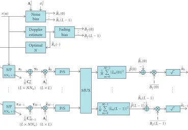
The estimatesBv(l) andBf(l) can be obtained by using the same procedure given in [23, 24]. Figure 3 shows the re-sulting multipath searcher. The Doppler estimate depicted
in Figure 3 is required during the determination of Rx(i)
and, hence,Nopt and the fading bias coefficientBf(l) [25].
Figure 4shows the SNR gain for different values of Doppler
frequencies. Moreover, Nopt for different values of Doppler frequencies has been shown inFigure 5.
4.2. Difficulties
The main problem facing the least-squares multipath search-er ofFigure 3is the ill-conditioning of the pulse-shaping ma-trixAL, which increases with the sampling resolution.Figure 6plots the condition number of the matrixAL(in dB) versus the oversampling factorNu.
180 160 140 120 100 80 60 40 20 0
SNR
gain
0 50 100 150 200 250
N
Maximum (Nopt)
fd=10
fd=20
fd=30
fd=40
fd=50
fd=80
Figure4: SNR gain versusNforK=256 andTc=8.138
microsec-onds and for different Doppler frequencies.
to extract and incorporate into the design of the adaptive solution a priori knowledge about the multipath channel.
5. AN ADAPTIVE PROJECTION TECHNIQUE
We now describe an adaptive projection technique for chan-nel estimation that exploits a priori information about the channel for enhanced accuracy. The technique replaces the least squares ofSection 4by an adaptive filter. The proposed method can be described as follows.
Recall that we need to solve least-squares problems of the form (32), that is,
zm=arg min
zm ym−ALzm 2
(51)
for successive values ofm, where
ym= 1
NC ∗
mrm. (52)
We will denote the entries of the successiveym by{dm(i)}. Clearly, the solution of (51) can also be approximately at-tained by training an adaptive filter that uses the{dm(i)}as reference data and the rows of theL×Lmatrix AL as re-gression data. We will denote the rows ofALby{ui}. Since AL has onlyL rows, the adaptive filter is cycled repeatedly through these regression rows until sufficient convergence is obtained. In addition, it is explained inAppendix Chow we can extract useful information about the channel such as its region of support (i.e., the region over which the channel taps are most likely to exist) and the largest amplitude that any of its peaks can achieve. This information can be exploited by the adaptive solution as explained below in order to enhance the accuracy and the resolution of the resulting multipath searcher. Thus the adaptive implementation can be described as follows.
(1) The received signal r(n) is applied to a bank of matched filtersC∗min order to generate the vectors{ym}.
600 500 400 300 200 100 0
Nop
t
20 40 60 80 100 120
fd(Doppler frequency)
OptimalNversus Doppler frequency
Figure5: OptimumNforK=256 andTc=8.138 microseconds.
120 100 80 60 40 20 0
Data
mat
rix
co
ndition
n
umber
(dB)
1 2 3 4 5 6 7 8
Nu
Figure6: Condition number ofALversusNu.
(2) A parallel-to-serial converter is applied to eachymin order to form the reference sequence{dm(i)}.
(3) An adaptive filter of weight vectorwimis used to es-timatezmat theith iteration (i.e.,wmi is the estimate ofzm at iterationi). The regression vectoruiis obtained from the rows ofAL. The adaptive filter is iterated repeatedly in a cyclic manner over the rows ofALuntil sufficient performance is attained.
r(n) (m+1)NNu−1
n=mNNu
r(n)ym(0) | · |2 M1 M−1
m=1 (·)
Jf(τ) Extract
channel information
Feed information in the projection
operationP · · ·
N
S/P
NNu×1
r0
1
NC∗0
y0
P/S d0(i) AL ui w0i P
− z0
. . .
S/P
NNu×1
rM−1 yM−1
1
NC∗M−1 AL ui wMi −1 P − P/S dM−1(i)
. . . .
. .
zM−1
Proceed as in the multipath searcher of
Figure 3
α0
αL−1
. . .
Figure7: An adaptive multipath resolving scheme using successive projections.
inhtranslate into zero taps in the estimates ofzm). Specifi-cally, the adaptive filter weight vectorwimis updated as fol-lows:
wmi =
⎧ ⎨ ⎩
wm
i−1+μ(i)u∗i
dm(i)−uiwmi−1
fori=Np, 2Np,. . .,
P#wmi−1+μ(i)u∗idm(i)−uiwmi−1$ fori=Np, 2Np,. . . . (53)
Hereμ(i) is a step-size parameter,P refers to the projection procedure, andNpis an integer greater than or equal to one and less than or equal to the total number of iterations per-formed.
(5) The successive projections are based on information obtained from the upper branch of the block diagram in
Figure 7. The first branch extracts information about the
channel region of support and maximum amplitude. This information is extracted by noncoherently averaging the out-put of the matched filter bank to formJf(τ). The adaptive filter weight vector is successively projected onto the set of possible elements satisfying the constraints (e.g., tap loca-tions and amplitudes should lie within the ranges specified by the a priori information). The adaptive filter weight vec-tor is iterated till it reaches steady state. For instance, when the upper branch finds 3 taps, it gives a rough estimation for the location and amplitude of these taps. The projection scheme within the adaptive filter blocks checks the number of nonzero taps inwi, and forces the taps that are out of the detected range by the upper branch to zero.
5.1. Simulation results
The robustness of the proposed algorithm in resolving over-lapping multipath components is tested by computer
simulations. In the simulations, a typical IS-95 signal is gen-erated, pulse shaped, and transmitted through various mul-tipath channels. The total power gain of the channel com-ponents is normalized to unity.Figure 8is a sample simula-tion that compares the output of the proposed adaptive algo-rithm to the output of the block least-squares multipath re-solving technique ofSection 4for a two-ray fading multipath channel. The first plot shows the considered two-ray channel in the simulation. The second and third plots, respectively, show the output of block least-squares and block regularized least-squares stages. It is clear that both least-squares tech-niques lead to significant errors in the estimation of the time and amplitude of arrival of the first arriving ray. The last plot shows the output of the proposed estimation scheme. It is clear that the proposed algorithm is more accurate than least-squares techniques. Here we may add that it was noted that the algorithm converges in around 30–50 runs. In this simu-lation, we have assumed 128 spreading sequences (K=128), each chip is upsampled by order of 8 (Nu=8), the upsam-pled receiving vector is partitioned into 8 subblocks (M=8), the receiving SNR before despreading is−15 dB and finally the adaptive filter step size is 0.7 (μ=0.7).
Figure 9shows the estimation time delay absolute error
0.8 0.6 0.4 0.2 0
A
m
plitude
0 5 10 15 20
Delay (Tc/8)
Channel
(a)
10 5 0 −5
A
m
plitude
0 5 10 15 20
Delay (Tc/8)
LS solution
(b)
1.5 1 0.5 0 −0.5 −1
A
m
plitude
0 5 10 15 20
Delay (Tc/8)
Regularized LS solution
(c)
0.8 0.6 0.4 0.2 0
A
m
plitude
0 5 10 15 20
Delay (Tc/8)
Proposed method
(d)
Figure8: Simulation results (K =128,Nu =8,M=8, andμ=
0.7).
is 0.7 (μ = 0.7). Please note that different fading frequen-cies change the effective again after despreading according to (47).
6. RECEPTION WITH AN ANTENNA ARRAY
Using an antenna array at the base station can improve the location estimation by providing both the TOA and AOA information. An antenna array receiver integrates multiuser detection and beamforming with rake reception in order to
0.35 0.3 0.25 0.2 0.15 0.1
Dela
y
M
AE
(
μ
s)
0 1 2 3 4 5 6 7 8 9 10
Estimated period (s)
fd=10 Hz
fd=40 Hz
fd=80 Hz
−10 −12 −14 −16 −18 −20 −22
A
m
plitude
relati
ve
M
SE
(dB)
0 1 2 3 4 5 6 7 8 9 10
Estimated period (s)
fd=10 Hz
fd=40 Hz
fd=80 Hz
Figure9: Simulation results for fading channels inFigure 8(K =
128,Nu=8,M=8, andμ=0.7).
mitigate multiuser interference, cochannel interference and fading.
Thus consider anNa-element antenna array at the base station. In this case, the channel model (1) is replaced by
h(n)=
L−1
l=0
αlxul(n)δ(n−l)a
θl
, (54)
whereh(n) is now anNa×1 vector,a(θl) is theNa×1 array response as a function of the AOA of thelth multipath and it is given by
aθl
=%1,ej2π(d/λ) sin(θl),. . .,ej2π((M−1)d/λ) sin(θl)&T. (55)
Here, θl is the AOA of the received signal over the lth multipath,dis the antenna spacing, andλis the wavelength corresponding to the carrier frequency. Likewise, the received signal in (3) is replaced by
r(n)=cu(n)p(n)h(n) +v(n), (56) wherer(n) is now anNa×1 vector. We can again use the arguments ofSection 3to replace (10) by
R=ACxAθH+V, (57) whereRis anLr×Nareceived matrix defined as
Rr1,r2,. . .,rNa
andrnis the received vector of lengthLrover thenth antenna array, that is,
rn=colrn(0),rn(1),. . .,rn
Lr−1
,
n=1, 2,. . .,Na.
(59)
Moreover,Vis the noise matrix
Vv1,v2,. . .,vNa
, (60)
wherevnis the noise vector at thenth antenna array,
vn=colv(0),v(1),. . .,vLr−1
,
n=1, 2,. . .,Na
(61)
andHis anLNa×NaToeplitz path gain matrix whose first column is determined by
h=colα0,α1,. . .,αL−1, 0, 0,. . ., 0
. (62)
FinallyAθ is anL×LNamatrix that contains the array re-sponses:
AθAθ,1,Aθ,2,. . .,Aθ,Na
, (63)
where
Aθ,n=
⎡ ⎢ ⎢ ⎢ ⎣
ej2π((n−1)d/λ) cos(θ0)
. ..
ej2π((n−1)d/λ) cos(θL−1) ⎤ ⎥ ⎥ ⎥ ⎦
n=1, 2,. . .,Na.
(64)
The problem we are interested in is that of estimating the
{αl}from the received matrixRin (58).
6.1. The partitioned adaptive receiver
As inSection 4, we partitionRinto smaller matrices,Rm, of sizeNNu×Naeach. The matrixRmwill then satisfy an equa-tion of the form
Rm=AmCm
xAθH+Vm (65)
with{Am,Cm
x}similar to{A,Cx}in (10) but of smaller di-mensions, and whereVmis defined by
Vm=vm,1,. . .,vm,Na
, vm,n=col
vnmNNu
,. . .,vn(m+ 1)NNu−1
,
n=1, 2,. . .,Na.
(66)
Then, in view of the earlier discussion, we can use the same algorithm that we used in the case of single antenna.
(1) Partition the received matrixRintoMsmallerNNu×
Na matricesRm with NNu samples on each column given by
rm,n=col
rnmNNu
,. . .,rn(m+ 1)NNu−1
. (67)
(2) Introduce theNNu×Lcorrelation (despreading) ma-trix and theL×Lfading matrixXmas defined in (29). (3) Multiply vec(Rm) from the left by (1/N)C∗θ,m, withm=
0, 1,. . .,M−1, whereCθ,mis theNNu×LNamatrix defined by
Cθ,m=Cm
Aθ,1,Aθ,2,. . .,Aθ,Na
. (68)
The correlated (despreaded) output is denoted by
ym= 1
NC ∗
θ,mvec
Rm. (69)
WhenN is large enough, and similar to (31),ymcan be approximated by
ym≈ALXmh+ 1
NC ∗
θ,mvec
Vm. (70)
The resulting signalymin (70) is similar to the signal in (31), albeit with higher SNR due to the use of the antenna array. Therefore, the proposed estimation al-gorithm (32)–(49) for the single antenna case can be used as well.
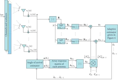
The system model for the resulting multiantenna adaptive re-ceiver is illustrated inFigure 10.
6.2. Estimating the array response
We still need to estimate the array response matrixAθ. For the received signalRin (57) of sizeLr×Na, we define a cor-relation matrix, as in (17), as follows:
Y= 1
KC ∗R= 1
KC
∗ACxAθH+ 1 KC
∗V, (71)
whereCwas defined in (16) andKis the length of the spread-ing sequence. Now replaceAθHbyZ, so that
Y= 1
KC ∗ACx
P
Z+ 1
KC ∗V,
Y=PZ+ 1
KC ∗V.
(72)
The least-square estimate ofZis given by
Z=P∗P−1P∗Y. (73)
Now, in order to estimateAθ fromZ, we need an estimate of the channel matrix H. It can be estimated from (74) by noting that the matrixAθ,1(the firstL×Lblock ofAθ) is an identity matrix, so that
y1= 1
KC
∗ACxAθh+ 1 KC
∗v 1
= 1
KC ∗ACxAθ
,1h+ 1
KC ∗v
1
= 1
KC ∗AC
xh+ 1
KC ∗v
1,
User
Channe
ls
and
scatt
er
ers
. .. . . .
. . .
. . .
. . . .
. . . ..
v1(n) r1(n)
v2(n) r2(n)
vNa(n) rNa(n)
[·] R
N
R
S/P
NNu×1 R0
vec (·)vec (R0) y0 .
. .
. . .
. . . S/P
NNu×1 RM−1
vec (·)vec (RM−1) ym−1
Adaptive estimator given in Figure 4
α0
. . .
αL−1
Angle of arrival estimator
a(θ1) . . . a(θL)
Array response matrix of each antenna
Aθ,1 . . . Aθ,Na
[·] Aθ 1
NC∗θ,0 · · · N1C∗θ,M−1
C0 CM−1 · · ·
α0. . .αL−1
Figure10: An adaptive multipath resolving scheme using an antenna array receiver.
wherehis defined in (62) andhis anL×1 vector that con-tains the firstLelements of h. Moreover,v1 andy1are the first column ofVandY, respectively. Soh can now be es-timated using (74) in the same manner ashwas estimated fromymin (30) by using (49). Usinghto createH, the least-squares estimate ofAθcan be obtained as
Aθ=ZH∗ HH∗−1. (75)
6.3. Simulation results with antenna array
The robustness of the proposed algorithm in resolving over-lapping multipath components when the base station has an array of antennas is tested by computer simulations. In the simulations, a typical IS-95 signal is generated, pulse shaped, and transmitted through various multipath chan-nels. The total power gain of the channel components is nor-malized to unity. We have considered 4 antennas at the base station andFigure 11compares the simulation results when there are multiple antennas and single antenna at the base station. In this simulation, we have assumed 128 spreading sequences (K =128), each chip is upsampled by order of 8 (Nu=8), the upsampled receiving vector is partitioned into 8 subblocks (M = 8) and the adaptive filter step size is 0.7 (μ=0.7).
7. CONCLUSIONS
This paper develops two overlapping multipath resolving methods (adaptive and nonadaptive), and illustrates how the adaptive solution can be made robust to fast channel fad-ing and data ill-conditionfad-ing by extractfad-ing and exploitfad-ing a
priori information about the channel. The proposed tech-niques are further extended to the case with antenna arrays at the base station. Simulation results illustrate the perfor-mance of the techniques.
APPENDICES
A. PROOF OF(19)
To simplify (1/K)C∗ACx, we start with the givenAin (6) and express it as
ATop(p),
pcolp(0),p(1),. . .,p(P−1), (A.1) where the notation Top(p) denotes the lower-triangular Toeplitz matrix determined byp. Let
ciith column ofC, cx,iith column ofCx,
(A.2)
then
C∗ACx=
⎡ ⎢ ⎢ ⎢ ⎢ ⎢ ⎢ ⎢ ⎢ ⎣
c∗1
.. .
c∗K
⎤ ⎥ ⎥ ⎥ ⎥ ⎥ ⎥ ⎥ ⎥ ⎦
Top(p)cx,1 | · · · | cx,L−1
. (A.3)
Now note that for anym×1 vector vandn×mToeplitz matrix Top(w), wherewisl×1 thatl < n, we have
×10−7 4.5
4 3.5 3 2.5 2 1.5 1 0.5 0 Dela y M AE (s)
0 1 2 3 4 5 6 7 8 9 10
Estimation period (s)
Multiple-antenna receiver (N=4) with single-antenna receiver
fd=10, multiple antenna
fd=40, multiple antenna
fd=80, multiple antenna
fd=10, single antenna
fd=40, single antenna
fd=80, single antenna
(a) 2 0 −2 −4 −6 −8 −10 −12 −14 −16 A mplitude relati ve M SE (dB)
0 1 2 3 4 5 6 7 8 9 10
Estimation period (s)
Multiple-antenna receiver (N=4) with single-antenna receiver
fd=10, multiple antenna
fd=40, multiple antenna
fd=80, multiple antenna
fd=10, single antenna
fd=40, single antenna
fd=80, single antenna
(b)
Figure11: Simulation results for the given channel inFigure 8(K=128,Nu=8,M=8 andμ=0.7).
where Top(v) isn×lToeplitz. Then (A.3) can be written as
C∗ACx=
⎡ ⎢ ⎢ ⎢ ⎢ ⎢ ⎢ ⎢ ⎢ ⎣
c∗1
.. .
c∗K
⎤ ⎥ ⎥ ⎥ ⎥ ⎥ ⎥ ⎥ ⎥ ⎦
Topcx,1
| · · · | Topcx,L−1
p.
(A.5) Due to the orthogonality property of the spreading sequences we have
Rc(τ)=
K−1
j=0
c∗(j)c(j+τ)=
⎧ ⎨ ⎩K
, τ=0,
ρ≈0, τ=0 (A.6) so that
c∗i ·cx,l≈
⎧ ⎪ ⎪ ⎪ ⎨ ⎪ ⎪ ⎪ ⎩ K
K−1
j=0
xl(j), i=l,
0, i=l
(A.7) and, therefore, ⎡ ⎢ ⎢ ⎢ ⎢ ⎢ ⎢ ⎢ ⎢ ⎣
c∗1
.. .
c∗K
⎤ ⎥ ⎥ ⎥ ⎥ ⎥ ⎥ ⎥ ⎥ ⎦
Topcx,l
=Top ⎛ ⎜ ⎜ ⎜ ⎜ ⎜ ⎜ ⎜ ⎜ ⎜ ⎜ ⎜ ⎜ ⎜ ⎜ ⎜ ⎜ ⎜ ⎜ ⎝ ⎡ ⎢ ⎢ ⎢ ⎢ ⎢ ⎢ ⎢ ⎢ ⎢ ⎢ ⎢ ⎢ ⎣ 0 .. . K
K−1
j=0
xl(j)
0 .. . ⎤ ⎥ ⎥ ⎥ ⎥ ⎥ ⎥ ⎥ ⎥ ⎥ ⎥ ⎥ ⎥ ⎦
only thelth row is nonzero
⎞ ⎟ ⎟ ⎟ ⎟ ⎟ ⎟ ⎟ ⎟ ⎟ ⎟ ⎟ ⎟ ⎟ ⎟ ⎟ ⎟ ⎟ ⎟ ⎠ . (A.8)
Substituting (A.8) into (A.5) gives
C∗ACx=KTop(p) diag
K−1
j=0
x0(j),. . ., K−1
j=0
xL−1(j)
=KALXK,
(A.9)
where
ALTop(p),
XK diag
K−1
j=0
x0(j),. . ., K−1
j=0
xL−1(j)
. (A.10)
B. NOISE PROPERTY
From (41), we have
v(0)=c(mN)v(0) +c(mN+ 1)v(1) +· · ·+c(m+ 1)N−1v(N−1),
v(1)=c(mN)v(1) +c(mN+ 1)v(2) +· · ·+c(m+ 1)N−1v(N) ..
..
(B.1)
Then, wheni= j,
Ev(i)v∗(j)
=E ⎛ ⎝N−1
p=0 N−1
q=0
c(mN+p)v(p+i)c(mN+q)v(q+j)∗
=E ⎛ ⎜ ⎜ ⎜ ⎝
N−1
p=0 N−1
q=0 p+i=q+j
c(mN+p)v(p+i)c(mN+q)v(q+j)∗
⎞ ⎟ ⎟ ⎟ ⎠
+E ⎛ ⎜ ⎜ ⎜ ⎜ ⎝
N−1
p=0 N−1
q=0 p+i=q+j
c(mN+p)v(p+i)c(mN+q)v(q+j)∗
⎞ ⎟ ⎟ ⎟ ⎟ ⎠
=σ2 v
N−1
p=0 N−1
q=0 p+i=q+j
c(mN+p)c(mN+q)∗
N−1
p=0c(mN+p)c∗(mN+p+i−j)≈0
+ N−1
p=0 N−1
q=0 p+i=q+j
c(mN+p)c(mN+q)∗Ev(p+i)v(q+j)∗
=0
≈0.
(B.2)
It follows thatv(i) andv(j) are uncorrelated fori=j.
C. EXTRACTING A PRIORI CHANNEL INFORMATION
In this appendix we explain how to extract useful a priori channel information from the received signal [26]. This in-formation is used inSection 5by the adaptive searcher for resolving overlapping multipath components.
(1) A power delay profile (PDP) is evaluated as follows:
Jf(τ) 1
M
M−1
m=0
N1
(m+1)NNu−1
n=mNNu
r(n)ym(n) 2
. (C.1)
(2) Theregion of supportof the power delay profile, sayRf, is determined by comparing the PDP with a thresh-old λf. The region of support refers to the region of the delay (τ) that might contain significant multipath components:
τ∈Rf ifJf(τ)> λf. (C.2)
We restrictRf to the first continuous region of delays. In other words,Rf starts from the earliest delay that is higher than the threshold until the value ofτat which the PDP falls below the threshold.
(3) The peak of the PDP is determined along with the de-lay that corresponds to the peak. Letτf denote the de-lay of the peak ofJf(τ):
τf arg max
τ Jf(τ), τ∈Rf. (C.3) Moreover, letmf denote the value of the peak ofJf(τ):
mf max
τ Jf(τ), τ ∈Rf. (C.4)
(4) The number of fading overlapping multipath compo-nents that exist in the region of support,Rf, is deter-mined by using the multipath detection algorithm of [26]. Let the number of overlapping multipath com-ponents be denoted byO.
In summary, the following a priori information can be used in the multipath resolving stage.
(1) The delay of the ray to be resolved is confined toRf. (2) The number of fading overlapping multipath
compo-nents that exist inRf is equal toO.
(3) The maximum amplitude of any ray in this region is less than or equal to the square root of the maximum value ofJf(τ) after equalizing for the noise and fad-ing biases that may arise in this value. This value is equal to(Cf(mf −Bv), whereBvandCf are two noise and fading biases that can be calculated as described in (49)-(50).
ACKNOWLEDGMENTS
This material was based on work supported in part by the National Science Foundation under Awards CCR–0208573 and ECS-0401188. Preliminary versions of some results in this work appeared in the conference publications [24,27].
REFERENCES
[1] FCC Docket no. 94-102, “Revision of the commission’s rules to ensure compatibility with enhanced 911 emergency calling,” Tech. Rep. RM-8143, July 1996.
[2] J. J. Caffery and G. L. Stuber, “Overview of radiolocation in CDMA cellular systems,”IEEE Communications Magazine, vol. 36, no. 4, pp. 38–45, 1998.
[3] J. O’Connor, B. Alexander, and E. Schorman, “CDMA infrastructure-based location finding for E911,” inProceedings of 49th IEEE Vehicular Technology Conference (VTC ’99), vol. 3, pp. 1973–1978, Houston, Tex, USA, May 1999.
[4] S. Fischer, H. Koorapaty, E. Larsson, and A. Kangas, “Sys-tem performance evaluation of mobile positioning methods,” inProceedings of 49th IEEE Vehicular Technology Conference (VTC ’99), vol. 3, pp. 1962–1966, Houston, Tex, USA, May 1999.
[5] S. Tekinay, E. Chao, and R. Richton, “Performance bench-marking for wireless location systems,”IEEE Communications Magazine, vol. 36, no. 4, pp. 72–76, 1998.
[6] J. J. Caffery and G. L. Stuber, “Radio location in urban CDMA microcells,” inProceedings of 6th IEEE International Sympo-sium on Personal, Indoor and Mobile Radio Communications (PIMRC ’95), vol. 2, pp. 858–862, Toronto, Ontario, Canada, September 1995.
[7] A. Ghosh and R. Love, “Mobile station location in a DS-CDMA system,” inProceedings 48th IEEE Vehicular Technology Conference (VTC ’98), vol. 1, pp. 254–258, Ottawa, Ontario, Canada, May 1998.
[8] C. Drane, M. Macnaughtan, and C. Scott, “Positioning GSM telephones,”IEEE Communications Magazine, vol. 36, no. 4, pp. 46–54, 1998.
UMTS Terminals and Software Radio, pp. 10/1–10/6, Glasgow, UK, April 1999.
[10] S. Sakagami, S. Aoyama, K. Kuboi, S. Shirota, and A. Akeyama, “Vehicle position estimates by multibeam antennas in multi-path environments,”IEEE Transactions on Vehicular Technol-ogy, vol. 41, no. 1, pp. 63–68, 1992.
[11] J. M. Zagami, S. A. Parl, J. J. Bussgang, and K. D. Melillo, “Pro-viding universal location services using a wireless E911 loca-tion network,”IEEE Communications Magazine, vol. 36, no. 4, pp. 66–71, 1998.
[12] T. S. Rappaport, J. H. Reed, and B. D. Woerner, “Position lo-cation using wireless communilo-cations on highways of the fu-ture,”IEEE Communications Magazine, vol. 34, no. 10, pp. 33– 41, 1996.
[13] L. A. Stilp, “Carrier and end-user applications for wireless lo-cation systems,” inWireless Technologies and Services for Cellu-lar and Personal Communication Services, vol. 2602 of Proceed-ings of the SPIE, pp. 119–126, Philadelphia, Pa, USA, October 1995.
[14] I. J. Paton, E. W. Crompton, J. G. Gardiner, and J. M. Noras, “Terminal self-location in mobile radio systems,” in Proceed-ings of 6th International Conference on Mobile Radio and Per-sonal Communications, vol. 1, pp. 203–207, Coventry, UK, De-cember 1991.
[15] A. Giordano, M. Chan, and H. Habal, “A novel location-based service and architecture,” inProceedings of 6th IEEE Interna-tional Symposium on Personal, Indoor and Mobile Radio Com-munications (PIMRC ’95), vol. 2, pp. 853–857, Toronto, On-tario, Canada, September 1995.
[16] N. R. Yousef, A. H. Sayed, and N. Khajehnouri, “Detection of fading overlapping multipath components,” to appear in Sig-nal Processing.
[17] A. H. Sayed, A. Tarighat, and N. Khajehnouri, “Network-based wireless location: challenges faced in developing techniques for accurate wireless location information,”IEEE Signal Pro-cessing Magazine, vol. 22, no. 4, pp. 24–40, 2005.
[18] J. J. Caffery and G. L. Stuber, “Vehicle location and tracking for IVHS in CDMA microcells,” in Proceedings of 5th IEEE International Symposium on Personal, Indoor and Mobile Ra-dio Communications (PIMRC ’94), vol. 4, pp. 1227–1231, The Hague, The Netherlands, September 1994.
[19] Z. Kostic, I. M. Sezan, and E. L. Titlebaum, “Estimation of the parameters of a multipath channel using set-theoretic de-convolution,”IEEE Transactions on Communications, vol. 40, no. 6, pp. 1006–1011, 1992.
[20] T. G. Manickam and R. J. Vaccaro, “A non-iterative deconvo-lution method for estimating multipath channel responses,” inProceedings of IEEE International Conference on Acoustics, Speech, and Signal Processing (ICASSP ’93), vol. 1, pp. 333–336, Minneapolis, Minn, USA, April 1993.
[21] T. S. Rappaport,Wireless Communications: Principles & Prac-tice, Prentice-Hall, Upper Saddle River, NJ, USA, 1996. [22] S. Glisic and B. Vucetic,Spread Spectrum CDMA Systems for
Wireless Communications, Artech House, Boston, Mass, USA, 1997.
[23] N. R. Yousef and A. H. Sayed, “A new adaptive estimation al-gorithm for wireless location finding systems,” inProceedings of 33rd Asilomar Conference on Signals, Systems, and Comput-ers (ACSSC ’99), vol. 1, pp. 491–495, Pacific Grove, Calif, USA, October 1999.
[24] N. R. Yousef and A. H. Sayed, “Adaptive multipath resolving for wireless location systems,” inProceedings of 35th Asilomar Conference on Signals, Systems and Computers (ACSSC ’01), vol. 2, pp. 1507–1511, Pacific Grove, Calif, USA, November 2001.
[25] A. Jakobsson, A. L. Swindlehurst, and P. Stoica, “Subspace-based estimation of time delays and Doppler shifts,” IEEE Transactions on Signal Processing, vol. 46, no. 9, pp. 2472–2483, 1998.
[26] N. R. Yousef and A. H. Sayed, “Detection of fading overlap-ping multipath components for mobile-positioning systems,” inProceedings of IEEE International Conference on Communi-cations (ICC ’01), vol. 10, pp. 3102–3106, Helsinki, Finland, June 2001.
[27] N. R. Yousef and A. H. Sayed, “Robust multipath resolving in fading conditions for mobile-positioning systems,” in Pro-ceedings of 17th National Radio Science Conference (NRSC ’00), vol. 1, no. C19, pp. 1–8, Minufiya, Egypt, February 2000.
Nabil R. Yousefreceived the B.S. and M.S. degrees in electrical en-gineering from Ain-Shams University, Cairo, Egypt, in 1994 and 1997, respectively, and the Ph.D. degree in electrical engineering from the University of California, Los Angeles, in 2001. He was a StaffScientist at the Broadband Systems Group (2001–2005), Broadcom Corporation, Irvine, Calif. His work at Broadcom in-volved developing highly integrated systems for cable modems, ca-ble modem termination systems, wireless broadband receivers, and DTV receivers. He is currently the Director of Systems Engineering at Newport Media Inc., Lake Forest, Calif. He is involved in devel-oping highly integrated receivers for mobile TV standards such as DVB-H, T-DMB, ISDB-T and MedisFlo. His research interests in-clude adaptive filtering, equalization, OFDM and CDMA systems, wireless communications, and wireless positioning. He has over 30 issued and pending US patents. He is the recipient of a 1999 Best Student Paper Award at an international meeting for work on adap-tive filtering, and of the 1999 NOKIA Fellowship Award. He re-ceived many awards for his innovations from Motorola, Broadcom, and Newport Media Inc.
Ali H. Sayedis Professor and Chairman of electrical engineering at the University of California, Los Angeles. He is also the Prin-cipal Investigator of the UCLA Adaptive Systems Laboratory (www.ee.ucla.edu/asl). He has over 250 journal and conference publications, he is the author of the text-book Fundamentals of Adaptive Filtering
(Wiley, New York, 2003), and is coau-thor of the research monograph
Indefi-nite Quadratic Estimation and Control(SIAM, Philadelphia, PA, 1999) and of the graduate-level textbook Linear Estimation
He received the 1996 IEEE Donald G. Fink Award, 2002 Best Paper Award from the IEEE Signal Processing Society, 2003 Kuwait Prize in Basic Science, 2005 Frederick E. Terman Award, and is coauthor of two Best Student Paper Awards at international meetings (1999, 2001). He is a Member of the editorial board of the IEEE Signal Pro-cessing Magazine. He has also served twice as Associate Editor of the IEEE Transactions on Signal Processing, and as Editor-in-Chief of the same journal during 2003–2005. He is serving as Editor-in-Chief of the EURASIP Journal on Applied Signal Processing and as General Chairman of ICASSP 2008.
Nima Khajehnouri received the B.Sc. de-gree in electrical engineering from Sharif University of Technology, Tehran, Iran, in 2001, and the M.S. degree in electrical en-gineering from the University of California, Los Angeles (UCLA) in 2002 with empha-sis on signal processing. Since 2003, he has been pursuing the Ph.D. degree in electrical engineering at UCLA. His research focuses on signal processing techniques for