A computationally efficient approximation algorithm for analyzing open queueing networks with blocking

A Cornput.ationally Efficient Appr-oximat.ion

Algorithm for Analyzing

Open Queueing Networks with Blocking

by

H.G. Perras

P.M.

Snyder

Center for Communications and Signal Processing Cornp uter Science Depar-tment

North Carolina State University

Sept.ernber 1986

Abstract

A computationally efficient algorithm for analyzing approximately open queue-ing networks with blockqueue-ing is presented. This algorithm is based on an earlier pro-cedure proposed by Altiok and Perros [3"]. However, unlike this earlier propro-cedure, the proposed new algorithm has minimal time and space requirements. It permits, therefore, the analysis of large and complicated networks. It also makes implemen-tation easy, and software development feasible. Numerical experience with this algorithm shows that the approximate results seem to have an acceptable error level.

Kev words: queueing networks, finite queues, blocking, decomposition

Introduction

Queueing networks with finite queue capacities are useful in modelling com-puter systems, distributed systems, telecommunication systems and also

manufac-turing systems. A queueing network with finite queue capacities can be thought of

as a set of arbitrarily linked finite queues. Blocking arises due to limitations imposed on queue capacities. The flow of units through one queue may be blocked when the capacity limitation of another quell.e is reached. Several types of blocking

mechanisms have been considered in the literature so far. These blocking

mechan-isms arose out of various studies of real-life systems.

Onvural and Perras [16] have classified the most commonly used blocking

methods as follows:

Type 1: A customer upon completion of its service at queue i choses to enter desti-nation queue j. If at that moment queue j is full, then the customer is forced to wait in front of server i until it enters destination queue j.

Type 2: A customer in queue i declares its destination queue (queue j) before it starts its service. If queue j is full, then its server becomes blocked and it cannot serve the customer. When a departure occurs from destination queue

i.

then its server becomes unblocked and the customer begins its service.

Under this blocking type one can distinguish two sub-categories depending upon whether the customer is allowed to occupy the position in front of the blocked

Type 3: A customer upon service completion at queue i attempts to join destination qlleue j. If queue j is ittll, then the customer receives another service at queue i. This is repeated until the customer completes a service at queue i at a moment that

the destination node is not full.

Within this category, we distinguish two types:

Type 3.1: Once the customer's destination is determined it cannot be altered.

Type 3.2: A new destination node is chosen at each service completion independent of the destination previously chosen.

A comparison between these blocking mechanisms can be found in Onvural and Perras [16].

Queueing networks with blocking are in general difficult to treat. In particular, closed-form solutions for steady-state distributions are not generally attainable. Therefore, approximations, numerical techniques and simulation are used for the analysis of such queueing networks. Certain queueing networks with blocking, however, have been reported as having a product-form solution. These networks operate under a 3.2 type of blocking, and require assumptions so that they can satisfy reversibility. (For results see Kelly [12], Hordijk and Van Dijk [II], Yao and Buzacott [24], and Le Ny [15].)

Approximate studies of some particular configurations of open queueing net-works wit.. blocking have also been reported in the literature. A well-known confi-guration is the tandem conficonfi-guration consisting of finite queues in series. Approxi-mate studies of such configurations have been reported by Hillier and Boling [10], Caseau and Pujolle [7], Altiok [1], Perros and Altiok [18], Gershwin [8], Suri and Diehl [21], Bocharov and Rokhas [4], Brandwajn and [ow [6], Kelly [13], Pollock and Birge [20], and Goto, Takahashi and Hasegawa [9]. Other configurations that have been considered in the literature are split and merge configurations. Approximate studies of such configurations have been reported by Perros [17] and Altiok and Perros [2].

con-figurations. Labetoulle and Pujolle [14] analyzed arbitrary configurations of open networks with blocking under blocking mechanism type 3.1. They employed an algorithm similar to the one reported in Caseau and Pujolle [7]. Further validation of this algorithm is needed. Yao and Buzacott [24] reported on an approximation algorithm for analyzing closed queueing networks under blocking mechanism type 3.2 assuming Coxian service times and reversible routing. The algorithm gives the marginal queue-length probability distributions.

In this paper, we present a computationally efficient approximation algorithm for analyzing arbitrary configurations of open exponential queueing networks under type 1 blocking mechanism. This algorithm is based on an earlier algorithm pro-posed by Altiok and Perros [3]. Unlike the Altiok and Perros algorithm, however, the proposed algorithm has minimal time and space requirements. It permits, there-fore, the analysis of large and complicated networks, The class of queueing net-works to which this algorithm is applicable is described in the next section.

2. Arbitrary Configuration of Open Queueing Networks with Blocking

one queue. For simplicity, we have assumed in this paper that they all occur to one

particular queue (cf. Altiok and Perros [2]).

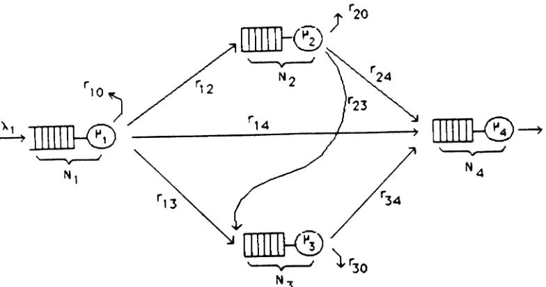
Figure 1: the three node configuration

Certain restrictions apply as to how' arbitrary' a configuration under study may be. In particular, a finite queue may not accept both external arrivals and input from other (upstream) queues. This restriction is necessary due to the fact that the

blocking mechanism considered in this paper is not consistent with the external arrival process, whereby a customer is lost (as opposed to being blocked) if it arrives

at a time that the queue is full. The topology of the queueing networks considered

then this graph may not contain directed cycles. This restriction is necessitated by the fact that the approximation algorithm does not take into account the problem of deadlock.

Blocking occurs due to the finite capacity of the queues. Type 1 blocking mechanism is assumed. In particular, a customer upon service completion at queue i attempts to join destination queue j. Blocking will occur ifat that instance queue j

is full. The blocking customer is forced to wait at queue i until it enters queue j. During this time the ith server is blocked and it cannot serve

any

other customers that might be waiting in its queue. Now, let us assume that there are k queues directly linked to queue j. Then, it is likely that at any instance there might be more than one blocking customer (each associated with one of these k queues). Obvi-ously, the total number of blocking customers at any instance may not exceed k. All blocking customers may be thought of as forming an imaginary blocking queue (although in effect they are waiting in front of their respective servers). When a customer at one of the k queues gets blocked by queue j it is placed at the end of the blocking queue. When a departure occurs from queue j, the unit at the top of the blocking queue is allowed to enter queue j. At that moment its associated server becomes unblocked. Thus, blocking customers are allowed to join queue j on a "first blocked-first-enter" basis.

each individual solution obtained is assumed to approximate the solution of that queue when it is part of the '-iueueing network. The parameters of each queue are revised as follows:

a) The arrival process at each queue is approximated by a Poisson distribution.

b) The original service mechanism of any queue that may become blocked is replaced by a process which uses Coxian-2 distributions to represent the delay a unit experiences at the queue because of blocking.

c) The capacity of each finite queue is augmented by as many positions as the number of upstream queues directly linked to it, i.e., queues from which it can receive units to be serviced. The capacity revision is necessary because the blocking mechanism considered in this paper allows a blocked server to act as an additional storage space for the blocking queue. This capacity revision does not apply to queues to which only external arrivals occurs.

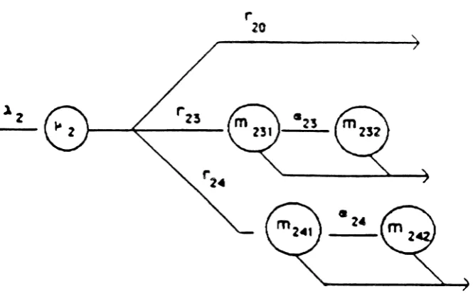
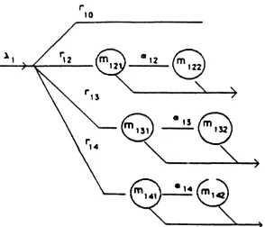
Figure 2: The four node configuration

The time that a blocked unit at queue 2 must wait in order to enter queue 3 depends not only on whether there is a unit from queue 1 waiting to enter queue 3, but also on the blocking experienced by units processed at queue 3 which require service at queue 4. Altiok and Perras [3] construct for each queue a very complicated phase-type structure which represents all possible blocking delays a unit may experience after it completes its service at this queue. This method has two shortcomings : first, a great deal of experience is required for the accurate construe-tion of the phase-type structure; second, the size of these structures gives rise to CPU complexity problems. As a result, it was only possible to analyze queueing networks of up to four queues.

representing all blocking delays a unit may experience upon service completion at a queue has a very simple structure. It can be written down very quickly a.id it is concise and consistent from queue to queue, thus making implementation easy and software development feasible. Also, the solution of each individual queue can be obtained very efficiently, seeing that the size of the matrix: which must be inverted is limited to one plus two times the number of possible destination queues.

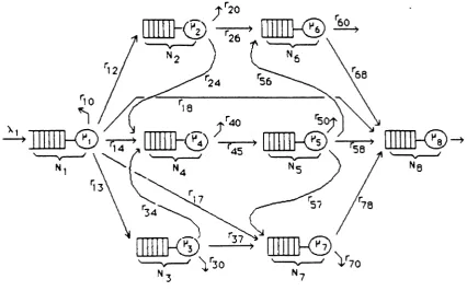
Figure 3: The eight node network

The approximation algorithm has been implemented for three, four and eight

this algorithm.

3. The approximation algorithm applied to the four node network

Consider a queueing network with blocking consisting of four single server queues linked as shown in figure 2. Customers arrive at the first queue only, according to a Poisson process with rate At. Service times are exponentially distri-buted with parameter ~i at queue i. Let N, denote the capacity ( including the one in service) of the ith node. N_2, N_3, N₄are assumed to be finite and N, is allowed to be finite or infinite.

Customers enter the network by joining the first queue. If N_l is assumed to be finite, units arriving when the buffer at queue 1 is full are lost. Upon service com-pletion at queue 1, a unit is sent to queue 2, 3, 4 with probability f12,f13,f14 respec-tively or the unit may depart from the network with probability flO . When a unit completes service at queue 2, it may be sent to queue 3 or queue 4, or it may leave the network, with probability r23,r24,rZO respectively. Frem queue 3, units proceed to queue 4 with probability r34 or depart from the network with probability r30 . All units completing service at queue 4 depart from the network with probability 1.

Blocking occurs in this network due to the finite capacity of queues 2, 3, and 4. Queue 4 may block qlleues I, 2 and 3; queue 3 may block quelles 1and 2 and queue 2 may block queue 1. Moreover, a unit being sent from quetle 3 to qtleUe 4 may find

enter at queue 3. Blocking is resolved on a " first-blocked-first-enter " basis.

Let Pi(n) be the probability that there are n units ( including the one in service) at queue i under equilibrium conditions and let 7rij(n) be the conditional probability that upon service completion at server i, there are n units at server j (including the one in service ).

3.1 The approximation algorithm for the case N₁=00

We first describe the algorithm assuming that the first queue, to which all external arrivals occur, has an infinite capacity. The modifications necessary when the first queue has a finite capacity are described in section 3.2.

The algorithm begins with the analysis of queue 4. Because of the network topology, queue 4 cannot become blocked. Since queues 1, 2 and 3 may send units to queue 4, the capacity of queue 4 is increased by 3 units and queue 4 is considered to be an MlM!1/N₄

+

3 queue. The equilibrium queue length distribution can be obtained from the classical MlM/l/N formulae once the overall arrival rate A4' is known. If queues 1, 2, and 3 are stable and never blocked, the input stream to queue 4 is Poisson with parameter ~4

=

1\1(r14

+

r12r24

+

r12r23r34+r13r34)· The relation-ship between

"4

and '\4' the rate at which units actually enter queue 4, is given by

the fixed-point expression

Once the equilibrium probability distribution of queue 4 is obtained, the

block-ing delay experienced by units at queues 1, 2, and 3 because queue 4 is at capacity

is represented by a Coxian-2 distribution. This distribution is constructed using the

phase-type structure developed by Altiok and Perros [3] and illustrated in figure 4.

This phase-type structure ret1ects all the possible delays a unit at queue i, i= 1,2,3,

may undergo, if at the moment it completes its service, its destination node, queue 4, is full. In particular a

. - - - \ '" 4 J I - - - o I l...

Figure 4: A phase-type representation of the blocking delay at queue 4.

unit entering this phase-type structure has already received service at queue i,

i= 1,2,3 and has selected queue 4 as its destination. With probability

event corresponds to the upper path in figure 4 . The other paths in figure 4 represent the event that ..l unit from queue i. i=1, 2, 3 , whose destination is queue 4 finds the buffer full. If no other units are already waiting for a buffer space, the

unit from queue i will be forced to wait at qlleue i until a service completion occurs

at queue 4. This time has an exponential distribution with parameter JL4. The path

in figure 4 corresponding to this event is the second one. If a unit arriving from queue i finds n units already awaiting a buffer space, the arriving unit will be blocked at queue i for n + 1 consecutive time periods, each exponentially

distri-buted with parameter J..L4. This situation corresponds to the two bottom branches in figure 4.

We determine the 1l"i4(.) using Little's relation. Let 1T4(n) be the conditional

pro-bability that a customer arriving at queue 4 sees n customers in the queue. Then

~41T4(N4)/~4=P4(N4+1) ~<!1T-t(N_ef

+

1)/J..L4

=

P4(N4

+

2)

~47T4(N₄

+

2)/~4= P4(N4

+

3) ·

Since we have obtained the equilibrium queue length distribution at queue 4, all

quantities are known except for the 11"4(.). Next, we estimate the 11"i4(·) using

h distribution illustrated in figure 4 are known, we can construct a

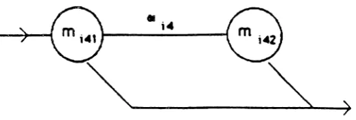
Coxian-2 representation of this phase-type distribution by determining its first three moments aid then fitting a Coxian-2 distribution, with parameters ffii41, mi42, (li4 to them. This Coxian-2 distribution, shown in figure 5, reflects the blocking delay at

queue 4.

·i~

)

Figure 5: Coxian-2 representation of the blocking delay at queue 4.

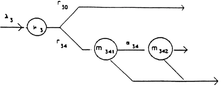
The third queue is now considered in isolation. The capacity of queue 3 is increased by two units since both queue 1 and queue 2 may be blocked by queue 3. The arrival process at queue 3 is assumed to be Poisson with parameter A31 where .\3

is determined from the fixed point problem

r 34

Figure 6: Service mechanism at queue 3

)

A three phase server of this type has a transition rate matrix with departure rate blocks having rank 1. This property allows the equilibrium queue length distribution to be written immediately in terms of the queue parameters, i.e.,

P3 (1)T

=

A3P3(O)[ 1 0 0 ]R

P3 (n)T=A3P3 (n-l)TR with

0 -1

J..L3 - r34J..L3

R=

-A3 _"'3+m~l - Ci34ffi341

-A3 0 "'3+ ffi342

and P3(n)=P3 (n)Te) where e3 is a column vector of all ones.

In the analysis of quelle 3, our method requires the construction of two Coxian-2 representations. This is done so that the solution of each node in isolation is both simple and consistent from node to node. First, the representation of the

augmented service mechanism at queue 3, which is shown in figure 6, is condensed

to a two phase Cox ian distribution with parameters m31,ffi32,(l). This Coxian-2 distri-bution incorporates the service delay at queue 3 and also delays due to blocking by

queue 4. This distribution is then used to construct a repr~sentation of the delay

experienced by units at queues 1 and 2 because queue 3 is at capacity. This

block-ing delay is represented in the form of a phase-type distribution shown below. It is constructed in a manner analogous to the one shown in figure 4.

1c \l ,s(Ns) - • ,5(NS . , )

r

'5

)

"'

&

_-_5_

m₁₂

Figure 7: The phase-type representation of the blocking delay at queue 3.

The conditional throughputs, 1T'){.), are obtained in the same way as in the case of queue 4. In particular, using Little's relation, we have

~37r3(N3)/~1= P~(~ ~+1)

~37T3(NJ+ 1)/J.L~= P3(:'\1+2)

1T23(N3)= r12 r2J1T3(N_{3)/ r}

1T13(N3+1)=r131T3(N3+ l)/r 'IT_{23(N 3}

+

1)

=

r12r231T3(N3

+

l)/r

with r= r12rn

+

rn The first three moments of the phase-type structure shown in

fig-ure 7 are then used to fit a Coxian - 2 distribution, with parameters ffii311 mi32' Cli3, to this phase-type distribution.

The arrival process at queue 2 is assumed to be Poisson with parameter ~2 where A.2 is calculated from the fixed point problem

with P2(N₂+ 1) a function of A2 and ~2=filAl. Figure 8 represents the augmented service mechanism at queue 2. It consists of the regular service given at queue 2

plus two Coxian-2 delays with parameters ffi231I m2321 CtD and ffi241, ffi242I Cl24

r 20

Figure 8: Service mechanism at queue 20

Queue 2 can be analyzed in isolation as an MIPH/l/N₂+1 queue. Its equilibrium

pro-bability distribution is given by

P2

(l)T="2p2 (0)[ 1 0 0 0 0 ]R P2 (n)T=A2P2 (n-l)TR with

fl.~ - f.L2r23 0 - J..L2f24 0 -1

-A2 A~+ffi231 - u23ffi231 0 0

R=

-A! 0 _"2+m232 0 0

-/\..., 0 0 _{A2+m2~1 - a~-+rn241}

-A,_- 0 0 0 _{"2+ ffi242}

anti P2(n)

=

P2

(n) Ie 2' where e2 is a column vector of all ones.

--Once tile equilibrium queue length distribution has been calculated we may

compute the conditional probability 1T12(N:!) using Little's relation in the same

manner as in quetle 2. The blocking delay experienced by units at queue 1 because queue 2 is at capacity is shown in figure 9. Using the first three moments of this

phase-type structure, we fit a Coxian-2 distribution with parameters ffi1211 ml221 (112·

1- ft12 (N2 )

r

20

Figure 9: A phase-type representation of the blocking delay at queue 2

Queue 1 can then be analyzed in isolation as an MlPH/l queue with the service

r

10

Figure 10: Service mechanism at queue 1 )

This service mechanism consists of the regular service plus 3 Coxian-2 distributions. Each of these Coxian-2 distributions reflects a blocking delay at a destination node. The equilibrium queue length distribution at queue 1 is then given by

Pl (l)T=~lPl (0)[ 10 0 0 0 0 O]R

PI (n)T==~lPl (n-l)TR

J..Ll - J..Ll r12 0 - f..L1r13 0 - f.11 rI 4 0

-AI _Al+m121 - cx12ffi₁₂₁ 0 _{0 0 0}

-AI 0 _{Al+m122 0 0 0 0}

R=

-AI 0 0 _{Al+m 131 - Cl13}ffi131 _{0 0}

- Al 0 0 0 _Al+m132 0 0

-AI 0 0 0 0 _{Al + ffi141 - Cl14}ffi₁₄₁

-AI 0 0 0 0 0 _Al+mI42

where PI (n)

=

PI (n)Tel and eI is a column vector of all ones. We note the

simi-larity in figures 6, 8, and 10 which greatly increases the ease of implementation for this algorithm.

3.2 The approximation algorithm for the case N_I<00

Now suppose that the capacity of the first queue is finite. In this case, the rate

~I at which units actually enter the first queue is not known. This means we do not

have available the ~i which we require in order to analyze the other queues in the network. This problem is circumvented by imbedding the approximation algorithm described above into an iterative scheme in which the value of ~1 is successively approximated. In particular, we select a starting value for ~l I call it ~lO, and make

one pass through the network, applying our algorithm. After computing the equili-brium queue length distribution at queue 1 we calculate ~ll

=

Al(l-P1(N1

» ·

If

I

~lO-~ll

!<E,

we stop. Otherwise, we set ~lU=X:lland repeat the procedure.

a) In order to analyze a queue in isolation, we concatenate all the different arrival streams into a combined arrival rate. This approach works well if the arrival streams are more or less balanced. If the arrival streams into a queue are extremely unbalanced, a more accurate approximation may be obtained by con-sidering the input streams as separate arrival processes. Tosee why this is true, suppose that r13» r12r23 in our four node example and that the buffer at queue 3 is full. If an arrival occurs, it will most likely be a unit from queue 1; queue 1 therefore will be blocked even though queue 3 has not reached its increased capacity of N₃

+

2 units. Queue 1 I of course, will also be blocked when there

are N₃

+

2 units at queue 3. This observation leads to a slightly different fixed point problem for the determination of the overall arrival rate A3. If rI3»r12f23 then

This approximation permits the algorithm to give accurate results in cases where a branching probability becomes very small. The Altiok and Perras [3] algorithm was found not to work well in such cases.

b) In some cases, the constraint necessary for the construction of a t\VO phase Cox-ian distribution based on tile first three moments is violated, i.e.,

c) The convergence ot the iterative scheme described in section 3.2 cannot be

guaranteed. We note, however, that we did not observe any non-converging cases in our numerical experiments. Altiok and Perros [3] observed empirically

that the algorithm in certain cases did not converge.

d) Altiok and Perras [3] observed that their algorithm performs better when the

first quetle is finite but they do not discuss why this should be true. Table 1

suggests a possible explanation. On any given pass through the network, each

queue is analyzed in isolation without regard for the congestion occurring at its

upstream quetleS, (i.e., queues directly linked to this queue). Specifically, it

assumes that the output rate of an upstream queue i is a function of AI.

How-ever, it is sometimes J..Li because queue i is saturated. When the algorithm is

incorporated into an iterative scheme, this congestion appears implicitly in the

augmented service mechanism at queue 1 which in turn affects the value of ~1

in subsequent iterations.

5. Numerical examples

The approximation algorithm was implemented on a VAX 11/780. It was used

to obtain the approximate equilibrium queue length distribution at each node in the

three, four and eight node networks. The approximate results obtained using this

algorithm were compared with the results obtained by Altiok and Perros [3] and

with exact data for the three and four node networks and with results from a

with exact data for the three and four node networks and with results from a simu-lation program written using QN AP [23] for the eight node network.

The numerical examples are summarized in tables 2 to 24. Tables 2 to 10 are related to the three node configuration, tables 11 to 14 are related to the four node network and tables 15 to 24 correspond to the eight node network example. Each table gives relative errors and CPU times used by the approximation procedure.

All the numerical examples which include a finite capacity buffer at the first node have an acceptable error level. When our algorithm is applied to the three and four node examples (first queue buffer finite or infinite) our algorithm has an

accu-racy" comparable with the algorithm developed by Altiok and Perros but our rithm has a computation time between 1/4 and 1/80 that of Altiok and Perras' algo-rithm.

The complexity of Altiok and Perras' algorithm prohibited them from solving a network containing as many as eight nodes. The accuracy of our algorithm is accept-able for the case of a finite buffer at node 1 in the eight node network. The CPU time averaged .37 seconds with a maximum of 1.24 seconds. Each simulation took more than 20 minutes of CPU time. When our algorithm was applied to the

eight node network whose first node has unlimited capacity, the results were not as good. A reason for the poor performance was suggested in section 4, item (d):

pass implementation.

Conclusions

Queue 1 Queue 2 Queue3 f.L := (1,1,1)

P(O) 0.119425 0.562449 0.402892

p(l) 0.880575 0.437551 0.597108

L 0.881 0.438 0.597

~ = (1,2,1)

-p(O) 0.125905 0.692344 0.370420 p(l) 0.874095 0.307657 0.629581

L 0.874 0.308 0.630

~ = (1,3,1)

-p(O) 0.127451 0.742596 0.362730 p(l) 0.872550 0.257405 0.637271

L 0.873 0.257 0.687

~= (1,5,1)

p(O) 0.128415 0.784822 0.357770 p(l) 0.871587 0.215180 0.692231

L 0.872 0.215 0.692

Altiok _Perras

Perras rei error _{Snyder reI error exact}

PI(0) 0.1722 _{0.104 0.1702 0.091}

0.1560

Pl(1) 0.1420 0.095 0.1440 0.110 0.1297 pl(2) 0.1175 0.083 0.1178 0.086 0.1085

pl(3) 0.0973 0.065 0.0967 0.058 0.0914

PI(4) 0.0806 0.044 0.0797 0.032 0.0772

Pl(S) 0.0668 0.021 0.0659 0.008 0.0654

L

_I 4.8348 _{0.138 5.7497 0.025 5.6100}

P2(0) 0.6744 0.029 0.6745 0.019 0.6557

p2(1) 0.2246 0.044 0.2259 0.038 0.2349

p2(2) 0.1010 0.077 0.0997 0.089 0.1094

L

₂ 0.4266 0.059 0.4252 0.063 0.4537

P3(O) 0.4900 0.000 0.4900 0.000 0.4901

p3(1) 0.2600 0.025 0.2600 0.025 0.2667 p3(2) 0.2500 0.028 0.2500 0.028 0.2431

L₃ 0.7600 0.009 0.7599 0.009

I

0.7529

I I

Table 2: A = 1.5; J.L

=

(2, 2, 2); iV

=

(00, 2, 2);

-

-rIO = 0.2, rI2 = 0.4, _{r 13} = 0.4,

Altiok Perras

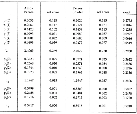
Perros rei error Snvder rei error exact

PI(0) 0.3055 0.118 0.3020 0.165 0.2733

PI(1) 0.2062 0.117 0.2124 0.151 0.1846

Pt(2) 0.1420 0.102 0.1434 0.113 0.1288

pl(3) 0.0993 0.071 0.0980 0.057 0.0927

pI(4) 0.0701 0.022 0.0680 0.009 0.0686

Pl(S) 0.0499 0.039 0.0479 0.077 0.0519

L

₁ 2.4069 0.269 2.4072 0.270 3.2960

P2(0) 0.3723 0.025 0.3724 0.025 0.3632 p2(1) 0.2560 0.030 0.2571 0.034 0.2486 p2(2) 0.1744 0.010 0.1740 0.008 0.1726

p2(3) 0.1973 0.085 0.1966 0.088 0.2156

L₂ 1.1967 0.035 1.1947 0.037 1.2406 P3(0) 0.5799 0.001 0.5800 0.000 0.5802 p3(1) 0.2485 0.003 0.2484 0.002 0.2478 p3(2) 0.1716 0.002 0.1715 0.003 0.1720

L3 0.5917 0.000 0.5915 0.001 0.5918

Table 3: 1\

=

1.20; ~

=

(2, 1, 2);

!!

=

(00 3, 2);

Altiok _Perros

Perros reI error Snyder rei error exact

P1(O) 0.1261 0.170 0.1248 0.158 0.1078

Pl (1) 0.1096 0.158 0.1111 0.174 0.0946

pl(2) 0.0956 0.144 0.0961 0.150 0.0836

pl(3) 0.0835 0.124 0.0833 0.121 0.0743

PI(4) 0.0731 0.104 0.0724 0.094 0.0662

PI(5) 0.0639 0.079 0.0632 0.068 0.0592

L

₁ 6.9948 _{0.188 6.9683 0.191 8.6170}

P2(O) 0.6489 0.041 0.6490 0.042 0.6231

p2(1) 0.2294 0.045 0.2311 0.037 0.2401

p2(2) 0.0818 0.110 0.0805 0.124 0.0919

p2(3) 0.0399 0.111 0.0395 0.120 0.0449

L₂ 0.5127 0.082 0.5104 0.086 0.5586

P3(0) 0.4560 0.000 0.4561 0.000 0.4563

p3(l) 0.2608 0.028 0.2608 0.028 0.2684 p3(2) 0.2832 0.029 0.2831 0.028 0.2753

L₃ 0.8272 0.010 0.8271 0.010 0.8190

I

Table s: X. = 0.8; ~ =(1,1,1); N = (00 3,2);

-

-rIO = 0.2, _{r 12} = 0.4, '13 = 0.4, '20

=

0.3, r23 = 0.7;

Altiok Perras

Perros rei error Snyder reI error exact

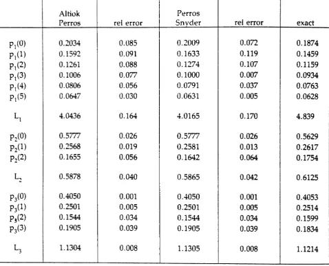
Pt(O) 0.2034 0.085 0.2009 0.072 0.1874

PI(1) 0.1592 0.091 0.1633 0.119 0.1459 pl(2) 0.1261 0.088 0.1274 0.107 0.1159 Pt(3) 0.1006 0.077 0.1000 0.007 0.0934 pl(4) 0.0806 0.056 0.0791 0.037 0.0763

P₁(S) 0.0647 0.030 0.0631 0.005 0.0628

L₁ 400436 0.164 4.0165 0.170 4.839

P2(0) 0.5777 0.026 0.5777 0.026 0.5629 p2(1) 0.2568 0.019 0.2581 0.013 0.2617

p2(2) 0.1655 0.056 0.1642 0.064 0.1754

L₂ 0.5878 00040 0.5865 0.042 0.6125 P3(0) 0.4050 0.001 0.4050 0.001 0.4053 p3(1) 0.2501 0.005 0.2501 0.005 0.2514

p3(2) 001544 0.034 001544 0.034 0.1599

p3(3) 0.1905 0.039 0.1905 0.039 0.1834

L₃ 1.1304 0.008 1.1305 0.008 1.1214

Table 5: A = 0.7; J.L =(1, .7, .8); LV

=

(00,2,3);

-

Altiok Perras

Perras reI error Snyder rei error exact

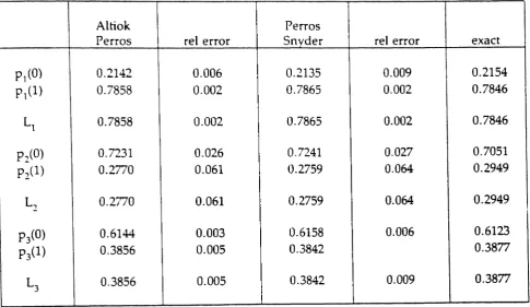
Pl(0) 0.2142 0.006 0.2135 0.009 0.2154

Pl(1) 0.7858 0.002 0.7865 0.002 0.7846

L₁ 0.7858 0.002 0.7865 0.002 0.7846

pz(O) 0.7231 0.026 0.7241 0.027 0.7051

p2(1) 0.2770 0.061 0.2759 0.064 0.2949

L., 0.2770 0.061 0.2759 0.064 0.2949

P3(O) 0.6144 0.003 0.6158 0.006 0.6123

p3(1) 0.3856 0.005 0.3842 0.3877

L₃ 0.3856 0.005 0.3842 0.009 0.3877

Table 6: A

=

3.0; ~=(1, 1, 1); N

=

(1 , 1, 1);

-

-rIO = 0.2, _{r 12}

=

0.4, r13

=

0.4, r20

=

0.5, r23

=

0.5;

Altiok Perros

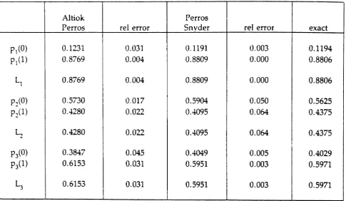
Perros reI error Snvder reI error exact

Pl(O) 0.1231 0.031 0.1191 0.003 0.1194

PI(1) 0.8769 0.004 0.8809 0.000 0.8806

L

₁ 0.8769 0.004 0.8809 0.000 0.8806

p~(O) 0.5730 0.017 0.5904 0.050 0.5625

p2(1) 0.4280 0.022 0.4095 0.064 0.4375

L

₂ 0.4280 0.022 0.4095 0.064 0.4375

P3(0) 0.3847 0.045 0.4049 0.005 0.4029

p3(1) 0.6153 0.031 0.5951 0.003 0.5971

L

₃ 0.6153 0.031 0.5951 0.003 0.5971

Table 7: A

=

500; ~=(1, 1, 1); N

=

(1, 1, 1);

-

-rIO = 0, r 12

=

0.5, r 13

=

0.5, r 20

=

0, r23

=

1;

Altiok _Perros

Perros rei error Snyder _{reI error exact}

Pl(O) 0.2262 _{0.126 0.2134 0.022}

0.2088 PI (1) 0.2081 0.052 0.2140 0.081 0.1979

P₁(2) 0.1948 0.024 0.1999 0.002 0.1996

PI(3) 0.1841 0.089 0.1878 0.014 0.2021 PI(4) 0.1868 0.064 0.1849 0.074 0.1996

L_I 1.8972 0.052 1.9168 0.042 2.0018

P2(O) 0.3257 0.056 0.3239 0.050 0.3084

p2(1) 0.2491 0.034 0.2510 0.026 0.2578

pz(2) 0.1868 0.052 0.1866 0.053 0.1970

p2(3) 0.2384 0.007 0.2385 0.007 0.2368

L₂ 1.3379 0.018 1.3397 0.062 1.3622 P3(O) 0.3900 0.023 0.3887 0.026 0.3990

P3(1) 0.2567 0.025 0.2565 0.026 0.2633

p3(2) 0.3533 0.046 0.3548 0.051 0.3377

L

₃ 0.9633 0.026 0.9661 0.029 0.9387

Table 8: A= 1.5; 1-1=(2,1,2); N = (4, 3.2);

-

-rIO = 0, r₁₂

=

0.5, _{r 13} = 0.5, r20 = 0, r23 = 1.0;

Altiok Perras

Perras rei error Snvder rei error exact

Pl(O) 0.0000 0.000 0.0000 0.000 0.0000 PI (1) 0.0001 0.000 0.0000 0.000 0.0001 pI(2) 0.0003 0.182 0.0006 0.455 0.0011

pl(3) 0.0110 0.078 0.0080 0.216 0.0102

pl(4) 0.0966 0.004 0.1002 0.042 0.0962 PI(5) 0.9810 0.002 0.8911 0.001 0.8924

L₁ 4.8777 0.000 -i.8816 0.000 4.8797 P2(0) 0.2800 0.001 0.2815 0.041 0.2705 p2(1) 0.2211 0.002 0.2225 0.009 0.2206

p2(2) 0.1737 0.016 0.1735 0.018 0.1766

p2(3) 0.1361 0.025 0.1353 0.031 0.1396

P2(4) 0.1821 0.055 0.1872 0.027 0.1924

L2 1.7052 0.033 01.7242 0.022 1.7634

P3(0) 0.4068 0.017 0.4080 0.014 004139 p3(1) 0.2502 0.002 002504 0.003 0.2496 p3(2) 0.1540 0.025 0.1537 0.028 0.1581

p3(3) 0.1890 0.059 0.1879 0.053 0.1784

L₃ 1.1252 0.022 1.1215 0.019 1.101

Table 9: 'A = 8.0; ~=(1, .5, 1); N= (5,4,3);

-

Altiok _Perros

Perros rei error Snyder _{reI error exact}

P1(0) 0.0233 0.387 _{0.0194 0.155 0.0168}

PI

(1) 0.0425 0.225 0.0389 0.124 0.0347

pl(2) 0.0773 0.087 _{0.0739 0.039 0.0711}

pl(3) 0.1407 0.013 0.1400 0.018 0.1425

Pi (4) 0.2558 0.062 0.2655 0.027 0.2728

Pl(S) 0.4604 0.004 0.-1622 0.000 0.4621

L

₁ 3.9444 0.015 3.9800 0.007 4.0061

P2(O) 0.6881 0.017 0.6456 0.019 0.6336

p2(1) 0.3559 0.029 0.3544 0.023 0.3664

L₂ 0.3559 0.029 0.3544 0.033 0.3664

P3(0) 0.4496 0.004 0.4516 0.000 0.4516

p3(1) 0.2607 0.056 0.2607 0.056 0.2761

p3(2) 0.2897 0.064 0.2877 0.056 0.2724

L₃ 0.8401 0.019 0.8361 0.015 0.8209

Table 10: A = 3.0~ J.L=(2,2,2); N

=

(5, 1,2);

-

-rIO = 0.2, r12

=

0.4, r13 = 0.4, '20 = 0.3, '23 = .7;

Altiok Perros

Pcrros rei error Snyder rei error exact

Pl(0) 0.1321 0.047 0.1261 0.001 0.1260

Pl(1) 0.8679 0.007 0.8739 0.000 0.8739

L₁ 0.8679 0.007 0.8739 0.000 0.8739

p~(O) 0.6978 0.037 0.7154 0.065 0.6727

p:!(I) 0.3022 0.077 0.2846 0.130 0.3273

L., 0.3022 0.077 0.2846 0.130 0.3773

P3(0) 0.7254 0.037 0.7273 0.039 0.6998

p3(1) 0.2746 0.085 0.2727 0.092 0.3002

L₃ 0.2746 0.085 0.2727 0.092 0.3002

P4(0) 0.3947 0.065 0.4219 0.001 004221

p4(1) 006053 0.047 0.5781 0.000 0.5779

I

Ly 0.6053 0.047 0.5781 0.000 0.5779

Table 11: A = .5; f.L=(1,1, 1, 1); N = (1,1,1,1);

-

--r10

=

0.05, r12 = 0.35, r13

=

0030, r14

=

0.30, r20 = 0.05, r23

=

.05; r24 = 0.90,

'30

=

0.05, r34 = 0.95:

Altiok _Perras

Perras rei error Snvder _{rei error exact}

PI(0) 0.3513 _{0.016 0.3439 0.005 0.3457}

PI (1) 0.6487 0.009 0.6560 0.003 0.6543

L₁ 0.6487 0.009 0.6560 0.003 0.6543 Pl(O) 0.7737 0.024 0.7795 0.032 0.7553

pz(l) 0.2263 0.075 0.2205 0.099 0.2447

L₂ 0.2263 0.075 0.2205 0.099 0.2447

P3(0) 0.7945 0.024 0.7931 0.022 0.7759

p3(1) 0.2056 0.083 0.2069 0.077 0.2241

L) 0.2056 0.083 0.2069 0.077 0.2241

P4(O) O.SliO 0.015 0.5271 0.005 0.5246

P4(1) 0.4830 0.016 0.4729 0.005 0.4754

L_y 0.4830 0.016 0.4729 0.005 0.4554

Table 12: A

=

3; ....

=

(2, 2, 2, 2); LV

=

(1, 1, 1, 1);

--

--rIO = 0.05, _{r 12} = 0.35, r 13 = 0.30. r 14

=

0.30, r20

=

0.05, '23 = .05; r24

=

0.90,

r30 = 0.05, r34 = 0.9,5;

Altiok Perros

Perros reI error Snyder rei error exact

Pl (0) 0.0246 00183 000174 00163 000208

Pl(1) 001405 00026 0.1448 00057 0.1370

pl(2) 008349 0.009 0.8379 00005 0.8422

L

₁ 108103 0.006 1.8205 0.001 1.8214

P2(O) 0.6266 0.044 0.6371 0.062 0.6001

p2(1) 0.2391 0.093 0.2405 0.088 002636

p2(2) 0.1363 00000 0.1225 0.101 0.1363

L., 005117 0.046 0.4854 0.095 0.5362

P3(0) 0.6605 0.047 0.6618 0.049 0.6311

p3(1) 0.2228 0.120 0.2267 0.105 0.2533

p3(2) 0.1167 00010 0.1115 0.035 0.1156

L₃ 004562 0.058 004497 00072 0.4845

P₄(0) 0.2429 0.121 002570 00070 002764

p

4(1) 002056 0.156 0.2114 0.132 0.2436

p4(2) 0.5515 0.149 005316 0.108 0.4800

Ly 103086 0.105 1.2746 0.059 1.2036

Table 13: A

=

5; f.L=(1, 1,1, 1); J.V

=

(2,2,2,2);

-

-rIO

=

0.05, r12

=

0.3.5, r13

=

0.30, r14

=

0.30, r 20

=

0.0.5, r₂₃

=

.05; r₂₄

=

0.90,

r30

=

0.05, r34 = 0095;

Altiok _Perras

Perras rei error _{Snvcier reI error exact}

Pl(O) 0.0232 0.326 _{0.0151 0.137 0.0175}

PI(1) 0.1359 0.057 0.1395 0.085 0.1286 pl(2) 0.8409 0.015 0.8454 0.010 0.8539

L

₁ 1.8177 0.010 1.8303 0.003 1.8364

P2(O) 0.6097 0.075 0.6254 0.102 0.5673 P2(1) 0.2447 0.118 0.2453 0.115 0.2773

p2(2) 0.1456 0.063 0.1294 0.167 0.1554

L₂ 0.5359 0.089 0.5040 0.143 0.5881

P3(O) 0.6450 0.078 0.6499 0.086 0.5983 p3(1) 0.2283 0.151 0.2316 0.138 0.2688 p3(2) 0.1267 0.047 0.1185 0.108 0.1329

L

₃ 0.4817 0.099 0.4686 0.123 0.5346

P₄(O) 0.2705 0.179 0.2914 0.116 0.3298

P₄(1) 0.7295 0.088 0.7086 0.159 0.6702

L_y 0.7295 0.088 0.7086 0.057 0.6702

I

Table 14: A. = 5; J..L=(1, 1, 1, 1); N = (2,2,2,1);

-

-rIO = 0.05, r12

=

0.30, _{r 13}

=

0.30, r20

=

0.05, r30 = 0.05, r34 = 0.95;

AP CPU = 0.87 min, PS CPU == O. 82 sec.

1

Pcrros ;

Snyder rei error simulation

Pt(O) O.~Q2 0.002 n.-tlJ3 p,(I) 0.250 0.000 0.250

P t(2) 0.127 0.008 0.128

p,(3) 0.064 0.000 U.064

p,(4) 0.033 0.000 0.033

pt(5) O.Oli 0.000 O.Oli

L_t 1.019 0.079 1.027

P2(0) 0.899 0.001 0.898

p:!(l) 0.091 0.000 0.091 P₂₍₂₎ 0.010 0.091 0.011

L.. 0.111 0.027 0.114

p)(O) 0.899 0.002 0.897 p)(l) 0.091 0.022 0.093 p3(2) 0.010 0.000 0.010

L) 0.111 0.018 0.113

p-\(O) 0.793 0.005 0.797

p-\(l) 0.164- 0.012 0.162

p-\(2) 0.043 0.024 0.042 L-\ 0.249 0.016 0.245

p,(O) 0.798 0.004 0.795 p,{l) 0.162 0.018 0.165 p,(2) 0.040 0.000 0.040 L__~ 0.242 0.012 0.245

Pb(O) 0.889 0.003 0.886

p₆(1) 0.099 0.020 0.101

p₆(2) 0.012 0.077 0.013 L₆ 0.123 0.031 0.127

P;(O) 0.i86 0.004 0.i89

p.tl) 0.168 0.006 0.169 p;(2) 0.045 o.on 0.042 L_ 0.259 0.024- 0.2.53

P8(O) 0.750 0.001 O.iSl

P9(1) 0.188 0.005 0.187

p~(2) 0.062 0.000 0.062

L~ 0.312 0.007 II 0.310

Table 15:

A = 1.0; J.L = (:rJ, 2,2,2,2,2,2,2,4); N =(~,2,2,2,2,2,2,2);

-

-rIO = 0, r12 =0.2, r13 = 0.2, r14 = 0.2, r 17 = 0.2, r18 =0.2,

r20 = 0, r24 = 0.5, r26 =0.5,

r30 =0, r34 = 0.5, '37 = 0.3,

r40 =0, r45 = 1.0,

r60 = 0, r56 =0.3, r57 = 0.3, r58 .= O...J.,

r60 = 0, r68 = 1.0,

r70 = 0, r78 = 1.0,

r80 = 1.0, PS Cf'U .= .05 sec

I Perros

I Snyder rei error simulation PI(O) I 0.403 0.189 0.339 PI( 1) 0.239 0.172 0.204 p,(2) 0.135 0.047 0.129 pl(3) 0.079 0.092 0.087 PI(4) 0.047 0.230 0.061 Pl(5) 0.030 0.333 0.045

L₁ 2.194 0.107 2.458

P2(0) 0.788 0.033 0.763 p2(1) 0.168 0.067 0.180 p:!(2) 0.044 0.228 0.057

L₂ 0.256 0.129 0.294

p)(O) 0.782 0.043 0.750

pJ{l) 0.172 0.090 0.189

p3(2) 0.046 0.025 0.061

L_J 0.264 0.154 0.312

P4(0) 0.547 0.036 0.528

p,,(I) 0.254 0.004 0.253

p,,(2) 0.200 0.005 0.219

L" 0.653 0.056 0.692

P5(0) 0.579 0.079 0.535 Ps(1) 0.258 0.019 0.263 Ps(2) 0.164 0.188 0.202

L_s 0.585 0.124 0.668

P6(0)

o.no

0.039 0.741

p₆(1) 0.178 0.082 0.194 p6(2) 0.052 0.200 0.065

L_o 0.282 0.127 0.323

P7(0) 0.543 0.034 0.525 p;(l ) 0.253 0.035 0.261 p;(2) 0.204 0.047 0.215 L_ _{0.661 0.042 0.690}

pg(O) 0.500 0.006 0.497 Ps(l) 0.252 0.109 0.257

p~(2) 0.248 0.012 0.245

Lq 0.i48 0.000 0.i48

Table 16:

k=2.0; J..L= ,(4,2,2,2,2,2,2,4);

N=(x,2,2,2,2,2,2,2);

! Pcrros ! _!

I

Snvdcr rei error I -rrnularion

P,(O) 0.487 0.002 O.4R6 p,(l) O.:!30 0.012 O.:!47 p,(2) 0.127 U.ooo 0.127 p,(3) 0.063 0.000 0.063 p,(4) 0.0..."4 U.030 'l.033

pt(5) 0.017 0.105 0.019

t, I.U55 0.030 1.088

p:(O) 0.799 0.005 n.i95 p:(l ) 0.161 0.006 0.162

p~(2) 0.032 0.059 0.034 p:(3) 0.008 0.111 0.009

L 0.149 0.027

! 0.236

P3(0) 0.797 0.009 i 0.790

I

p)(l) 0.162 0.024 I 0.166

P_J(2) 0.033 0.000 0.033

P3(3) 0.008 0.272 0.011

~ 0.252 0.049 0.165

P₄₍₀₎ 0.798 0.000 0.798 p4(1) 0.161 0.000 0.161

P4(2) 0.032 0.000 0.032 P4(3) 0.008 0.000 0.008

L-1 0.251 0.000 0.231

Ps(O) 0.796 0.009 0.789

P_s(l) 0.163 0.018 0.166

ps(2) 0.033 0.083 0.036

Pc;(3) 0.009 0.100 0.010 L_s o .,--.~~ 0.049 0.268

P6(0) 0.780 0.006 0.n5 P&(1 ) 0.172 0.006 0.173 p,,(2) 0.038 0.050 0.040 p,,(3) 0.011 0.083 0.012

L₆ 0.279 0.035 0.289

I

p_(O)

I 0.379 0.010 0.385

P;(1) 0.245 0.000 i 0.245

p,(2) 0.103 0.010 0.102 p;(3) O.Oi3 0.072 0.069

L 0.670 0.023 0.634

p~(O) 0.750 0.004 0.75) p~(l) 0.188 _I o.oi- 0.183 I

p~(2) 0.047 0.022 0.046 P3(3) o.or- 0.067 0.015

L~ 0.328 0.013 o~23

Table 17'

>"=1.0; ~=(3,1,1,2,2,1,1,~,; lV=(~,3,3,3,3,J,3..3l;

-

-routing as in table 15; PS CPU 0.09 sec

I

Perros ,

i Snyder rei error simulation

Pt(O)

I

0.262 1.647 0.099

PI(1 ) 0.191 1.690 0.071

Pt(2) 0.129 1.304 0.056

pt(3) 0.090 0.875 0.048 p,(4) 0.065 0.585 0.041

PI(S) 0.048 0.297 0.037 i, 14.39 0.162 17.17

P,(U) O.tJ56 0.068 0.614

p~(l) 0.233 0.009 0.235 p:(2) 0.110 0.272 0.151

i, 0.454 0.155 0.537

p)(O) 0.656 0.081 0.607

p:;(l) 0.233 0.045 0.244

p_J(2) 0.111 0.255 0.149 L_J 0.455 0.161 0.542

P4(0) 0.618 0.092 0.566

P..(1) 0.239 0.004 0.240

P.{Z) 0.143 0.267 0.195

LJ 0.526 0.164 0.629

p~(O) 0.600 0.302 0.461

Ps(1) 0.250 0.046 0.262

p:;(2) 0.150 0.440 0.277 L₅ 0.550 0.327 0.817

P6(0) 0.595 0.207 0.493

P6(1) 0.249 0.117 0.282

p_rt(2) 0.156 0.304 0.224

L₆ 0.561 0.233 0.731

P;(O) 0.471 0.163 0.405

pi(l) 0.273 0.000 0.273 p;(2) 0.256 0.205 0.322

L 0.785 0.144- 0.917

p~(O) 0.200 0.010 0.202 p,(l) O.ln 0.063 0.189 p,(2) 0.623 0.023 0.609

t, 1.423 I 0.011 1.407 Table18:

A=1.6; J.L=(3,1,1,2.2,1,2,2); N=(x,2,2,2,2,2,2,2);

-

Perras

Snvder rei error simulation

pt(O) 0.386 0.008 0.383

p,(l) 0.327 0.058 0.309

p_t(2) 0.288 0.065 0.308

L, 0.902 0.025 0.925

p:!(O) 0.704 0.000 0.704

p2(1) 0.213 0.009 O.:!15

p2(2) 0.088 0.086 0.081

~ 0.379 0.005 0.377

PJ(O) 0.b92 0.030 0.672

PJ{1) 0.218 0.056 0.231

p3(2) 0.090 0.072 0.097

L₃ 0.398 0.064 0.425

p~(O) 0.681 0.004 0.684

p..(l) 0.218 0.018 0.222

p4(2) 0.101 0.075 0.094

L~ 0.420 0.024 0.410

Ps(O) 0.674 0.043 0.646

Ps(1) 0.224 0.043 0.234

Ps(2) 0.103 0.134 0.119

L_s 0.429 0.093 0.473

P6(0) 0.683 0.004 0.686

p6(1) 0.218 0.009 0.220

P₆(2) 0.098 0.043 0.094

L_o 0.4:15 0.017 0.408

p:-(O) 0.390 0.042 0.407

p;(l) 0.249 0.095 0.275

p_(2) 0.361 0.132 0.319

L 0.971 0.065 0.912

p~(O) 0.644 0.012 0.652

P8(1) 0.230 0.013 0.233

p~(2) 0.127 0.95 0.116

L~ 0.483 0.041 0.464

Table 19:

A=2.0; ~=(3, 1,1,2,2, 1,1,.t); N=(2,2,2,2,2,2,2,2);

-

-routing same as in table 15; PS CPU 0.22 sec

Perros I

Snyder rei error simulation I

Pl(O) 0.362 0.014 0.357

!

pl(l) 0.334 0.031 0.324

i

p,(2) 0.304 0.044 0.318 I

I

L] 0.942 0.020 0.961 I

I

i

P2(O) 0.777 0.010 0.769

p2(1) 0.175 0.044 0.183

p2(2) 0.049 0.043 0.047

~ 0.272 0.022 0.278

P3(O) 0.770 0.016 0.758

!

p)(1) 0.179 0.058 0.190 _I

p)(2) 0.051 0.019 0.052

L) 0.281 0.044 0.294

P4(0) 0.521 0.017 0.530

p4(1) 0.257 0.059 0.273

p4(2) 0.222 0.127 0.197

L-1 0.701 0.051 0.667

Ps(O) 0.557 0.047 0.532

ps(l) 0.263 0.040 0.274

P_s(2) 0.180 0.072 0.194

Ls 0.623 0.059 0.662

P6(O) 0.759 0.017 0.746

p6(l) 0.184 0.061 0.196

p6(2) 0.057 0.017 0.058

L₆ 0.297 0.048 0.312

I

I

pj(O) 0.519 0.006 0.516

p,(l) 0.256 0.069 0.275

P7(2) 0.226 0.087 0.208

L, 0.707 0.022 0.692

P8(0) 0.478 0.020 0.488

p8(1) 0.252 0.056 0.267

p₈₍₂₎ 0.270 0.102 0.245

L~ 0.i92 0.045 0.758

Table 20:

A==3.0; J.L=(4,2,2,2,2,2,2,4); N = (2,2,2,2,2,2,2,2);

-

Pcrros I

Snvdcr rei error simulation p,(O) 0.323 0.006 0.321 p,(1 ) 0.335 0.073 0.313 p,(2) 0.342 0.066 0.366

L, 1.019 0.024 1.044

P₂(O) 0.593 0.013 0.601 P₂₍₁) 0.254 0.000 0.254

P2(2) 0.153 0.048 0.146

L₂ 0.560 0.028 0.545

P3(O) 0.587 0.005 0.584 p)(l) 0.256 0.019 0.261

p3(2) 0.157 0.013 0.155

L) 0.5i1 0.000 0.571

P₄(0) 0.551 0.023 0.564 p.,(l) 0.253 0.019 0.258 p4(2) 0.196 0.101 0.178

L₄ 0.645 0.050 0.614

Ps(O) 0.579 0.039 0.557 Ps(l) 0.258 0.030 0.266 Ps(2) 0.163 0.Oi9 0.177

L__~ 0.585 0.057 0.620

P₆₍₀₎ 0.768 0.024 0.750 P6(1 ) 0.180 0.077 0.195 p₆₍₂₎ 0.053 0.054 0.056

L₆ 0.286 0.065 0.6206

p;(O) 0.529 0.019 0.539 p;(l ) 0.254 0.059 0.270

p;(2) 0.216 0.131 0.191

L_ 0.687 0.052 0.306 I

I

I

I

0.436 0.046 0.-i5i

p~(O)

Ps(l) 0.250 0.046 0.262

p~(2) 0.314 0.125

I

0.281

L₈ 0.878 0.824 0.066

Table 21: ~=3.0; J.L =(4,1,1,2,2,2,2,3.5);

N = (2,2,2,2,2,2,2,2);

r~utingsame as in table 15; PS CPU =5.49 sec.

I Petros

ISnvdcr rei error simulation

I •

I

P,(O) 0.334 0.004 0.352

p,(l) 0.446 0.005 0.448 L, 0.446 0.005 0.448

P₂(O) O.fthA 0.009 0.6fiO

p=(1 ) 0.124 0.056 0.237

P₂₍₂₎ 0.075 0.014 O.Oi4

P2(3) 0.034 0.133 0.030

L~ 0.4n 0.006 0.474

p)(O) I 0.663 0.002 0.666

p)(l) 0.225 0.039 0.234

pJ(2) 0.076 0.041 0.073

p)(3) 0.034 0.214 0.028

L) 0.479 0.O3~ 0.463

P.•(O) 0.659 0.003 0.661

p,,(1) 0.225 0.043 0.235

P4(2) 0.077 0.041 0.074

p~(3) 0.038 0.267 0.030

L₄ 0.497 0.049 0.474

Ps(O) 0.663 0.008 0.658

P3(1) 0.225 0.034 0.233

p3(2) 0.076 0.013 0.077 P_s(3) 0.035 0.094 0.032

L₃ 0.483 0.000 0.483

P~(O) 0.813 0.007 0.807 p,,{l) 0.152 0.044 0.139

pP)

I

0.028 0.000 0.028

p,,(3) 0.007 0.167 0.006

L" 0.228 0.026 0.234

P7(0) 0.637 0.000 0.637

p;(1 ) 0.232 0.040 0.242

Pi(2) 0.084 0.000 0.084 p:-(3l 0.047 0.132 0.038

L 0.342 0.036 0.323

P~(O) 0.325 0.000 0.325

p~(1) 0.250 0.046 0.262

p~(2) O.11Q 0.033 0.123

p~(3l 0.106 0.191 0.OR9

L~ 0.803 0.037 0.776

Table 22: A=3.0; f..l=(-i,1,1,2,2,2,2,3.5);

Petros

Snyder reierror simulation

P,(O) 0.283 O.OOi 0.281 p, (1) 0.263 0.Oh5 0.247 p,(2) 0.229 0.013 0.226 p,(3) 0.224 0.089 0.246

L, 1.394 0.025 1.~3i

p~(O) 0.52i 0.015 0.535

P2(1) 0.258 0.012 0.261

P2(2) 0.125 0.025 0.122

P2(3) 0.090 0.098 0.082

L~ 0.7i9 0.036 0.752

p)tO) 0.520 0.004 0.522 p3(1) 0.259 0.008 0.261 p)(2) 0.127 0.008 0.128

P₃(3) 0.093 0.045 0.089

L) 0.795 0.014 0.784

P4(0) 0.499 0.014 0.506

p~(l) 0.254 0.004 0.255

p~(2) 0.127 0.031 0.131

p_~(3) 0.121 0.120 0.108

L-t 0.869 0.032 0.842

p,(O) 0.511 0.041 0.491 Ps(l) 0.260 0.008 0.262 p,(2) 0.130 0.044 0.136 p=;(3) 0.110 0.009 0.111 L__J 0.818 0.055 0.866

Pb(O) 0.727 0.028 0.707

P6(1) 0.200 0.061 0.213 P6(2) 0.054 0.115 0.061

p~(3) 0.020 0.000 0.020

Lr, 0.367 0.069 0.394

1 p_(O) 0.-148 0.013

! 0.4:54

I '

0.252 0.042

: p.tl) 0.263

p;(2) 0.140 0.054- 0.148 p_(3) 0.160 0.185 0.135 L_ 1.012 0.051 0.963

pg(O) 0.335 0.056 0.355

p_g(1) 0.228 0.050 0.240

p~(2) 0.155 0.055 n.lM

p~(3) 0.282

o.trs

0.240

L~ 1.384 0.074 1.289

:

Table 2.3: ".=3.0; J.L=(4,1,1,2,2,2,2,J.5);

~

Perros

! Snyder rei error simulation

P,(O) II 0.355 0.020 0.348

P.(1) 0.334 0.030 0.324 p,(2) 0.311 0.055 0.328

L, 0.956 0.025 0.980

P2(0) O.n8 0.004 0.775

P₂(1) 0.174 0.033 0.180 p:!(2) 0.048 0.066 0.045

L₂ 0.270 0.000 0.270

P3(O) 0.710 0.017 0.757 P3(1) 0.178 0.076 0.191 p)(2) 0.051 0.020 0.052

L) 0.281 0.047 0.295

p~(O) 0.523 0.032 0.540

p,,(l) 0.257 0.041 0.268

p,,(2) 0.220 0.146 0.192

L. 0.697 0.069 0.652

P5{O) 0.555 0.051 0.528 Ps(l) 0.264 0.040 0.275 p;(2) 0.182 0.076 0.197

L__, 0.669

P&(O) 0.755 0.029 0.734 P&(l) 0.186 0.084 0.203 P₆₍₂₎ 0.059 0.Oi8 0.064

L_b 0.304 0.079 0.330

P;(O) 0.500 0.002 0.499

p;(l) 0.256 0.086 0.280

p;(2) 0.243 0.100 0.221

L _I 0.743 0.026 0.722

P8(0) 0.409 0.038 0.425 Ps(l) 0.247 0.078 0.268

pg(2) 0.344 0.121 0.307 L~ I 0.935 0.059 0.883

Table 24: ~.. =3.0; fJ..=(4,2,2,2,2,2,2,3.5);

1'1=(2,2,2,2,2,2,2,2);

REFERENCES

(1) Altiok, T., "Approximate analysis of exponential tandem queues with blocking,"

Europ, /. Opere Res. 11 (1982) 390-398.

(2) Altiok, T., and H.G. Perros, "Open networks of queues with blocking: split and merge configurations," to appear in it\lIS Trans.

(3) Altiok, T., and H.G. Perras, "Approximate analysis of arbitrary configurations of open queueing networks with blocking," to appear in the Annals of OR.

(4) Bocharov, P.P. and G.P. Rokhas, "On an exponential queueing system in series with blocking," Problems of Control and Information Theory, 9 (1980), 441-455.

(5) Boxma, O.J. and A.G. Konheim, "Approximate analysis of exponential queue-ing systems with blockqueue-ing," Actalnlormaticai'» (1981) 19-66.

(6) Brandwajn, A. and Y.L. [ow "An approximate method for tandem queues with blocking,It manuscript, Amdahl Corp. (1985).

(7) Caseau, P. and G. Pujolle, 'Throughput capacity of a sequence of queues with blocking due to finite waiting room," IEEE Trans. Soft. Eng. 5£-5 (1979) 631-642. (8) Gershwin, S. B. "An efficient decomposition method for the approximate

evalua-tion of tandem queues with finite storage and blocking," manuscript, Lab. for

Information and Decision Sciences, MIT, (1983).

(9) Goto, K., Y. Takahashi, and

J.

Hasegawa, "An approximate analysis on con-trolled tandem queues," Proc. Modelling Techniques and Tools for Performance Analysis, June 1985, Cannes France.

(10) Hillier, F.S., and R. Boling, ''Finite queues in series with exponential or Erlang service times-A numerical approach," Opere Res. 15 (1967) 286-303.

(11) Hordijk, A. and N. Van Dijk, 'Networks of queues with blocking," Performance

'81, F.]. Kylstra (ed.) , North-Holland, New York (1981).

(12) Kelly, F.P., Reversibility and Stochastic Networks, New York, Wiley, 1979.

(13) Kelly, F.P. 'The throughput of a series of buffers," Adv. Appl. Prob., 14 (1982) 633-653.

(14) Labetoulle,

J.

and G. Pujolle, "Modelling of packet switching communication networks with finite buffer size at each node," Computer Periormance, Chandy

and Reiser (eds), North Holand (1977), 515-535.

(15) Le Ny. L.-M, "Etude analytique de reseaux de files d'attente multiclasses a routage variable," RAIRO Recherche Operaiionel!e. 14 (1980) 331-347.

(16) Onvural. R.O. and H.G. Perras, "On equivalencies of blocking mechanisms in queueing networks with bocking," to appear in Letters ofOR.

(18) Perras, H.G. and T. Altiok, "Approximate analysis of open networks of queues

with blocking: Tandem configurations,"

IEEE Trans. on

so«.

Eng.,

Vol. SE-12 (1986) 45-461.

(19) Perras, H.G. "A Survey of Queueing ~etworks with Blocking-Part I,"

Com-puter Science Report, N.C. State University 1986.

(20) Pollock, S.Nt., ].R. Birge and

1.M.

Alden, "Approximation analysis for open tan-dem queues with blocking: Exponential and general service distributions," manuscript, I. and OR Dept. 83-16, Michigan Univ. (1985).

(21) Suri, R. and G. W. Diehl, "A variable buffer-size model and its use in analytic closed queueing networks with blocking," Proc. ACM SIGMETRICS on Measure-mentand Modellingof Computer Systems, (1984), 134-142.

(22) Takahashi, Yo H. Miyahara and T. Hasegawa, "An approximation method for open restricted queueing networks,"

J.

Oper. Res. 28 (1980),594-602.

(23) Veran, M. and D. Potier, "QNAP2: A portable environment for queueing sys-tems modelling," INRIA Rep. 314 (1984).

(24) Yao, D. and J.A. Buzacott, "Modelling a class of flexible manufacturing systems