Volume 2007, Article ID 74243,13pages doi:10.1155/2007/74243
Research Article
Event Detection Using “Variable Module Graphs” for
Home Care Applications
Amit Sethi, Mandar Rahurkar, and Thomas S. Huang
Department of Electrical and Computer Engineering, University of Illinois at Urbana-Champaign, Urbana, IL 61801-2918, USA
Received 14 June 2006; Accepted 16 January 2007
Recommended by Francesco G. B. De Natale
Technology has reached new heights making sound and video capture devices ubiquitous and affordable. We propose a paradigm to exploit this technology for home care applications especially for surveillance and complex event detection. Complex vision tasks such as event detection in a surveillance video can be divided into subtasks such as human detection, tracking, recognition, and trajectory analysis. The video can be thought of as being composed of various features. These features can be roughly arranged in a hierarchy from low-level features to high-level features. Low-level features include edges and blobs, and high-level features include objects and events. Loosely, the low-level feature extraction is based on signal/image processing techniques, while the high-level feature extraction is based on machine learning techniques. Traditionally, vision systems extract features in a feed-forward manner on the hierarchy, that is, certain modules extract low-level features and other modules make use of these low-level features to extract high-level features. Along with others in the research community, we have worked on this design approach. In this paper, we elaborate on recently introduced V/M graph. We present our work on using this paradigm for developing applications for home care applications. Primary objective is surveillance of location for subject tracking as well as detecting irregular or anomalous behavior. This is done automatically with minimal human involvement, where the system has been trained to raise an alarm when anomalous behavior is detected.
Copyright © 2007 Amit Sethi et al. This is an open access article distributed under the Creative Commons Attribution License, which permits unrestricted use, distribution, and reproduction in any medium, provided the original work is properly cited.
1. INTRODUCTION
Even with the US population rapidly aging, a smaller pro-portion of elderly and disabled people live in nursing homes today compared to 1990. Instead, far more depend on as-sisted living residences or receive care in their homes [1]. Majority of people who need long-term care still live in nurs-ing homes, however the proportion of nursnurs-ing home beds declined from 66.7 to 61.4 per 10 000 population. Accord-ing to the author, these changAccord-ing trends in the supply of long-term care can be expected to continue because the de-mand for home- and community-based services is growing. These healthcare services besides being expensive may of-ten be emotionally traumatic for the subject. Large num-ber of these people who live here can perform basic day-to-day tasks, however need to be under constant supervision in case assistance is required. In this paper, we show how cur-rent technology can enable us to monitor these subjects in an environment which is most amicable—their own home. Today’s digital technology has made sound and video
cap-ture devices affordable for a common user. Also there has been tremendous progress in research and development in the fields of image and video compression, editing, and anal-ysis software leading to its effective usability and commer-cialization.
We elaborate on a recently proposed framework [2] based on factor graphs. It relaxes some of the constraints of the tra-ditional factor graphs [3] and replaces its function nodes by modified versions of some of the modules that have been de-veloped for specific vision tasks. These modules can be easily formulated by slightly modifying modules developed for spe-cific tasks in other vision systems, if we can match the input and output variables to variables in our graphical structure. It also draws inspiration from product of experts [4], and free energy view [5] of the EM algorithm [6]. We present some preliminary results for tracking and event detection applica-tions and discuss the path for future development.
Outline of this paper is as follows. Section 2 intro-duces factor graphs, thereby generalizing to variable mod-ule or V/M graphs inSection 3. V/M graphs are explored extensively, thus establishing the theoretical background in Section 4. We demonstrate use of V/M graphs for home care applications, especially complex event detection and subject tracking inSection 5.
2. ALGORITHMS
2.1. Factor graphs
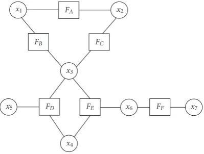
In order to understand V/M graphs, we briefly explain factor graphs. A factor graph is a bipartite graph that expresses a structure of factorization of a function into product of sev-eral local functions, thus making it efficient to represent the dependencies between random variables. Factor graph has a variable node for each random variablexi, factor node for each local function fj, and a connecting edge between vari-able nodexiand factor nodefjonly ifxiis an argument offj. A factor (function) of a product term can selectively look at a subset of dimensions while leaving the other dimensions that are not in the subset for others factors to constrain. In other words, only a subset of variables may be part of the constraint space of a given expert. This leads to the graphs structure of a factor graph, where the edges between a factor function node and variable nodes exist only if the variable appears as one of the arguments of the factor function,
px1,x2,x3,x4,x5
∝
⎛ ⎜ ⎜ ⎜ ⎝
pA
x1, x2, x3, x4, x5
× pB
x1, x2, x3, x4, x5
× pC
x1, x2, x3, x4, x5
× pD
x1, x2, x3, x4, x5
⎞ ⎟ ⎟ ⎟ ⎠
∝
⎛ ⎜ ⎜ ⎜ ⎝
fA
x1, x2
× fB
x2, x3
× fC
x1, x3
× fD
x3, x4, x5
⎞ ⎟ ⎟ ⎟ ⎠.
(1)
In (1), fA(x1,x2), fB(x2,x3), fC(x1,x3), and fD(x3,x4,x5)
are the factor functions of the factor graph. The factor graph in (1) can be expressed graphically as shown inFigure 1.
Inference in factor graphs can be made using a local mes-sage passing algorithm called the sum-product algorithm [3]. The algorithm reduces the exponential complexity of calcu-lating the probability distribution over all the variables into more manageable local calculations at the variable and
func-x1 FA x2
FB FC
x3
x5 FD
x4
Figure1: Example factor graph.
tion nodes. The local calculations depend only on the incom-ing messages from the nodes adjacent to the node at hand (and the local function, in case of function nodes). The mes-sages are actually distributions over the variables involved. For a graph without cycles, the algorithm converges when messages pass from one end of the graph to the other and back. For many applications, even when the graph has loops, the messages converge in a few iterations of message passing. Turbo codes in signal processing make use of this property of convergence of loopy propagation [7]. The message pass-ing clearly is a principled form of feedback or information exchange between modules. We will make use of a variant of message passing for our new framework because exact mes-sage passing is not feasible for complex vision systems.
3. V/M GRAPH
We develop a hybrid framework to design modular vi-sion systems. In this new framework, which we call vari-able/module graphsorV/M graphs[2,8], we aim to borrow the strengths of both modular and generative designs. From the generative models in general and probabilistic graphical models in particular, we want to keep the principled way to explain all the information available and the relations be-tween different variables using a graphical structure. From the modular design, we want to borrow ideas for local and fast processing of information available to a given module as well as online adaptation of model parameters.
3.1. Replacing functions in factor graphs with modules
many of the other graphical models can be converted to fac-tor graphs.
Modules in modular design take (probability distribu-tions of) various variables as inputs, and produce (probabil-ity distributions of) variables as outputs. Producing an out-put can be thought of as passing a message from the mod-ule to the output variable. This is comparable to part of the message passing algorithm in factor graphs, that is, passing a message from the function node to a variable node. This cal-culation is done by multiplying messages from all the other variable nodes (except the one that we are sending the mes-sage to) to the factor function at the function node, and marginalizing the product over all the other variables (ex-cept the one that we are sending the message to). Processing of a module can be thought of as an approximation to this calculation.
However, the notion of a variable node does not exist in modular design. Let us, for a moment, imagine that modules are not connected to each other directly. Instead, let us imag-ine that every connection that connects output of a module to the input of another module is replaced by a node con-nected to the output of the first module and input of the sec-ond module. This node represents the output variable of the first module, which is the same as the input node of the sec-ond module. Let us call this thevariable node.
In other words, a cascade of modules in a modular sys-tem is nothing but a cascade of approximations to function nodes (separated by variable nodes, of course). If we gen-eralize this notion of interconnection of module ormodule nodesvia variable nodes, we get a graph structure. We refer to his bipartite graph asvariable/module graph. Thus, if we replace the function nodes in a factor graph by modules, we get a variable/module graph—a bipartite graph in which the variables represent one set of nodes (called variable nodes), and modules represent the other set of nodes (called module nodes).
4. SYSTEM MODELING USING V/M GRAPHS
A factor graph is a graphical representation of the fac-torization that a product form represents. Since the vari-able/module graph can be thought of as a generalization of the factor graph, what does this mean for the application of product form to the V/M graph? In essence, we are still mod-eling the overall constraints on the joint-probability distri-bution using a product form. However, the rules of message passing have been relaxed. This makes the process an approx-imation to the exact product form [8]. To see how we are still modeling the joint-distribution over the variables using a product form, let us start by analyzing the role of modules. A module takes the value of the input variable(s)xiand pro-duces a probability distribution over the output variable(s) xj. This is nothing but the conditional distribution over the output variables given the input variable, orp(xj|xi). Thus, each module is nothing but an instantiation of such condi-tional density functions.
In a Bayesian network, similar conditional probability distributions are defined, with an arrow representing the
di-rection of causality. This makes it a simple case to define the module as a/an (set of) arrow(s) going from the input to the output, converting the whole V/M graph into a Bayesian net-work, which is another graphical representation of the prod-uct form. Also, since the Bayesian network can always be con-verted into a factor graph [9], we can convert a V/M graph into a factor graph. However, processing modules are many times arranged in a bottom-up fashion, whereas the flow of causality in a Bayesian network is top-down. This is not a problem, since we can use Bayes rule to reverse the flow of causality. Once we have established a module as an equiva-lent of a conditional density, manipulation of the structure is easy, and it always remains in the purview of product form modeling of the joint distribution. However, the similarity between V/M graphs and probabilistic graphical models ends here on a theoretical level. As we will inSection 4.1, the in-ference mechanisms that are applied in practice to graphical models are not applied in the exact same manner to V/M graphs. One of the reasons for this is that modules do not produce a functional form of the conditional density func-tions. They only produce a black box that we can sample out-put (distribution) from for given sample points of inout-put, and not the other way around. Thus, in practice, application of Bayes rule to change the direction of causality is not as easy as it is in theory. We use comodules, at times, for flow of mes-sages in the other direction to a given module.
4.1. Inference
as well. A way to do this is to associate a comodule with the module that does the reverse of the processing that the mod-ule does. For example, if a modmod-ule takes in a background mask and outputs probability map of the position of a hu-man in the frame, the comodule will provide some proba-bility map of pixels belonging to background or foreground (human) given the position of human to this comodule.
In case the module node is a deterministic function, the probability function of the output variable will be treated as a delta function. Although there are definite merits of a stricter definition of a V/M graph for a stringent mathemat-ical analysis, it might result in loss of applicability and flexi-bility to workable systems at this point. By introducing mod-ified modules as approximation to functions and their mes-sage calculation procedures, we get computationally cheap approximations to complex marginalization operations over functions that will be difficult to perform from first princi-ples or statistical sampling, the approach used with genera-tive models until now. Whether this kind of message passing will converge or not even for graphs without cycles remains to be seen in theory, however, we have found the results to be convincing for the applications that we implemented it for as shown inSection 5.
4.2. Learning
There are a few issues that we would like to address while de-signing learning algorithms for complex vision systems. The first issue is that when the data and system complexity are prohibitive for batch learning, we would really like to have designs that lend themselves to online learning. The second major issue is the need to have a learning scheme that can be divided into steps that can be performed locally at diff er-ent modules or function nodes. This makes sense, since the parameters of a module are usually local to the module. Es-pecially in an online learning scheme, the parameters should depend only on the local module and the local messages in-cident on the function node.
We will derive learning methods for V/M graphs based on those for probabilistic graphical models. Although meth-ods for structure learning in graphical models have been ex-plored [11, 12], we will limit ourselves for the time being to parameter learning. In line with our stated goals in the paragraph above, we will consider online and local param-eter learning algorithms for probabilistic graphical models [13,14] while deriving learning algorithms for V/M graphs.
Essentially, parameter adjustment is done as a gradient ascent over the log likelihood of the given data under the model. While formulating the gradient ascent over the cost function, due to the factorization of the joint-probability dis-tribution, derivative of the cost function decomposes into a sum of terms, where each term pertains to local functions. A similar idea can be extended to our modified factor graphs or V/M graphs.
Now, we will derive a gradient-ascent-based algorithm for parameter adjustment for V/M graphs. Our goal is to find the model parameters that maximize the data likelihood p(D), which is a standard goal used in the literature [6,13], since (observed) data is what we have and seek to explain,
while the rest of the (hidden) variables just aid in modeling the data. Each module will be represented by a conditional density functionpωi(xi |Ni). Here,xirepresents the output
variable of theith module,Nirepresents the input set of vari-ables to theith module, andωirepresents the parameters as-sociated with the module. We will make the assumption that data points are independently identically distributed (i.i.d.), which means that for data pointsdj (where j ranges from 1 tom, the number of data points) and the data likelihood p(D), (2) holds,
p(D)= m
j=1
pdj
. (2)
In principle, we can choose any monotonically increasing function of the likelihood, and we chose the ln(·) function to convert the product into a sum. This means that for the log likelihood, (3) holds,
lnp(D)= m
j=1
lnpdj
. (3)
Therefore, when we maximize the log likelihood with respect to the parametersωi’s, we can concentrate on maximizing the log likelihood of each data point by gradient ascent, and adding these gradients together to get the complete gradi-ent of the log likelihood over the gradi-entire data. Thus, at each step we need to deal with only one data point, and accumu-late the result as we get more data points. This is significant in developing online algorithms that deal with limited (one) data point(s) at a time. In case where we tune the parameters slowly, this is in essence like a running average with a forget-ting factor.
Now, taking the partial derivative of the log likelihood of one data pointdjwith respect to a parameterωi, we get
∂lnpdj
∂ωi = ∂/∂ωi
pdj
pdj
=
∂/∂ωi xi,Nip
dj|xi,Ni
pxi,Ni
dxidNi
pdj
=
∂/∂ωi xi,Nip
dj|xi,Ni
pxi|Ni
pNi
dxidNi
pdj
=
xi,Ni
∂/∂ωi
pdj|xi,Ni
pxi|Ni
pNi
dxidNi pdj
=
xi,Nip
Ni
∂/∂ωi
pdj|xi,Ni
pxi|Ni
dxidNi pdj
.
(4)
when we are not even expecting to calculate the gradient, we will only try to do a generalized gradient ascent by going in the direction of positive gradient. It suffices that as an ap-proximate greedy algorithm, we move in the general direc-tion of increasing p(xi | Ni) and hope that p(dj | xi,Ni), which is a marginalization of the product ofp(xk|Nk) over manyk’s, will follow an increasing pattern as we spread the procedure over many k’s (modules). The greedy algorithm should be slow enough in gradient ascent that it can cap-ture the trend over many j’s (data points) when run online. This sketches the general insight into the learning algorithm. The sketch is in line with a similar derivation for Bayesian network parameter estimation in [13], where the scenario is much better defined than it is for V/M graphs. InSection 4.4, we provide another viewpoint to justify the same steps.
4.3. Free-energy view of EM algorithm and V/M graphs
For generative models, the EM algorithm [6] and its on-line, variational, and other approximations have been used as the learning algorithm of choice. Online methods work by maintaining sufficient statistics at every step for theq -function that approximates the probability distributionpof hidden and observed variables. We use a free-energy view of the EM algorithm [5] to justify a way of designing learning algorithms for our new framework. In [5], the online or in-cremental version of EM algorithm was justified using a dis-tributed E-step. We extend this view to justify local learn-ing at different module nodes. Being equivalent to a varia-tional approximation to the factor graph means that some of the concepts applicable to generative models, such as vari-ational and online EM algorithms, can be applicable to the V/M graphs. We use this insight to compare inference and learning in V/M graphs to the free-energy view of EM algo-rithm [5].
Let us assume thatXrepresents the sequence of observed variablesxi, andY represents the sequence of hidden vari-ables yi. So, we are modeling the generative process p(xi | yi,θ), with some prior onyi;p(yi), given system parameters θ(which is the same for all pairs (xi,yi)). Due to the Marko-vian assumption ofxibeing conditionally independent ofxj givenY, wheni=j, we get
p(X|Y,θ)= i
pxi|yi,θ
. (5)
We would like to maximize the log likelihood of the ob-served dataX. EM algorithm does this by alternating between an E-step as shown in (6) and an M-Step shown in (7) in each iteration with iteration numbert,
compute distribution:qt(y)=py|x,θ(t−1), (6)
compute arg max:θ(t)=arg max
θ Eqt
logP(x,y|θ). (7)
Going by the free-energy view of the EM algorithm [5], the E- and M-steps can be viewed as alternating between maximizing the free energy with respect to the q-function
and the parametersθ. This is related to the minimization of free energy in statistical physics. The formulation of free en-ergyFis given in
F(q,θ)=Eq
log(x,y|θ)+H(q)= −Dqpθ
+L(θ). (8)
In (8),D(qp) represents the KL-divergence betweenq and pgiven by (9), andL(θ) represents the data likelihood for the parameterθ. In other words, the EM algorithm alter-nates between minimizing the KL-divergence betweenqand p, and maximizing the likelihood of the data given the pa-rameterθ,
Dqp=
yq(y) log q(y)
p(y)dy. (9)
The equivalence of the regular form of EM and the free-energy form of EM has already been established in [5]. Fur-ther, since yi’s are independent of each other, theq(y) and p(y) terms can be split into products of differentq(yi)’s and p(yi)’s, respectively. This is used to justify the incremental version of EM algorithm that incrementally runs partial or generalized M-steps on each data point. This can also be done using sufficient statistics of the data collected until that data point, if it is possible to define sufficient statistics for a sequence of data points.
Coming back to the message passing algorithm, for each data point, when message passing converges, the beliefs at each variable node give a distribution over all the hidden variables. If we look at theq-function, it is nothing but an approximation of the actual distribution over the variablep, and we are trying to minimize the KL-divergence between the two. Now, we can get the sameq-function from the con-verged messages and beliefs in the graphical model. Hence, one can view message passing as a localized and online ver-sion of the E-step.
4.4. Online and local M-step
One issue that still remains is the partition function. With all the local M-steps maximizing one term of the likelihood in a distributed fashion, it is likely that the local terms in-crease infinitely, while the actual likelihood does not. This problem arises when appropriate care is not taken to nor-malize the likelihood by dividing it with a partition func-tion. While dealing with sampling-based numerical integra-tion methods such as MCMC [15], it becomes difficult to cal-culate the partition function. This is because methods such as importance sampling and Gibbs sampling used in MCMC deal with surrogateq-function, which is usually a constant multiple of the targetq-function. The multiplication factor can be assessed by integrating over the entire space, which is difficult. There are two ways of getting around this problem. One way was suggested in [4] as maximizing the contrastive divergence instead of the actual divergence. The other way is to put some kind of local normalization in place while cal-culating messages sent out by various modules. As long as the multiplication factor of theq-function does not increase beyond a fixed number, we can guarantee that maximizing the local approximation of the components of the likelihood function will actually improve system performance.
In the M-step of the EM algorithm, we minimize Q(θ,θ(i−1)) with respect toθ. In the proof given by (10), we
show how this minimization can be distributed over different components of the parameter variableθ,
Qθ,θ(i−1)=Elogp(X,Y |θ)|X,θ(i−1)
=
h∈Hlogp(X,Y |θ)f
Y|X,θ(i−1)dh
=
h∈H
m
i=1
logpxi,yi|θi
fY |X,θ(i−1)dh
= m
i=1
h∈Hlogp
xi,yi|θi
fY|X,θ(i−1)dh,
(10)
M-step:θ(i)←−arg max θ Q
θ,θ(i−1). (11)
4.5. Probability distribution function softening
Until now, PDF softening was only intuitively justified [4]. In this section, we revisit the intuition, and justify the concept mathematically in
Dqp
=
x∈Xq(x) log q(x) p(x)dx
=
x∈Xq(x) logq(x)dx−
y∈Xq(y) logp(y)dy
=
x∈Xq(x)log
iqi(x)
w∈X
jqj(w)dwdx−
y∈Xq(y)logp(y)dy
=
x∈Xq(x)
i
logqi(x)
−log w∈X
j
qj(w)dw
dx
−
y∈Xq(y) logp(y)dy
=
x∈X
i
q(x) logqi(x)
−q(x) log
w∈X
j
qj(w)dw
dx
−
y∈Xq(y) logp(y)dy
=
i x∈X
q(x) logqi(x)dx
−
z∈Xq(z)log
w∈X
j
qj(w)dw
dz−
y∈Xq(y)logp(y)dy
=
i x∈X
q(x) logqi(x)dx
−log
w∈X
j
qj(w)dw
z∈Xq(z)dz−
y∈Xq(y)logp(y)dy
=
i x∈X
q(x) logqi(x)dx
−log w∈X
j
qj(w)dw
−
y∈Xq(y) logp(y)dy.
(12)
As shown in (12), if we want to decrease the KL-diver-gence between the surrogate distribution q and the actual distributionp, we need to minimize the sum of three terms. The first term on the last line of the equation is minimized if there is an increase in the high-probability region as de-fined byq, which is actually a low-probability region for an individual componentqi. This means that this term prefers diversity among differentqi’s, sinceqis proportional to the product ofqi’s. Thus, the low-probability regions ofqneed not be low-probability regions of a givenqi. On the other hand, the third term is minimized if there is an overlap be-tween the high-probability region as defined byq and the high-probability region defined by pand between the low-probability region as defined byq and the low-probability region defined byp. In other words, surrogate distributionq should closely model the actual distributionp.
an expert and being overcommitted to any particular solu-tion (high-probability region).
4.6. Prescription
With the discussion on the theoretical justification of the de-sign of V/M graphs complete, in this section we want to sum-marize how to design a V/M graph for a given application. In Section 5, we will present experimental results of successful design of vision systems for complex tasks using V/M graphs. To design a V/M graph for an application, we will follow the following guidelines.
(1) Identify the variables needed to represent the solution. (2) Identify the intermediate hidden variables.
(3) Suitably breakdown the data into a set of observed variables.
(4) Identify the processing modules that can relate and constrain different variables.
(5) Ensure that there is enough diversity in the processing modules.
(6) Lay down the graphical structure of the V/M graph similar to how one would do that for a factor graph, using modules instead of function nodes.
(7) Redesign each module so that it can tune online to increase local joint-probability function in an online fashion.
(8) Ensure that the modules have enough variance or le-niency to be able to recover from mistakes based on the redundancy provided by the presence of other mod-ules in a graphical structure.
(9) If a module has no feedback for a variable node, this can be considered to be a feedback equivalent of a uni-form distribution. Such a feedback can be dropped from calculating local messages to save computation.
Once the system has been designed, the processing will follow a simple message passing algorithm while each mod-ule will learn in a local and online manner. If the results are not desirable, one would want to replace some of the mod-ules with better estimators of the given task, or make the graph more robust by adding more (and diverse) modules, while considering making modules more lenient.
5. EXPERIMENTS
In this section, we report design and experimental results of several applications related to home care applications under the broad problem of automated surveillance. We focus on security and monitoring of home care subjects, and hence the targeted applications are automatic event detection and abnormal event detection. Thus, an alarm would be raised in case of abnormal activity, for example, like subject falling down. Event is a high-level semantic concept and is not very easy to define in terms of low-level raw data. This gap be-tween the available data and the useful high-level concepts is known as thesemantic gap. It can be safely said that the vi-sion systems, in general, aim to bridge the semantic gap in visual data processing. Variables representing high-level
con-x1 FA x2
FB FC
x3
x5 FD
x4
Figure2: V/M graph for single-target tracking application.
cepts such as events can be conveniently defined over lower-level variables such as position of people in a frame; provided that the defining lower-level variables are reliably available. For example, if we were to decide whether a person came out or went in through a door, we can easily decide this if the sequence of the position of the person (and the position of the door) in various frames in the scene was available to us. This is the rationale behind modular design, where in this case, one would devise a system for person tracking, and the output of the tracking module would be used by an event de-tection module to decide whether the event has taken place or not.
The scenario that we considered for our experiments is related to the broad problem of automated surveillance. Without loss of generality, we assume a fixed camera in our experiments. In the following experiments, we concentrate on several applications of V/M graphs in the surveillance set-ting. We will proceed from simpler tasks to increasingly com-plex tasks. While doing so, many times we will incrementally build upon previously accomplished subtasks. This will also showcase one of the advantages of V/M graphs; namely, easy extendability.
5.1. Application: person tracking
We start with the most basic experiment, where we build an application for tracking a single target (person) using a fixed indoor camera. In this application, we identify five variables that affect inference in a frame. The intensity map (pixel val-ues) of the frame (or, the observed variable(s)), the back-ground mask, the position of the person in the current frame, the position of the person in previous frame, the velocity of the person in previous frame. These variables are repre-sented asx1,x2,x3,x4, andx5, respectively inFigure 2. All
nodes exceptx1 are hidden nodes. The variables exchange
FArepresents the background subtraction module that main-tains an eigenbackground model [16] as system parameters, using a modified-version online learning algorithm for per-forming principal component analysis (PCA) as described in [17]. While it passes information from x1 to x2, it does
not pass it the other way round, as image intensities are evi-dence, hence fixed. ModuleFCserves as the interface between the background mask and the position of the person. In ef-fect, we run an elliptical Gaussian filter, roughly of the size of a person/target, over the background map and normalize its output as a map of the probability of a person’s position. ModuleFB serves as the interface between the image inten-sities and the position of the person in the current framex3.
Since it is computationally expensive to perform operations on every pixel location, we sample only a small set of po-sitions to confirm if the image intensities around that posi-tion resemble the appearance of the person being tracked. The module maintains an online learning version of eige-nappearance of the person as system parameters based on a modification of a previous work [18]. It also does not pass any message tox1. The position of the person in the current
frame is dependent on the position of the person in the pre-vious framex4and the velocity of the object in the previous
framex5. Assuming a first-order motion model, which is
en-coded inFDas a Kalman filter, we connectx3tox4andx5.x4
andx5are assumed fixed for the current frame, thereforeFD only passes the message forward tox3and does not pass any
message tox4orx5.
5.1.1. Message passing and learning schedule
The message passing and learning schedule used was as fol-lows.
(1) Initialize a background model.
(2) If a large contiguous foreground area is detected, ini-tialize a person detection module FC, and tracking-related modulesFBandFD.
(3) Initialize the position of the person in the previous frame as the most likely position according to the background map.
(4) Initialize the velocity of the person in the previous frame to be zero.
For every frame,
(1) propagate a message fromx1toFAas the image; (2) propagate a message fromx1toFBas the image; (3) propagate messages fromx4andx5toFD;
(4) propagate a message fromFDtox3in the form of
sam-ples of likely position;
(5) propagate a message from FA to x2 in form of a
background probability map after an eigenbackground subtraction;
(6) propagate a message from x2 to FC in the form of a background probability map;
(7) propagate a message from FC tox3 in the form of a
probability map of likely positions of the object after filtering ofx2by an elliptical Gaussian filter;
(a)
(b)
Figure3: Tracking sequences after using color information.
(8) propagate a message fromx3toFBin the form of sam-ples of likely position;
(9) propagate a message fromFBtox3in the form of
prob-abilities at samples of likely position as defined by the eigenappearance of the person maintained atFB; (10) combine the incoming messages fromFB,FC, andFD
atx3as the product of the probabilities at the samples
generated byFD;
(11) infer the highest probability sample as the new object position measurement. Calculate current velocity; (12) update online eigenmodels atFAandFB;
(13) update motion model atFD.
5.1.2. Results
x1 FA x2
F1
B F2B F1C FC2
x1
3 x23
x1
5 FD1 FD2 x25
x1
4 x24
Figure4: V/M graph for multiple-target tracking application (here, two targets).
The tracker could easily track people successfully af-ter complete but brief occlusion, owing to the integration of a background subtraction, eigenappearance, and motion models. The system successfully picks up and tracks a new person automatically when he/she enters the scene, and gracefully purges the tracker when the person is no longer visible. As long as a person is distinct from the background for some time during a sequence of frames, the online adap-tive eigenappearance model successfully tracks the person even when they are subsequently camouflaged into the back-ground. Note that any of the tracking components in isola-tion would fail in difficult scenarios such as a complete occlu-sion, widely varying appearance of people, and background camouflage.
To alleviate the problem of losing track because of oc-clusion, coupled with matching of background objects in appearance, we changed our model to include more infor-mation. Specifically, we used color frames, instead of grey-scale frames. The V/M graphs remain the same, as shown in Figure 2.
5.2. Application: multiperson tracking
To adapt the single-person tracker developed inSection 5.1 for multiple targets, we need to modify the V/M graph de-picted inFigure 2. In particular, we will need at least one po-sition variable for each target being tracked. We will also need one variable representing the position in the previous frame and one representing the velocity in the previous frame for each object. On the module side, we will need one module each for each object representing the appearance matching, elliptical filtering on the background map, and Kalman filter. The resulting V/M graph is shown inFigure 4. The message
(a)
(b)
Figure5: Different successful tracking sequences involving multi-ple targets and using color information.
passing and learning schedule were pretty much the same as given inSection 5.1.1, except that the steps specific to the tar-get were performed for each tartar-get being tracked.
5.2.1. Results
We ran our person tracker to track multiple-person grey-scale indoor sequences 320×240 in dimensions using a fixed camera. People appeared to be as small as 7×30 pixels. It should be noted that no elaborate initialization and no prior training were done. The tracker was required to run and learn on the job, fresh out of the box. The results are shown in Figure 5.
6. TRAJECTORY PREDICTION FOR UNUSUAL EVENT DETECTION
x1 FA x2
FB FC
x3
x5 FD FE x6
x4
Figure6: V/M graph for trajectory modeling system.
6.1. Trajectory modeling module
We add a trajectory modeling moduleFEconnected tox3and
x4which represent the positions of the object being tracked
in the current frame and the previous frame, respectively. The factor graph of the extended system is shown inFigure 6. The trajectory modeling module stores the trajectories of the people, and predicts the next position of the object based on previously stored trajectories. The message passed from FEtox3is given in
ptraj∝α+
i
wixpredi . (13)
In (13),ptrajis the message passed fromFEtox3,αis a
con-stant added as a uniform distribution,iis an index that runs over the stored trajectories,wiis the weight calculated based on how close is the trajectory to the position and direction of the current motion, andxpredi is the next point to the cur-rent closest point on the trajectory to the object position in the previous frame. The predicted trajectory is represented by variablex6.
6.2. Results
This is a very simple trajectory modeling module, and the values of various constants were set empirically, although no elaborate tweaking was necessary. As shown inFigure 7, we can predict the most probable trajectory in many cases where similar trajectories have been seen before.
Other approaches to trajectory modeling such as vector quantization [19] can be used to replace the trajectory mod-eling module in this framework.
7. APPLICATION: EVENT DETECTION BASED ON SINGLE TARGET
The ultimate goal for automated video surveillance is to be able to do automatic event detection in video. With trajectory
(a)
(b)
Figure7: Sequences showing successful trajectory modeling. Ob-ject traOb-jectory is shown in green, and predicted traOb-jectory is shown in blue.
x1 FA x2
FB FC
x3
x5 FD FE x6 FF x7
x4
Figure8: V/M graph for single-track-based event detection system.
analysis, we move closer to this goal, since there are many events of interest that can be detected using trajectories. In this section, we present an application to detect the event whether a person went in or came out of a secure door. To design this application, all we have to do is to add an event detection module that is connected to the trajectory variable node, and add an event variable node to the event detection module. The event detection module can work according to simple rules based on the target trajectory.
x1 FA x2
F1
B FB2 FC1 FC2
x1 3 x23
x25 FD2 FE2 x26
x1
5 FD1 FE1 x16 FF x7
x24
x1 4
Figure9: V/M graph for multiple-track-based event detection sys-tem.
rules on the trajectory to decide whether the person came out or went in. Specifically, it checks the direction of the vector from the start point of the trajectory to its endpoint and di-vides the direction space into two sets to make the decision. The decision is taken only when the track is lost, and not while the object is still being tracked. Thus, the event vari-able has three states, “no event,” “came out,” and “went in.”
7.1. Results
The results were quite encouraging. We got 100% correct event detection results owing to reasonable tracking perfor-mance. Some results are shown inFigure 3.
In theory, one could also design an event detection sys-tem that can give a feedback to the trajectory variable mod-ule. However, we will assume this to be uniform distribution in the following example, and we will not use it in any calcu-lations.
8. APPLICATION: EVENT DETECTION BASED ON MULTIPLE TARGETS
We also designed applications for event detection based on multiple trajectories. Specifically, we designed applications to detect two people meeting in a caf´e scenario, and piggy-backing and tailgating at secure doors. The event detection module worked according to simple rules based on the tra-jectories of the targets.
We show the V/M graph used for this application in Figure 9. The event detection module applies some simple rules on the trajectories of two targets to decide whether the event has taken place or not. Specifically, to detect two peo-ple meeting, it checks that the trajectories of the two peopeo-ple converge and stay together for a while to make the decision. For detecting piggybacking or tailgating, it checks whether the trajectory of the two targets started together or not in or-der to infer whether the person swiping the card was aware
(a)
(b)
(c)
Figure10: Sequence showing a detected “piggybacking” event. The first two images show representative frames of the second person following the first person closely, and the third image represents the detection result using an overlayed semitransparent letter “P.”
of the presence of the other person behind him/her. If she/he was, then it is piggybacking, else it is tailgating.
8.1. Results
(a) (b) (c)
Figure11: Sequence showing a detected “tailgating” event. The first two images show representative frames of the second person following the first person at a distance (sneaking in from behind), and the third image represents the detection result using an overlayed semitranspar-ent letter “T.”
(a) (b) (c)
Figure12: Sequence showing a detected “meeting for lunch” event. The first two images show representative frames of the second person following the first person to the lunch table, and the third image represents the detection result using an overlayed semitransparent letter “M.”
(a) (b) (c)
Figure13: Proposed future work.
by no means indicative of how it compares to other event de-tection systems. The main difficulty in a comparison of dif-ferent event detection systems is the lack of commonly agreed upon video data that can be used benchmark different sys-tems in the research community.
9. CONCLUSION AND FUTURE WORK
In this paper, we have elaborated on a new framework for designing complex visual systems. We demonstrated effective use of these paradigms for home care and broad surveillance
applications. We are working on extending out current work on using multiple modalities [20] in this framework. Also we are exploring using low-level features for abnormal event detection as shown inFigure 13.
ACKNOWLEDGMENTS
REFERENCES
[1] C. Harrington, S. Chapman, E. Miller, N. Miller, and R. New-comer, “Trends in the supply of long-term-care facilities and beds in the United States,” Journal of Applied Gerontology, vol. 24, no. 4, pp. 265–282, 2005.
[2] A. Sethi, M. Rahurkar, and T. S. Huang, “Variable module graphs: a framework for inference and learning in modular vi-sion systems,” inProceedings of IEEE International Conference on Image Processing (ICIP ’05), vol. 2, pp. 1326–1329, Genova, Switzerland, September 2005.
[3] F. R. Kschischang, B. J. Frey, and H.-A. Loeliger, “Factor graphs and the sum-product algorithm,”IEEE Transactions on Infor-mation Theory, vol. 47, no. 2, pp. 498–519, 2001, special issue on codes on graphs and iterative algorithms.
[4] G. E. Hinton, “Products of experts,” in Proceedings of the 9th International Conference on Artificial Neural Networks (ICANN ’99), vol. 1, pp. 1–6, Edinburgh, UK, September 1999. [5] R. M. Neal and G. E. Hinton, “A view of the EM algorithm that justifies incremental, sparse, and other variants,” inLearning in Graphical Models, M. I. Jordan, Ed., pp. 355–368, Kluwer Academic Publishers, Norwell, Mass, USA, 1999.
[6] A. P. Dempster, N. M. Laird, and D. B. Rubin, “Maximum like-lihood from incomplete data via theEMalgorithm,”Journal of the Royal Statistical Society. Series B, vol. 39, no. 1, pp. 1–38, 1977.
[7] R. J. McEliece, D. J. C. MacKay, and J.-F. Cheng, “Turbo decod-ing as an instance of Pearl’s “belief propagation” algorithm,” IEEE Journal on Selected Areas in Communications, vol. 16, no. 2, pp. 140–152, 1998.
[8] A. Sethi,Interaction between modules in learning systems for vi-sion applications, Ph.D. thesis, University of Illinois at Urbana-Champaign, Urbana-Champaign, Illinois, USA, 2006.
[9] B. J. Frey and N. Jojic, “A comparison of algorithms for in-ference and learning in probabilistic graphical models,”IEEE Transactions on Pattern Analysis and Machine Intelligence, vol. 27, no. 9, pp. 1392–1416, 2005.
[10] E. B. Sudderth, A. T. Ihler, W. T. Freeman, and A. S. Willsky, “Nonparametric belief propagation,” inProceedings of the IEEE Computer Society Conference on Computer Vision and Pattern Recognition (CVPR ’03), vol. 1, pp. 605–612, Madison, Wis, USA, June 2003.
[11] D. Heckerman, “A tutorial on learning with Bayesian net-works,” inLearning in Graphical Models, pp. 301–354, MIT Press, Cambridge, Mass, USA, 1999.
[12] D. Margaritis, Learning Bayesian network model structure from data, Ph.D. thesis, Department of Computer Science, Carnegie-Mellon University, Pittsburgh, Pa, USA, 2003. [13] J. Binder, D. Koller, S. Russell, and K. Kanazawa, “Adaptive
probabilistic networks with hidden variables,”Machine Learn-ing, vol. 29, no. 2-3, pp. 213–244, 1997.
[14] E. Bauer, D. Koller, and Y. Singer, “Update rules for parameter estimation in Bayesian networks,” in Proceedings of the 13th Conference on Uncertainty in Artificial Intelligence (UAI ’97), pp. 3–13, Providence, RI, USA, August 1997.
[15] W. Gilks, S. Richardson, and D. Spiegelhalter,Markov Chain Monte Carlo in Practice, Chapman & Hall, London, UK, 1996. [16] N. M. Oliver, B. Rosario, and A. P. Pentland, “A Bayesian computer vision system for modeling human interactions,” IEEE Transactions on Pattern Analysis and Machine Intelligence, vol. 22, no. 8, pp. 831–843, 2000.
[17] Y. Li, L.-Q. Xu, J. Morphett, and R. Jacobs, “An integrated al-gorithm of incremental and robust PCA,” inProceedings of In-ternational Conference on Image Processing (ICIP ’03), vol. 1, pp. 245–248, Barcelona, Spain, September 2003.
[18] J. Lim, D. A. Ross, R.-S. Lin, and M.-H. Yang, “Incremen-tal learning for visual tracking,” in Advances in Neural In-formation Processing Systems (NIPS ’04), Vancouver, British Columbia, Canada, December 2004.
[19] N. Johnson and D. Hogg, “Learning the distribution of ob-ject traob-jectories for event recognition,” inProceedings of the 6th British Conference on Machine Vision (BMVC ’95), vol. 2, pp. 583–592, Birmingham, UK, September 1995.
[20] A. Kushal, M. Rahurkar, F.-F. Li, J. Ponce, and T. S. Huang, “Audio-visual speaker localization using graphical models,” inProceedings of the 18th International Conference on Pattern Recognition (ICPR ’06), vol. 1, pp. 291–294, Hong Kong, Au-gust 2006.
Amit Sethiwas born in Punjab, India. He went to Indian Institute of Technology, New Delhi, for B.Tech. degree in electrical engi-neering. He completed M.S. degree in gen-eral engineering, and Ph.D. degree in elec-trical engineering from University of Illi-nois at Urbana-Champaign. His academic research interests include machine learning, computer vision, event detection in videos, pattern recognition, and visual perception
in humans. He is currently employed with ZS Associates, a sales and marketing consulting firm. He solves sales force sizing, struc-ture, and performance tracking issues for his firm’s clients. He also deals with customer choice modeling through survey-based con-joint analysis and primary research.
Mandar Rahurkaris fourth-year Ph.D. stu-dent at University of Illinois at Urbana-Champaign. His academic interests include machine learning applied to information retrieval and computer vision and multi-modal signal processing.
Thomas S. Huangreceived his Sc.D. degree from MIT in 1963. He is William L. Everitt Distinguished Professor in the University Of Illinois, Department of Electrical and Com-puter Engineering and the Coordinated Sci-ence Lab (CSL); and he is a Full-Time Fac-ulty Member in the Beckman Institute Im-age Formation and Processing and Artificial Intelligence Groups. His professional inter-ests are computer vision, image