Uncertainties in the impacts of
Climate Change on extreme high
Meuse discharges
Master thesis Martijn Huisjes
Water Engineering and Management
University of Twente,
The Netherlands
Title:
Uncertainties in the impacts of Climate Change on
extreme high Meuse discharges
Author:
Martijn Huisjes
Department:
Water Engineering and Management, faculty of
Engineering Technology, University of Twente, The
Netherlands
Preface
This report forms the completion of my study Civil Engineering & Management at the Department for Water Engineering and Management, which is part of the faculty of Engineering Technology at the University of Twente, The Netherlands.
The purpose of this report is to investigate the uncertainty of climate change on the extreme discharge of the Meuse, and to assess the degree of the uncertainty.
First of all, I would like to thank my graduation committee prof. dr. Ir. A.Y. Hoekstra and dr. ir. M.J.Booij for their enthusiastic support and supervision. Also, I would like to thank my room mates of the graduation room for the ’energy’ and ’motivation’ boosts they gave me. And of course for the endless discussions and fun during coffee breaks and lunches.
Finally, I would like to thank my parents for supporting me (not only financially), my brother Roland, the family of my girlfriend, friends and my football team for the distraction in the weekends. But most of all I would like to thank my girlfriend Jolanda, for supporting me in this sometimes “stressful” period.
Hope you like reading it, just like I did writing it.
Martijn Huisjes
Summary
The aim of this research is to assess the uncertainties of the climate change extreme high discharges of the river Meuse, identifying uncertainties in hydrological response and climate change. To do so the HBV Model has been used, the HBV-model is a rainfall-runoff model, which includes conceptual descriptions of hydrological processes at the catchment scale. The model has been developed by the Swedish Meteorological and Hydrological Institute. The schematization used was developed by Booij and has been modified to simulate extreme high discharges. The basis for the research consists of two studies performed by PRUDENCE, a project funded by the European Commission under its fifth framework programme. The results of these studies are climate change predictions for temperature and precipitation and uncertainties here in. The climate change data have been made applicable to the Meuse catchment with a climate change factor. The modified climate data set for the Meuse is expressed in the form of a normal distribution with a mean value and a standard deviation.
Before the modified climate data set has been put into the HBV-model and simulations have been made, an uncertainty analysis for the model has been performed. Out of previous studies the values for the important parameters were found. To investigate the uncertainty of the model a combination of different current method has been used. The combined method adopted in this research is based on the next the assumptions:
1. The uncertainty of a model can be expressed in a Nash Sutcliff coefficient, which is compareness between the observed and simulated discharge.
2. The uncertainty of a model can be simulated through parameters variation.
3. Through the variation of the parameters without correlation between them, different model world can be created. The range where in the parameters are varieted has been chosen in a certain a way that the average Nash Sutcliff coefficient out of the compares of the different model world is equal to the Nash Sutcliff coefficient mentioned at point 1.
It is also assumed that the uncertainty of the parameters expressed in the form of a standard deviation is the major source of the uncertainty of the model outcome. Through consideration of this parametric uncertainty, model structural and scale related uncertainties are not taken into account. However, these are assumed to be at least partly covered by the parametric uncertainty. After performing Monte Carlo simulations for the 4 sub-catchments in which parameter values are varied the uncertainty of the model can be seen in the standard deviation of the extreme high discharge output of the model.
The results for the period 2070-2100 show an average annual increase in temperature of 4,0 ºC for climate change conditions varying between 3,3ºC in DJF (December, January, February) and 5,1 ºC in JJA ( June, July, August). Precipitation decreases slightly by 2,5 % on an annual basis varying between +24 % in DJF and -35 % in JJA. Uncertainties in climate change expressed as standard deviation vary between 1,3 ºC in DJF and 2,1 ºC in JJA for temperature and 11 % in MAM (March, April, May) and 16% in JJA for
The results of performing the method for finding the uncertainty in the HBV model outcome are for the Vesdre a uncertainty percentage of 30.5% for the Ourthe 25,5% for the Ambleve 27% and for the Lesse 22%. For the other sub catchments the average is used and that is 25,8%. With these percentages a model simulation for the total catchment is made and a Nash-Sutcliffe coefficient is calculated. This Nash-Sutcliffe coefficient is 0,87 the Nash-Sutcliffe coefficient the calibrated model by Booij 2002 is 0.88. The very small difference between the two values indicates that the method is performed very well.
The first simulation performed is to compare the observed current climate discharge with the simulated current climate discharge. The lines for the observed discharge and simulated discharge are not equal. The difference between the lines is 17%. This indicates that the model prediction is 10% to high
Another simulation is performed to compare the simulated current extreme high discharge with the simulated climate change extreme high discharge. The simulated climate change extreme high discharge is 29% higher than the simulated current extreme high discharge. The standard deviation of the simulated climate change extreme high discharge is assumed to be the uncertainty of the discharge. It has a size of 933m3/s or 20% of the extreme high discharge. This uncertainty range is build up of the four uncertainties groups that are present in the climate data and hydrological uncertainty. The uncertainty for the climate data is 453 m3/s split up in 8,4% for the uncertainties of Sampling, in 18,3% for the emission scenarios, 15% for the GCM uncertainties and 10,7% for the RCM uncertainties. The other half is the uncertainty for the HBV-15 model. And can be divided in 16,6% for the soil moisture, 30,0 % for the quick runoff and 1,0 % for the baseflow.
Samenvatting (in Dutch)
Het doel van dit onderzoek is het inzichtelijk maken de toekomstige extreme hoge afvoer van de rivier Meuse en de onzekerheden in hydraulische en klimaatsverandering identificeren. Hiervoor is het HBV model gebruikt, het model is ontwikkeld door het Zweedse Meteorologische en Hydrologische Instituut. De gebruikte schematisatie is ontwikkeld door Booij en is in nu aangepast voor het simuleren van de extreme hoge afvoer. De basis voor het onderzoek zijn twee studies uitgevoerd door PRUDENCE, een project dat onderdeel uit maakt van de vijfde kaderrichtlijn van de Europese commissie. De resultaten van deze studies zijn voorspellingen van klimaatsveranderingen voor temperatuur en neerslag en de onzekerheden hierin. De gegevens zijn omgevormd tot voorspellingen voor het stroomgebied van de rivier de Maas met behulp van een climate change factor. De nieuwe klimaatsgegevens voor de Maas zijn weergeven in een in een normale standaard verdeling met een gemiddelde waarde en een standaard deviatie. Aangenomen wordt dat de onzekerheid in de klimaatdata uitgedrukt kan worden als de standaard deviatie
Voordat de aangepaste klimaatsgegevens in het HBV-model zijn ingevoerd en simulaties gemaakt zijn, is de onzekerheid van het model geanalyseerd. Uit eerder onderzoek zijn de waarden voor de belangrijkste parameters gevonden. Om de onzekerheid van het HBV-model te onderzoeken zijn er al bestaande methoden samengevoegd tot een nieuwe methode.
De gecombineerde methode is gebaseerd op de volgende aannames:
1. De onzekerheid van een model kan worden uitgedrukt als de Nash Sutcliff coëfficiënt, die en maat is van het verschil tussen de waargenomen en gesimuleerde afvoer.
2. De onzekerheid van het model kan worden gesimuleerd door middel van parameter variatie
3. Door middel van parameter variatie worden verschillende modelwerelden gecreëerd; de range (in %) waar binnen wordt gevarieerd wordt zodanig gekozen dat de gemiddelde Nash Sutcliff coëfficiënt die ontstaat uit de vergelijking van alle verschillende modelwerelden gelijk is aan de Nash Sutcliff coëfficiënt genoemd onder punt 1
De resultaten voor de periode 2070-2100 laten een de jaarlijkse gemiddelde toename in temperatuur van 4,0ºC afwisselend tussen 3,3 ºC in DJF( december, januari, februari) en 5,1 ºC in JJA (juni, juli augustus) zien. De neerslag neemt af met 2,5 % op een jaarlijkse basis wisselend tussen +24% in DJF en -35% in JJA. De onzekerheden in de klimaatveranderingen uitgedrukt in de standaard deviatie liggen tussen 1,31ºC in DJF en 2,1ºC in JJA voor de temperatuur. Voor de neerslag liggen die waarden tussen de 11% in MAM( maart, april, mei) en 116% in JJA.
coëfficiënt berekend. Deze Nash-Sutcliffe coëfficiënt is 0,87. De Nash-Sutcliffe coëfficiënt van het gecalibreerde model ( Booij 2002) is 0.88. het kleine verschil tussen deze waarden geeft aan het de methode goed is uitgevoerd.
De nieuwe klimaatdata voor de periode 2070 - 2100 is bepaald en de grote van de verschillende onzekerheidsgroepen zijn berekend. Nu is het mogelijk om de afvoer van de rivier de Maas te simuleren. Hiervoor zijn er verschillende Monte Carlo simulaties gemaakt.
De eerste simulatie die verricht is, is de simulatie voor het vergelijken van de gesimuleerde huidige afvoer met de gemeten huidige afvoer. Met de piekafvoeren van deze afvoeren is het mogelijk om een Gumbel plot te maken. De lijnen van gemeten huidige hoge afvoer en gesimuleerde huidige hoge afvoer zijn niet gelijk. Het verschil tussen de lijnen is ongeveer 10%.
Een andere simulatie die uitgevoerd is, is het vergelijken van de gesimuleerde huidige extreme hoge afvoer met de gesimuleerde climate change extreme hoge afvoer. De gesimuleerde climate change extreme hoge afvoer is 29% hoger dan de gesimuleerde huidige extreme hoge afvoer. De standaard deviatie van de gesimuleerde climate change extreme hoge afvoer waarvan aangenomen wordt dat deze een maat is voor de onzekerheid van de voorspelling heeft een grote van 933m3/s of 20% van de afvoer. De onzekerheid is opgebouwd uit de vier onzekerheidsgroepen die aanwezig zijn in de klimatologische data en de Hydrologische onzekerheid. De onzekerheid voor de Klimaat data is 453 m3/s verdeeld over 8,4% voor de onzekerheid in de Sampling, in 18,3% voor de onzekerheid in emissie scenario’s, 15% voor de GCM onzekerheid en 10,7% voor de RCM. De andere helft van de onzekerheid is voor het HBV-15 model. Deze onzekerheid kan op gedeeld worden in 16,6% voor de soil moisture, 30,0 % voor de quick runoff en 1,0 % voor de baseflow.
Contents
Preface________________________________________________________ 3 Summary ______________________________________________________ 1 Samenvatting (in Dutch)__________________________________________ 3 List of Figures __________________________________________________ 6 List of Tables___________________________________________________ 7 1 Introduction.________________________________________________ 8 1.1 General_________________________________________________ 8 1.2 Problem / previous research_________________________________ 9 1.3 Objective and Research questions ___________________________ 11 1.4 Report structure._________________________________________ 11 2 Meuse catchment: processes and modelling ____________________ 12 2.1 Introduction_____________________________________________ 12 2.2 The Meuse Catchment ____________________________________ 12 2.3 HBV model _____________________________________________ 16 2.4 HBV-15 Model. __________________________________________ 23 2.5 Calibration _____________________________________________ 24 3 Methodology ______________________________________________ 26 3.1 Introduction_____________________________________________ 26 3.2 Monte Carlo Simulation ___________________________________ 27 3.3 Uncertainties in climate change variables______________________ 28 3.4 Method to estimate parameter uncertainties. ___________________ 32 3.5 Gumbel distribution, extreme discharge _______________________ 34 4 Data______________________________________________________ 35
List of Figures
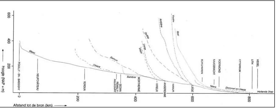
2-1 Gradient of the river Meuse and its tributaries
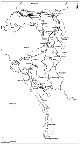
2-2 The catchment of the Meuse
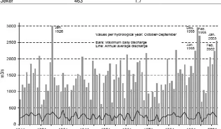
2-3 Discharges on the Meuse at Borgharen
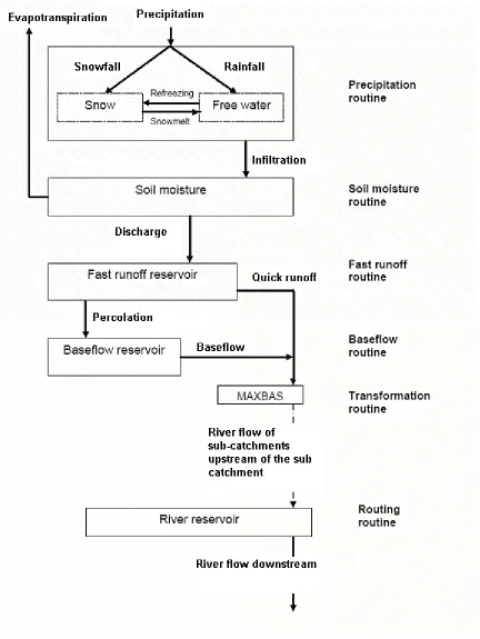
2-4 Schematisation of the HBV-96 model with six routines for one sub-catchment
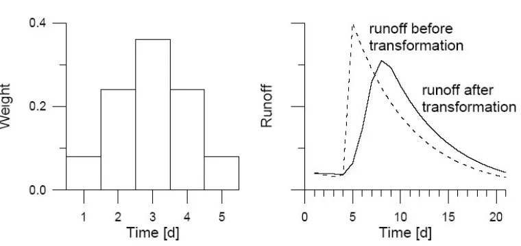
2-5 Example of the transformation function with MAXBAS = 5
2-6 Schematisation of the up stream part of the river Meuse used in the HBV 15 model
3-1 Flow diagram research methodology
3-2 Example of graph with NS Booij and NS model lines and point x
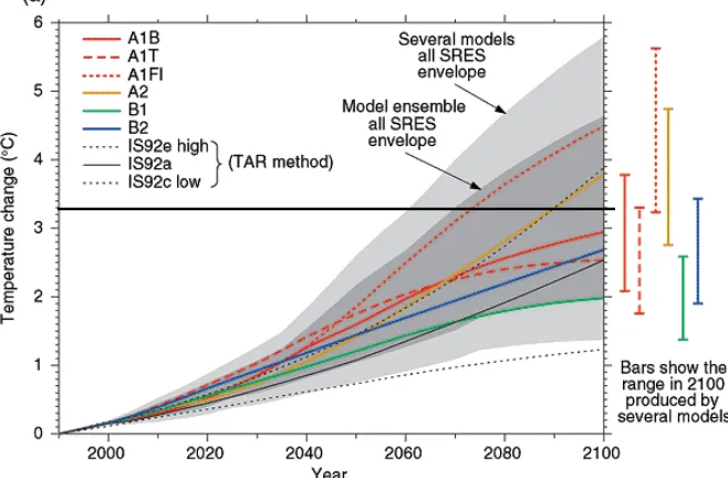
4-1 Temperature change after 1990, six scenarios
5-1 Probability density functions as a result of different uncertainty sources for current climate and changed climate
5-2 NS model and NS Booij values for Vesdre catchment as a function of different related uncertainties in HBV parameters.
5-3 NS model and NS Booij values for Ourthe catchment as a function of different related uncertainties in HBV parameters.
5-4 NS model and NS Booij values for Ambleve catchment as a function of different related uncertainties in HBV parameters.
5-5 NS model and NS Booij values for Lesse catchment as a function of different related uncertainties in HBV parameters.
5-6 Gumbel plot of the peak discharge of the river Meuse
5-7 Annual max discharge with return period of 100 years for current climate and climate change.
List of Tables
2-1 Characteristics (size, gradient, mean discharge, mean annual precipitation) of the differenttributaries.
2-2 HBV parameters.
4-1 Estimations for temperature and precipitation out of Christensen 2004
4-2 The scales and size of the different uncertainty groups
4-3 Mean discharge and NS sub-catchments values.
4-4 Parameters of the sub-catchment of the river Meuse.
5-1 Predictions in temperature and precipitation change and uncertainties
5-2 Modified data sets for Temperature
5-3 Modified data sets for Precipitation
5-4 Model nt Subcatchme
NS for different sub catchments as a function of different related uncertainties in HBV parameters
5-5 Percentages for the uncertainties for all the sub catchments
1
Introduction.
1.1 General
Human society adopts increasingly sophisticated and mechanized lifestyles; consequences are that the amounts of heat-trapping gases in the atmosphere have been increased. By increasing the amount of these gases, humankind has enhanced the warming capability of the natural greenhouse effect. It is the human-induced enhanced greenhouse effect that causes environmental concerns. It has the potential to warm the planet at a rate that has never been experienced in human history. This warming is called climate change. Climate change is more than a warming trend. Increasing temperatures will lead to changes in many aspects of weather, such as wind patterns, the amount and type of precipitation, and the types and frequency of severe weather events that may be expected to occur in an area. Not all regions of the world will be affected equally by climate change. Low-lying and coastal areas face the risks associated with rising sea levels. Increasing temperatures will cause oceans to expand (water expands as it warms), and will melt glaciers and ice cover over land – ultimately increasing the volume of water in the world's oceans (IPCC, 2001a).
Generally, higher temperatures lead to higher potential evaporation and decreased discharge (which also is a function of precipitation, storage, and topography). The storage of water in the soil serves as a buffer; in winter and spring, increasing precipitation normally generates higher discharges because the buffer is full and evaporation is low. During the summer, storage is reduced by evapotranspiration and must be refilled before discharge begins. Seasonal-to-interannual variability in precipitation and temperature also accounts for some of the variability in hydrological characteristics in European river basins. General Circulation Models (GCMs) -based analyses for the European continent (IPCC, 1996) give a range of possible responses of river runoff in a warmer global climate; decreases in some regions (e.g., Hungary, Greece) to increases in other regions (United Kingdom, Finland, Ukraine); these estimates are a function of precipitation, evapotranspiration, and soil moisture projections in the different GCMs. The results of catchment-scale simulations with conventional hydrological models driven by GCM data are highly variable. Arnell and Reynard (1996), for example, simulated changes of ±20% in annual runoff for 21 catchments in Great Britain-with a tendency toward lower amounts of discharge, especially in sensitive areas and during the summer months.
The uncertainties of climate model results, however, remain very large particularly at the regional scale. This limitation is particularly critical for water management practices in the future because water resource impacts occur at the local scale, not at regional or larger scales (Arnell 1999a).
floods occurred in 1993 and 1995 (Wit, 2001). In future with climate change predictions that are more extremer, the discharge of the river Meuse will be higher. But of course there is a lot of uncertainty in the predictions of extreme discharges.
1.2 Problem / previous research
Because of the fact that climate change is a very hot issues for the future of the world many research is performed on this subject. The Intergovernmental Panel on Climate Change (IPCC,2001b) developed emissions scenarios to describe the relationships between the forces driving emissions and their evolution. The scenarios encompass different future developments that might influence greenhouse gas sources and sinks, such as alternative structures of energy systems and land-use. These scenarios are used for climate change prediction all over the world and are the main input in the investigation of climate change and the impact of climate change.
The behaviour of the climate system, its components and their interactions, can be studied and simulated using tools known as climate models. These models are made for studying climate change, weather forecasting and current climate and are called General Circulation Models (GCMs). Arnell (1999b) investigated climate change using different emissions scenarios and global circulation models. He found that global average precipitation will increase. Much of this increase occur over oceans and large parts of land surface. Also the temperature shall rise this will leads to a general reduction in the proportion of precipitation that falls as snow. These changes will have a impact on the discharge of rivers.
The climate change in combination with hydrological models made it possible to investigate the impact of climate change on the hydrological regimes. Dam (1999) investigated the impacts of Climate change and climate variability on hydrological regimes. Middelkoop et. al. (2001) investigated the impact of climate change on hydrological regimes and water resources management in the Rhine basin. He expected that due to climate change the river Rhine will shift from a combined rainfall-snowmelt regime to a more rainfall dominated regime. And that the frequency and height of peak flows will increase. Wit (2001) did research on the effect of climate change on the hydrology of the river Meuse. Out of this research can be concluded that the discharge in spring will increase and that the discharge in summer period will decrease.
Wilby (2005) investigated the uncertainty in water resources model-parameters used for climate change impact assessment. A recommendations out of that research is that climate change impact assessments using conceptual water balance models should routinely undertake sensitivity analyses to quantify uncertainties due to parameter instability, identifiably and non- uniqueness. There are many ways to investigate the HBV uncertainty. Seibert (1997) investigated the uncertainty of a HBV-model performing a Monte Carlo simulation (section 3.2) resulting in a large number of models runs with randomly generated parameters sets. He studied how the measured runoff could be achieved at best with different parameter values. This procedure has the advantage that any interaction between parameters is implicitly taken into account since parameter sets are varied instead of individual parameters. Booij (2005) investigated the impact of climate change on river flooding assessed with different spatial model resolutions. Booij used the HBV model with different sub catchments for the Meuse. He found an increase of 10% in daily average river discharge with an uncertainty in river flooding of 40%. The uncertainties in extreme discharges due to precipitation errors and extrapolation errors are more important than uncertainties due to hydrological model errors and parameters errors.
1.3 Objective and Research questions
The objective of this research is:
To assess the uncertainties in the impacts of climate change on future extreme high discharges of the river Meuse.
The objective has been split up into four research questions;
1). which uncertainties have to be considered in climate change predictions and what is the size of these uncertainties?
2). is there a method to investigate the uncertainty of hydrological models and is it possible to quantify this uncertainty?
3). what is the best way to propagate climatic and hydrological uncertainties through the HBV-15 model with as result the extreme high discharge for the river Meuse with all the uncertainties?
4). what are the most important sources of the uncertainties in the simulated extreme high discharge?
The research performed shall investigate the impact of climate change on the extreme high discharge on the river Meuse but, will also investigate the uncertainty in the extreme high discharge and investigate the size of the uncertainties. The goal is to split up the total uncertainties and quantify the uncertainty groups. The study will focuses on the upstream part of Borgharen on the river Meuse. The extreme discharge on the river Meuse shall be modelled with the HBV-15 model developed by Booij (2005). Not all the uncertainties are considered in this research. Only the uncertainties in the climatological data and the hydrological model are considered.
1.4 Report structure.
2
Meuse catchment: processes and modelling
2.1 Introduction
In this chapter the hydrological model is described. Before that the Meuse catchment is considered in section 2.2. The HBV-model is introduced in section 2.3. In section 2.4 the HBV-15 model that is used in the research is considered and in section 2.5 the calibration of the HBV model is described.
2.2 The Meuse Catchment
2.2.1 General characteristics
The Meuse is a river with a length of 880 km from the source Poulliy-en-Bassigny in France to the mouth the Holandsch Diep in The Netherlands. The Meuse can be divided into 493 km in France, 183 km in Belgium and 204 km in The Netherlands. Its catchment has an area of about 33.000 km2. The Meuse catchment has a temperate climate, with tributaries that are dominated by a rainfall-evaporation regime, which generally produces high flows during winter and low flows during summer. The height of the river above sea level as a function of the distance is shown in figure 2-1. Therefore it can be concluded that the Ourthe, Vesdre, Viroin, Lesse and Amblève have a steep slope and that the Belgian Meuse has a relatively flat slope. The other tributaries are also shown in this figure.
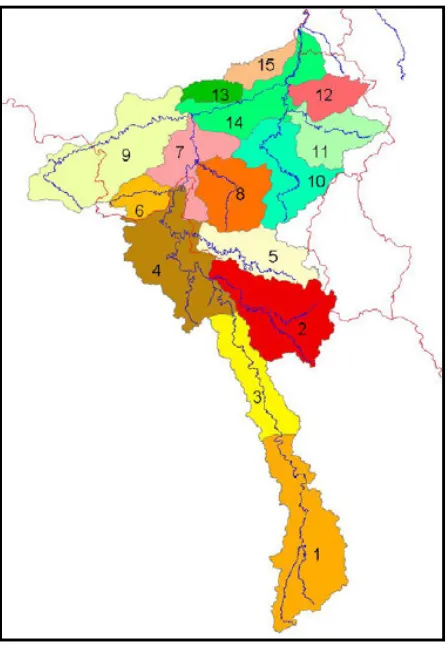
An overview of the catchment of the Meuse is shown in figure 2-2. A good and complete description of the river Meuse and its tributaries is given by Berger (1992).
As far as the hydrologic properties are concerned, the Meuse can roughly be divided into three hydrological zones; the upper reaches, the central reaches and the lower reaches of the Meuse, (Berger, 1992).
The upper reaches (Meuse Lorraine or Lotharingian Meuse), goes from the source at Poulliy-en-Bassigny to the mouth of the Chiers. Here the catchment is lengthy and narrow, the gradient is small and the major bed is wide. The discharge regime is therefore relatively flat.
The central reaches of the Meuse (Meuse Ardennaise or Ardennes Meuse) is situated between the mouth of the Chiers and the Dutch border and transects Palaeozoic rock of the Ardennes Massif. This gives a narrow river valley and a big slope. Together with the poor permeability, this results in a quick response to precipitation. The main tributaries being the Viroin, Semois, Lesse, Sambre and Ourthe.
The lower reaches of the Meuse correspond with the Dutch part of the river. The lower reaches themselves may be split into the stretches from Eijsden to Maasbracht and from Maasbracht to the mouth. In the former part the slope is still relatively large, for this reason it is occasionally reckoned to be part of the Meuse Ardennaise. The stretch that forms the border between Belgium and the Netherlands is called the Grensmaas. Below Maasbracht the river is provided with weirs to make it navigable. The main tributaries are the Roer, Niers and Dieze. In the Roer reservoirs are found, providing a certain minimum discharge. From Boxmeer the river is a typical lowland stream, with summer dikes, flood plains and winter dikes.
2.2.2 Precipitation
The mean annual precipitation in the catchment of the Meuse varies from 800 to 900mm in the south and west to locally 1400mm in the high Ardennes. In particular the total annual rainfall in the catchments of the Semois (1139mm), the Vesdre (1104mm) and the Amblève (1104mm) are high (Berger, 1992), see table 2-1.
2.2.2 Discharges
The variation of the mean discharges over the months is much higher than the variation of the precipitation. This is due to the influence of evaporation, which is highly related to the temperature. As a consequence, discharges in winter are high and discharges in summer are low. Almost all floods in the Meuse catchment have been observed during the winter season. One exception is the flood of July 1980 with a peak discharge of about 2000 m3/s measured at Borgharen, see figure 2-3.
A flood arises when in a short period of time, approximately ten days; the amount of precipitation in the catchment is high. The highest known discharge ever measured at Borgharen was 3000 m3/s during the floods of 1926 and 1993.
Tributary Size Gradient Mean discharge Mean annual Precipitation (Km2) (x 10-4) (m3/s) (mm)
Meuse source- St.Mihiel 2540 26.3
Chiers 2222 10 27 859
Meuse St. Mihiel-Stenay 1364 20
Meuse Stenay- Chooz
Semois 1358 15 27 1139
Viroin 593 20 6.9 940
Meuse Chooz-Namur
Lesse 1314 50 16 954
Sambre 2863 7 28 825
Ourthe 5223 37 23 968
Vesdre 677 80 9.4 1104
Ambleve 1052 50 19 1104
Mehaigne 345 2.3
Meuse Namur- Borgharen
Jeker 463 1.7
The Meuse fulfils many functions, which are subject to droughts as well as to floods. These are: drinking water production, agriculture, recreation, water supply industry, inland navigation, nature, safety and cooling water.
Table 2-1 characteristics (size, gradient, mean discharge and mean annual precipitation) of the different tributaries. (Berger, 1992).
2.3 HBV model
2.3.1 Introduction
Out of previous research is found that the HBV model is very appropriate for flood frequency analysis. Especially for assessments of climate change impacts on peak discharges (Booij, 2002). This and the fact that the model could be easily obtained, is the reason for using the HBV model in this research.
2.3.2 Background
The HBV model (Bergström and Forsman, 1976; Bergström et al., 1992) is a rainfall-runoff model, which includes conceptual descriptions of hydrological processes at the catchment scale (conceptual hydrological model). The HBV model has been developed by the Swedish Meteorological and Hydrological Institute (SMHI) in Norrköping, Sweden, by Bergström. The HBV-model is named after the abbreviation of Hydrologiska Byråns
Vattenbalansavdelning (Hydrological Bureau Water balance-section). This was the former section at SMHI where the model was originally developed. Different versions of the HBV model have been applied in more than 50 countries all over the world. It has been applied to countries with such different climatic conditions as for example Sweden, Zimbabwe, India and Colombia. HBV can be used as a semi-distributed model by dividing the catchment into sub catchments.
Input data are observations of precipitation, air temperature and estimates of potential evapotranspiration. The time step is usually one day, but it is possible to use shorter time steps. The evaporation values used are normally monthly averages although it is possible to use daily values. Air temperature data are used for calculations of snow accumulation and melt. It can also be used to adjust potential evapotranspiration when the temperature deviates from normal values, or to calculate potential evaporation. If none of these last options are used, temperature can be omitted in snow free areas. The model consists precipitation routine, soil moisture routine, quick runoff routine, baseflow routine, transformation routine and a routing routine It is possible to run the model separately for several sub catchments and then add the contributions from all sub catchments (Bergström, 1995) see section 2.3.2.
2.3.3 Structure HBV-model
A schematic sketch of the structure of the HBV-96 model is shown in figure 2-4. As can be seen from this figure the models consists the following six model routines:
• Precipitation routine • Soil moisture routine • Quick runoff routine • Baseflow routine
• Transformation function • Routing routine.
Each one of the sub-catchments has individual soil moisture accounting procedures and response functions. Therefore, the runoff is generated independently from each one of the sub catchments. The six model routines and their interactions that are illustrated in figure 2-4 for one sub catchment and are described below based on (Booij, 2002) and (Deckers, 2006).
Precipitation routine
Precipitation can occur as rainfall or snowfall. Snowfall occurs if the air temperature T [C0] is below a defined temperature TT [Co] and rainfall occurs if T >TT. Snowfall is added to the dry snow reservoir (within the snow pack) and rainfall is added to the free water reservoir, which represents the liquid water content of the snow pack. Interactions between these two components take place through snowmelt and refreezing, respectively shown in equation [2-1] and [2-2]:
(
T TT)
CFMAX
PSNOW = × − [2-1]
(
TT T)
CFMAX CFR
PRAIN = × × − [2-2]
CFMAX = melting factor [mm/ (d C0)] CFR = refreezing factor [-]
Soil moisture routine
The soil moisture routine is the main part controlling runoff formation. Three output components are generated in this routine: direct runoff, indirect runoff and actual evapotranspiration
Direct runoff
moisture reservoir. Otherwise the precipitation becomes directly available for runoff (DR,
[mm/d]) as shown in equation [2-3]:
(
)
{
SM
P
FC
,
0
}
MAX
DR
=
+
−
SM =FC DR=P [2-3]From equation [2-3] the volume of infiltrating water into the soil moisture reservoir (IN,
[mm/d]) equation [2-4] is:
DR P
IN = − [2-4]
A part of this infiltrating water will contribute to the soil moisture content SM; the other part will run through the soil layer as indirect discharge R.
Indirect runoff
The indirect discharge (R, [mm/d]) through the soil layer is determined by the amount of infiltrated water (IN) and the soil moisture content (SM, [mm]), through a power relationship with parameter . This is shown in equation [2-5]:
β
=
FC SM IN
R [2-5]
From this relation follows that the indirect discharge is increasing with increasing soil moisture content. For a smaller value of , the increase is stronger. In equation [2-5] it is also assumed that as long as there is no infiltration, there is no indirect runoff. The amount of water that does not run off is added to the soil moisture.
Evapotranspiration
Actual evapotranspiration (EA, [mm/d]) which occurs from the soil moisture routine is
related to the measured potential evapotranspiration (EP [mm/d]), soil moisture state and
a parameter value LP, [-]. LP is a fraction between 0 and 1 and denotes the limit where above the evapotranspiration reaches its potential value. This relation is shown in equations [2-6] and [2-7]:
P
A LP E
SM
E = × With
SM
<
(
LP
×
FC
)
[2-6]P A
E
E
=
WithSM
≥
(
LP
×
FC
)
[2-7]Quick runoff Routine
The runoff routine is the response function which transforms excess water from the soil moisture routine to runoff. In this transformation three processes can be distinguished which are; percolation to the base low, capillary transport from quick runoff reservoir back to the soil moisture routine and quick runoff.
Percolation
The outflow of the soil moisture routine, DR+ R, is available for the fast and base flow routine. The direct runoff (DR) and indirect runoff (R) together enter the quick runoff reservoir from which a specific amount percolates through to the underlying baseflow runoff reservoir. Percolation (PERC, [mm/d]) only occurs when there is indirect and or direct runoff
Capillary rise
The second process in this routine is the capillary upward transport to the soil moisture reservoir from the quick runoff reservoir. The capillary flow [mm/d] depends on the amount of water stored in the soil moisture zone. The parameter CFLUX [mm/d], a maximum value of capillary flow, limits the capillary flow. The capillary flow depends on the soil moisture deficit, FC- SM. When there is no soil moisture deficit, no capillary rise will occur. Otherwise, a fraction of CFLUX will flow capillary upward. This is shown in equation [2-8]
− ×
=
FC SM FC CFLUX
Cf [2-8]
Quick runoff
When the yield from the soil moisture routine is higher than PERC and Cf allows and water is available in the quick runoff reservoir, quick runoff (Q0, [mm/d]) is determined
through equation [2-9]
(+α)
×
=
10
K
UZ
Q
f [2-9]Figure 2-5. Example of the transformation function with MAXBAS =5 (Seibert, 2002)
Baseflow routine
The baseflow Q1[mm/d] out of the Baseflow reservoir is the second part of the response
function. The reservoir represents the groundwater contribution of the catchment.
The recession coefficient Ks [d-1] is the only calibration parameter of this linear reservoir.
The baseflow is represented by equation [2-10]:
LZ K
Q1 = S × [2-10]
In which LZ is the water level in the reservoir [mm].
Transformation routine
Routing routine
With the transformation function, per sub catchment discharge runoff will be generated. In the routing routine HBV links the sub catchments to each other by adding the runoff from accompanying sub catchments to the local runoff. The inflow from another sub catchment is assumed to flow through a river channel from the outlet of the upstream catchment to the outlet of the current catchment where the local runoff is added. Besides plain linkage of the sub catchments, it is possible to delay the water in the river channel by using the parameters LAG and DAMP. A modified version of the Muskingum equation is used for this computation. This is shown in equation [2-11]. In brief, this equation simulates the attenuation of the wave amplitude (the parameter DAMP) and the passage time (the parameters LAG) of the discharge through the sub catchment.
By the parameters LAG, the river channel will be subdivided into a number of segments. When this parameter is an integer, each segment will refer to a delay of one day. If DAMP has a value of zero, the outflow from a segment equals the inflow to the same segment during the preceding time step, so that the shape of the hydrograph is not changed. If DAMP is not zero the shape will be changed, as the outflow from a segment will depend on the inflow during the same time step as well as the inflow and outflow at the preceding step. This is shown in equation [2-11]
( )1 1 ; 1 ;( )1 2
;
; Q C Q C Q C
QOUTt = OUT t− × + INt× + IN t− × [2-11]
Where t is the current step and t -1 the previous time step. The coefficients C1 and C2 are defined through equations [2-12] and [2-13];
(
DAMP)
DAMP C
+ =
1
1 [2-12]
(
)
(
DAMP)
DAMP C
+ − =
1 1
2.4 HBV-15 Model.
Booij (2002) developed a HBV model especially for the Meuse catchment and used is used in this study. This model called the HBV-15 model uses 15 sub-catchments upstream of Borgharen. The schematisation is shown in Figure 2-6. The model does not include locks, weirs, reservoirs or other man made structures. Calibration and validation of the model is performed for the whole catchment but also for the sub-catchments Vesdre, Amblève, Lesse and Ourthe. In section 3.4 the calibration results shall be used for the uncertainty analysis of the model parameters.
The HBV-15 model is available in an user interface from (SMHI) as well as in a FORTRAN code. In the user interface setting, simple standard simulation can be made. The model will simulate discharges that are the results of one run of the model. The FORTRAN model is especially useable for simulations with multiple runs. Furthermore it is easy to modify the model and make slight changes to the model setting. Therefore the FORTAN model shall be used to make the simulations runs in this research.
Figure 2-6 Schematisation of the upstream part of the river Meuse, used in the HBV-15 Model. Legend;
2.5 Calibration
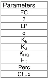
A sensitivity analysis has been performed to asses the influence of individual or multiple parameters on the output of the model. This can be used to determine the parameter set that generates optimal model results. The six key parameters are FC, LP, , , KS and Kh. This 6 different parameters shall be used in the research the others parameters out the HBV-model will stay constant. (All parameters are shown in table 2-2) This is because these parameters are not important to find the uncertainty of the HBV-model. In order to define the values of the 6 important parameters used in the HBV-model, these parameters are calibrated against observed discharge whereby the model parameters are adjusted until the observed natural system output showed an acceptable level of agreement (Booij, 2005). The calibration of the HBV-model has been performed by Booij (2005)
The optimality of the model output (discharge) has been assessed in different ways, namely by applying the Nash-Sutcliffe efficiency coefficient R2 (Nash- Sutcliffe, 1970), the relative volume error RVE and the relative extreme value error REVE. They are outlined below presented by equations [2-14], [2-15] and [2-16]
• Nash-Sutcliffe coefficient, R2
(
)
(
)
2, 1 2 , , 1 2 1 obs i obs n i i obs i sim n i Q Q Q Q R − − − = − = [2-14]
• Relative volume error, RVE
%
100
, 1 1 , , 1×
−
=
− = = i obs n i n i obsi i sim n i EQ
Q
Q
RV
[2-15]Relative extreme value error REVE
( )
( )
( )
T
RV
T
RV
T
RV
REVE
obs obs sim−
×
=
100
[2-16]Where i is the time step, n is the total number of time steps, Q is the discharge. Subscripts obs and sim means observed and simulated and RV (T) is the t-year return value.
parameter value can be studied by testing the sensitivity of the model by calculating the Nash-Sutcliffe efficiency coefficient R2 (Nash-Sutcliffe, 1970) see equation [2-14].
It compares the modelled discharge values (Qsim, i) with the measured discharge values (Qobs, i) and measured average value (Qobs,i ). The range of the Nash-Sutcliffe value is
from - to 1. Hydrologic models are considered to be good when the coefficient is 0.8 or higher, (Booij 2005).
Table 2-2 HBV parameters.
Parameters
FC
LP
Kh
KS
KHQ
HQ
• HBV model
• Monte Carlo Simulations
• Stat. frey analyse
• HBV model
• Monte Carlo Simulations
• Stat. frey analyse
3
Methodology
3.1 Introduction
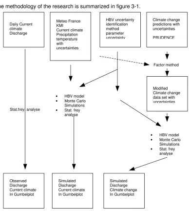
The methodology of the research is summarized in figure 3-1.
Figure 3-1 Flow diagram research methodology
The basis for this research are two studies performed by PRUDENCE. The results of these studies are climate change predictions for temperature and precipitation and uncertainties herein. These climate change data is transformed to the Meuse catchment with a climate change factor and the current climate for the Meuse catchment. The new climate data are presented in a normal distribution. The uncertainty in the data is expressed in the standard deviation. The different uncertainty sources are propagated through the HBV model using Monte Carlo simulations. Before the HBV-model is run, a
Daily Current climate Discharge
Meteo France KMI
Current climate Precipitation temperature with uncertainties
Climate change predictions with uncertainties
PRUDENCE HBV uncertainty
identification method parameter uncertainty
Simulated Discharge Current climate In Gumbelplot
Factor method
Observed Discharge Current climate In Gumbelplot
Simulated Discharge Climate change In Gumbelplot
special uncertainty analysis for the HBV-15 model is preformed. The output of the model is the extreme discharge of the river Meuse. In section 3.2 the Monte Carlo simulation is considered. The method for preparing the climate data is considered in section 3.3. The investigation of the uncertainty of the HBV-15 Meuse model is described in section 3.4. Finally in 3.5 the extreme discharge is considered.
3.2 Monte Carlo Simulation
The main aim of this research is to find the uncertainty in the extreme discharge on the Meuse. The discharge shall be simulated with the help of the HBV-15 model. That is why it is important to know how the different uncertainties develop during running the HBV -15 model and how to quantify them in the output. There is chosen to propagate the modified climate data for the Meuse with all uncertainties through the model with a Monte Carlo analysis. There is chosen for a Monte Carlo analysis because it has been used in previous researches for the same kind of problems, (Booij, 2005).
In a Monte Carlo analysis, a value is drawn randomly from the distribution for each input. Together this set of random values, one for each input, defines a scenario, which is used as input to the model, computing the corresponding output value. The entire process is repeated n times producing n independent scenarios with corresponding output values. These n output values institute a random sample from the probability distribution over the output indicated by the probability distribution over the inputs, (Morgan and Henrion, 1990).
There shall be made 1000 runs in one Monte Carlo simulation. This amount of runs is bases on the fact that less runs will make the predictions not certain enough. More runs will take a lot more process time and the predictions are not more certain. So therefore there is chosen to do 1000 runs in a simulation. The model shall be run with different uncertainty groups. This way it becomes possible to investigate what the propagation of the different uncertainty groups through the HBV-15 model are and what the sizes of the uncertainty groups are according to the extreme discharge.
The uniform distribution is the simplest continuous statistical distribution in probability. It has a constant probability density on an interval (a, b) and zero probability density elsewhere. The continuous uniform distribution is a generalization of the rectangle function because of the shape of its probability density function. It is parameterized by the smallest and largest values that the uniformly-distributed random variable can take, a and b, (Morgan and Henrion, 1990). In this research the different parameters of the HBV-15 model are assumed to be distributed in an uniform distribution. This is assumed because of the fact that is it not for sure that kind of distribution the parameters will have so there for it is assumed that it will be a uniform distribution because it is the simplest. The uniform distribution is necessary for the investigation of the uncertainty of the HBV-model. See section 3.4.
is in a normal distribution. (Déqué, 2004; Christensen, 2004) And the fact that it is a nature phenomenon. So through the normal distribution it was possible to use the climatological data as input for the HBV-15 model. This is because of the fact that during performing a Monte Carlo analyse the values are randomly chosen and the probability is the chance on a certain value. This chance is used to calculate the uncertainty in the data output of the HBV-model. See section 3.3.
3.3 Uncertainties in climate change variables
3.3.1 Predictions of temperature and precipitation
The basis for the research are two different studies performed within the framework of the EU-project PRUDENCE. PRUDENCE is a project funded by the European Commission under its fifth framework programme. It has 21 participating institutions from a total of 9 European countries, with several additional international collaborators, which have contributed to the project from their own funding. The PRUDENCE project is devoted to the study of climate changes over Europe. It has two main objectives: to estimate the uncertainties about the expected response, and to evaluate possible impacts in various fields of human activities (PRUDENCE, 2006).
The first study is performed by Christensen (Christensen, 2004). Christensen did research on the prediction of climate change for different countries in Europe. The analysis is based on all PRUDENCE simulations with RCMs and on a country-by-country basis. For each country-by-country (some of the larger countries are split in two sections) all available simulation data for temperature and precipitation have been aggregated into one number per field representing this country for each simulation. This number is scaled according to the global temperature change using the underlying global climate model, which has been used as a driver for the regional climate model. This way, more than 25 estimates of the change in temperature and precipitation has been provided for countries in Europe (Christensen, 2004).
The estimations for temperature and precipitation are given for the seasons: December, January and February (DJF), March, April and May (MAM), June, July and Augusts
(JJA) and September, October and November (SON). And are the averages of the
whole country. The estimations for temperature are expressed as: TCH, SEASON, [Co] and
the estimations for precipitation are expressed as: PCH, SEASON, [%].
The change in precipitation and temperature for a country expressed as: PCHANGE, SEASON,
[%] and temperature expressed as: TCHANGE, SEASON, [Co] can be predicted when the
estimations PCH, SEASON and TCH, SEASON are multiplied with the global average temperature
change expressed as: TGA, [Co] as shown in equation [3-1] and [3-2]:
GA SEASON CH SEASON
CHANGE P T
P , = , × [3-1]
GA SEASON CH SEASON
CHANGE P T
T , = , × [3-2]
model uncertainties (Christensen, 2004). Because of the fact that the predictions given by Christensen are independent of specific choices of emission scenario, the uncertainties of the different emission scenarios are not present in the estimates of the projected changes.
Christensen gives an uncertainty range of the predictions of temperature and precipitation change which is expected to be the standard deviation expressed as PCH, SEASON, [%] for the precipitation and TCH, SEASON, [C0] for the temperature.
The total uncertainty in precipitation and temperature for a country expressed as:
PCHANGE, SEASON, [%] and temperature expressed as: TCHANGE, SEASON, [Co] can be
estimated in the same way as the total change is estimated. Thus the estimations PCH, SEASON and TCH, SEASON are multiplied with TGA as shown in equation [3-3] and [3-4]:
GA SEASON CH SEASON
CHANGE P T
P , =
σ
, ×σ
[3-3]GA SEASON CH SEASON
CHANGE P T
T , =
σ
, ×σ
[3-4]The sizes of the different uncertainty groups are not investigated by Christensen, but have been studied by Déqué (2004). Déqué investigated the uncertainty in the results of ten regional climate models (RCMs).
The objective of the study performed by Déqué is to focus on the response of a few General Circulation Models used in the PRUDENCE project. Déqué has restricted to 30-year seasonal means. Moreover, amongst the many fields archived in the PRUDENCE database, Déqué selected temperature and precipitation. These fields offer the triple advantage to be directly connected to human perception of the climate, to be comparable with reliable observations, and to exhibit regional-scale features that are not accessible to coarse resolution GCMs. In order to further reduce the size of his report, Déqué concentrated on the two extreme seasons winter (DJF) and summer (JJA).
Déqué used the ten RCMs available in the PRUDENCE seasonal database. The models are those of CNRM, DMI, ETHZ, GKSS, Hadley Centre, ICTP, KNMI, MPI, SMHI and UCM. Out of the ten RCMs, three models (CNRM, DMI and Hadley Centre) have produced three 30-year simulations. For the other seven, Déqué have triplicated the single simulation in order to give the same weight to each model. For the prediction of Europe two emission scenarios are used namely the A2 and B2 scenarios of the SRES emission scenarios of the IPCC.
same models as the GCMs but now special build for smaller areas. The uncertainties are given for the season DJF and JJA for temperature as well for precipitation.
There is a problem because of the fact that there are used two different researches. But Christensen and Déqué used the same data sources namely PRUDENCE. Therefore it is possible to combine the result of both researches by only transforming the results of the research of Déqué to the results of Christensen. So it becomes possible to use the sizes for the different uncertainty groups found by Déqué (2004), to split up the total uncertainty found by Christensen (2004).
In the transforming process the sizes of the different uncertainties groups, are made usable for splitting up the total uncertainty in the predictions for temperature and precipitation ( TCHANGE, SEASON and PCHANGE, SEASON). The sizes of different uncertainty
groups TSDn, SEASON, [Co] and PSDn, SEASON, [%] are necessary to investigate the
contribution of one uncertainty group to the extreme discharge. The transformation process is shown in equations [3-5] and [3-6]:
× Σ
= n
SEASON CHANGE
n SEASON SEASON
SDn T SD
SD T
,
,
σ
σ
[3-5]× Σ
= n
SEASON CHANGE
n SEASON SEASON
SDn P SD
SD P
,
,
σ
σ
[3-6]The temperature uncertainty for one uncertainty group n can be calculated, when the sum of the four different uncertainties group divide by the total uncertainty out of Christensen(2004) is multiplied with the size of the group n. The size of the different groups is come out of Déqué (2004). This is the same for precipitation but that with the uncertainty for the precipitation.
3.3.2 Modified data set
When the change in precipitation and temperature for a country (PCHANGE, SEASON and
TCHANGE, SEASON) is calculated with equations [3-1] and [3-2] and the sizes of the different
uncertainty groups are calculated with equations [3-3] to [3-6], it becomes possible to calculate the modified data set. For this step a so called climate factor method (CF) is used. This CF is the same as used in Diaz-Nieto and Wilby, (2005). The CF method calculates climate series by adding (temperature) or multiplying (precipitation) with the observed series. The change in precipitation and temperature is transformed to the modified data expressed in PNEW, SEASON [mm] and TNEW, SEASON [Co] with the help of the
observed data expressed in TCURRENT [Co] and PCURRENT [mm] shown in equations [3-7]
and [3-8]:
CURRENT SEASON
CHANGE SEASON
NEW T T
T , = , + [3-7]
CURRENT SEASON
CHANGE SEASON
NEW P P
P , = , × [3-8]
In the study performed by Déqué only two different emissions scenarios are used. So uncertainty for the different scenarios is not well investigated in the studies performed by Déqué (2004) and Christensen (2004). Therefore it is necessary to have a better look at the uncertainty for emission scenarios. To find the uncertainty for the emission scenarios figure 4-1 (section 4.2) from the IPCC shall be used.
3.4 Method to estimate parameter uncertainties.
The reliability of hydrological conceptual models is highly depending on the calibration procedure, which is the search for an optimal parameter set. See section 2.5
The method is bases on the next the assumptions:
1. The uncertainty of a model can be expressed in a Nash Sutcliff coefficient, which is compareness between the observed and simulated discharge.
2. The uncertainty of a model can be simulated trough parameters variation.
3. Through the variation of the parameters without correlation between them, different model world can be created. The range where in the parameters are verified is chosen shuts a way that de average NS coefficient out of the comparers of the different model world is equal to the ns coefficient mentioned at point 1.
It is also assumed that the uncertainty of the parameters expressed in the form of a standard deviation is the major source of the uncertainty of the model outcome. Through consideration of this parametric uncertainty, model structural and scale related uncertainties are not taken into account. However, these are assumed to be at least partly covered by the parametric uncertainty.
In previous research (e.g. Booij, 2002; Arends, 2005) the calibration and investigation of parameters for the HBV-15 models has been performed. The most important parameters are FC, LP and Beta in the soil moisture routine and Alpha, Kf and Ks in the fast flow routine, (Booij, 2002). This 6 different parameters shall be used in the research the others parameters out the HBV-model will stay constants. This is because this parameters are not important to find the uncertainty of the HBV-model. A Monte Carlo model simulation with these parameters values creates a Nash-Sutcliffe efficiency coefficient R2 for the total Meuse catchment (NS
Meuse) for the calibration and the
validation period of total 27 years (Booij, 2002). (See section 2.5) There are also Nash-Sutcliffe values for four sub catchments namely: Vesdre (NSVesdre), Ourthe (NSOurthe),
Ambleve (NSAmbleve) and the Lesse (NSLesse). The values of the main parameters and the Nash-Sutcliffe coefficients shall be used in this research for the uncertainty analysis of the HBV model.
To find the standard deviation ( parameters, sub-catchment) for the parameters there shall be
calculated a certain percentage of the mean value of the parameters. This percentage ( ) will create a certain range (- ;+ ) around the mean value of the parameter. This range could be considered as an uncertainty belt. So with a certain percentage of the mean value of a parameter a standard deviation for that parameter is created.
0.6 0.65 0.7 0.75 0.8 0.85 0.9 0.95 1
5 10 15 20 25 30 35
(%) N as h-S ut cl iff e co ef fic ie nt NS model NS Booij
discharge series are compared with each other instead of observed discharges. See equation [3-9].
(
)
(
)
21 2 1 1 m m n i m n n i Matrix Q Q Q Q NS − − − = − = [3-9]
Q= Extreme discharge Series n = 1 to 1000
m= 1 to 1000 n m
When all the discharge series are compared with each other a matrix can be made of all the NSmatrix values. The matrix has the scale of n x n. So there are n2 NSmatrix values in one matrix. The average Nash Sutcliffe value of the matrix expressed in Model
nt Subcatchme
NS can
be calculated with equation [3-10]. The diagonal out of the matrix is not used in the calculation of the average, this is because the diagonal are the results of the compares of the same discharges and the results are 1,0. When these values are also used for calculating the average, the value for the average will be to high.
(
1000 1000)
/
1000 2 −
− = m+n
Model nt
Subcatchme NS
NS [3-10]
The Model nt Subcatchme
NS value can be printed in a graph. When this process is performed for different percentages it is possible to draw a graph of the Model
nt Subcatchme
NS values as a
function of the different percentage for specific sub- catchment.
When the NSsub-catchment, value out of Booij 2002, is also printed as a horizontal line in the
graph it becomes possible to read of the percentage at which the Model nt Subcatchme
NS is equal to
NSsub-catchment. See figure 3-2 as an example.
The percentages expressed as p [%] (where the two values are equal) is taken to calculate the range and so the standard deviation of the parameters that are used for those sub-catchments. This process is performed for the sub-catchments the Lesse, Ambleve, Ourthe and the Vesdre. For the other 11 sub-catchments an average of the four catchments has been calculated. In the calculation of the average, the size of the discharge of the different sub catchments is used as weight. The found Pcatchment value
for each sub-catchment is used to calculate the uncertainty range for the parameters of that sub-catchment. This range with the mean value shall be put into the model as the parameter uncertainty. A control Monte Carlo simulation shall be performed. With the results of this simulation a Nash-Sutcliffe coefficient (NSmodel) shall be calculated. This
value will be compared with the calibrated Nash-Sutcliffe coefficient for the Meuse catchment (NSMeuse.) (This is the Nash Sutcliffe coefficient at Borgharen, calculated with
equation [2-17]. When both values are almost equal the method of analysing the uncertainty of the HBV model is performed quite well. The HBV uncertainty expresses in the parameters shall be split up into the main routing processes of the HBV model. These routings are the soil moister, the quick runoff and the base flow.
3.5 Gumbel distribution, extreme discharge
In probability theory and statistics the Gumbel distribution (named after Emil Julius Gumbel (1891–1966)) is used to find the maximum of a number of samples of various distributions. For example it can be used to find the maximum level of a river in a particular year if we have the list of maximum values for the past ten years. It is therefore useful in predicting the chance that an extreme earthquake, flood or other natural disaster will occur. The Gumbel distribution, and similar distributions, are used in extreme value theory and is also known as the log-Weibull distribution, (Morgan and Henrion, 1990). In this research the Gumbel distribution is used for calculating the extreme discharge of the river Meuse.
To calculate the extreme high discharge with a certain return period and to make a figure with a Gumbel distribution of the extreme high discharge the equation 3-11 and 3-12 are used, (Shaw, 1994).
−
+
Π
−
=
1
)
(
)
(
ln
ln
6
)
(
X
T
x
T
T
K
γ
K(T) is the frequency factor. [3-11]Thus if an estimate of the annual maximum discharge with a return period of 100 years is required, then T(X) = 100 years, K(T) = 3.14, = 0,55772
The estimation of the extreme discharge expressed in Qextreme with a specific return period is shown in equation [3-12]:
σ
×
+
=
Q
K
(
T
)
Q
extreme [3-12]4
Data
4.1 Introduction
In chapter 3 the methodology of the research has been considered. In this chapter all the necessary data and other values needed for performing the research according to the methodology are treated. In section 4.2 the findings out of the report of Christensen are described for the Meuse catchment and the global warming out of the report of the IPCC is described. The main points out of the report of Déqué, the different sizes for the uncertainty groups and the uncertainty for the emission scenarios are considered in section 4.3. Finally, in section 4.4 the HBV-15 calibration data needed for the calibration of the model and for performing the uncertainty analysis method are considered.
4.2 Change of current climate
The research area is the river basin upstream of Borgharen. The main countries in this area are Belgium, Luxemburg en France. The estimations for temperature and precipitation of Christensen (2004) are used. These are land average values. Because of the fact that France is a very large country with different climates, the data for France are not considered in this research. The data for Belgium and Luxemburg are considered for calculating the average that shall be used in the research
For each variable the results are shown as follows:
TCH,SEASON : Estimate of the mean values from all models TCH, DJF : Estimate of standard deviation from all models
Temperature T CH,DJF T CH,MAM T CH JJA T CH,SON TCH, DJF TCH,MAM TCH, JJA TCH,SON
Belgium 1.0 1.0 1.5 1.3 0.3 0.4 0.5 0.3 Luxemburg 1.0 1.0 1.6 1.3 0.3 0.4 0.5 0.4 Averge 1.0 1.0 1.55 1.3 0.3 0.4 0.5 0.35
Precipitation
% P CH,DJF P CH,MAM P CH JJA P CH,SON PCH, DJF PCH,MAM PCH, JJA PCH,SON
Belgium 6.5 0.0 -11.0 -2.3 3.1 2.6 4.4 3.0 Luxemburg 7.8 -0.2 -9.9 -2.0 2.7 2.8 3.7 3.1 Average 7.15 -0.1 -10.45 -2.15 2.9 2.7 4.05 3.05
Table 4-1 shows the data from Christensen (2004). The data are given seasonally DJF (Dec. – Jan. – Feb.), MAM (Mar. – Apr. – May), JJA (Jun. - Jul. – Aug.) and SON (Sep. – Oct. – Nov). The upper part gives the estimations for the temperature per 1 °C global warming for Belgium and Luxemburg. The lower part projects the estimations of relative change in precipitation for a 1°C global warming for Belgium and Luxemburg. The uncertainty in the estimations as expressed in the standard deviation of the mean values. Due to the fact that the changes and the uncertainties are expressed relative to a 1 °C global warming, the change in precipitation and temperature for a country can be predicted when the given changes are multiplied with the global average temperature change expressed as: TGA [Co] (see section 3.3).
The change in precipitation and temperature for the countries Belgium and Luxemburg can be found when the given changes are multiplied with the global average temperature change expressed in: TGA, [Co]. According to the IPCC, 2001a the average global warming for the year 2100 is about 3.3 °C (see figure 4-1 the dark gray section the mean value) (indicated by the straight black line). So the estimations from Christensen (2004) have to be multiplied with 3.3 to get the predictions expressed in:
PCHANGE, SEASON, [%] and TCHANGE, SEASON, [Co] for the year 2100.
4.3 Uncertainties in the climate change
In the predictions of Christensen (2004) is not given a distribution of the different uncertainty groups. Only a total uncertainty expressed as the standard deviation and mean values for temperature and precipitation change. Therefore the results of the study preformed by Déqué (2004) shall be used to get the size of the different uncertainty groups that must be considered in the climate change predictions.
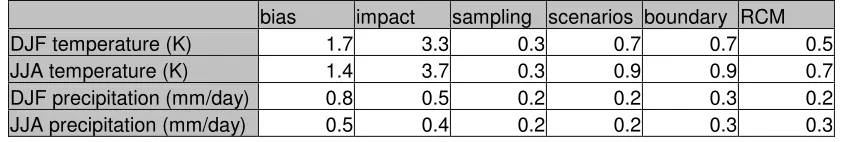
In table 4-2 the size of the different uncertainties according to total uncertainty and climate impact are shown. The standard deviations due to sampling (SD1), emission scenarios (SD2), GCMs (SD3) and RCMs (SD4) are given. These sizes shall be used to split the total uncertainties in the predictions for temperature and precipitation ( TCHANGE, SEASON and PCHANGE, SEASON) into different uncertainty-groups. This way it becomes
possible to create climate data with uncertainties expressed in different standard deviations for each uncertainty group expressed in TSDn, SEASON, [Co] and PSDn, SEASON,
[%].
Déqué did only inv