An approach to performance assessment and fault diagnosis for rotating machinery equipment

An approach to performance assessment and

fault diagnosis for rotating machinery equipment

Xiaochuang Tao

, Chen Lu

, Chuan Lu

and Zili Wang

Abstract

Predict and prevent maintenance is routinely carried out. However, how to address the problem of performance assessment maximizing the use of available monitoring data, and how to build a framework that integrates performance assessment, fault detection, and diagnosis are still a significant challenge. For this purpose, this article introduces an approach to performance assessment and fault diagnosis for rotating machinery, including wavelet packet decomposition for extracting energy feature samples from vibration signals acquired during normal and faulty conditions; clustering analysis for demonstrating the separability of the samples; and Fisher discriminant analysis for providing an optimal lower-dimensional representation, in terms of maximizing the separability among different populations, by projecting the samples into a new space. In the new low-dimensional space, the

Mahalanobis distance (MD) between the new measurement data and normal population can be calculated for performance assessment. Moreover, this model for performance assessment only requires data to be available in normal conditions and any one of all possible fault conditions, without the necessity for the full life cycle of condition monitoring data. In addition, if monitoring data under different fault conditions are available, the fault mode can be identified accurately by comparing the MDs between the new measurement data and each fault population. Finally, the proposed method was verified to be successful on performance assessment and fault diagnosis via a hydraulic pump test and a ball bearing test.

Keywords:Performance assessment, Fault diagnosis, Fisher discriminant analysis, Mahalanobis distance

1. Introduction

Currently, driven by the demand to reduce maintenance costs, shorten repair time, and maintain high availability of equipment, maintenance strategies have progressed from breakdown maintenance (fail and fix) to preventive main-tenance, then to condition-based maintenance (CBM), and lately toward a prospect of intelligent predictive mainte-nance (predict and prevent), [1-3]. While the reactively breakdown maintenance and blindly preventive mainte-nance do sometimes reduce equipment failures, they are more labor intensive, do not eliminate catastrophic failures and cause unnecessary maintenance. This is where CBM steps in. It was reported that 99% of mechanical failures especially rotating machinery are preceded by noticeable indicators [4]. That is to say, with the exception of abrupt,

catastrophic failures, most faults of rotating machinery equipment have progression processes to failure. We can view the deterioration as a two-stage process: the first stage as normal operation, and the second stage as a potential failure [5,6]. Of interest here is when the second stage starts and how it develops. CBM attempts to monitor ma-chinery health based on condition measurements that do not interrupt normal machine operation. Rotating machi-nery is one of the most common classes of machines. Over the past few years, technologies in condition monitoring, fault diagnostics, and prognosis for rotating machinery, which are important aspects in a CBM program, have been receiving more attention. Because fault diagnosis problems can be considered as classification problems [7], Fisher dis-criminant analysis (FDA), which is studied in detail in the pattern classification literature, has been applied to con-duct fault diagnosis. However, at present, its application has mainly been concentrated to industrial process (espe-cially chemical processes), but rarely to rotating machinery * Correspondence:luchen@buaa.edu.cn

1_{School of Reliability and Systems Engineering, Beihang University, Beijing} 100191, People’s Republic of China

2_{Science & Technology Laboratory on Reliability & Environmental} Engineering, Beijing 100191, People’s Republic of China

equipment [8-11]. Moreover, although performance assess-ment, fault detection, diagnosis, and prognosis have received increased attention with significant progress [12], currently, few methods can realize those pur-poses alone. In addition, the incomplete data (monitoring data under normal or fault conditions) have rarely been considered as input data to performance assessment and this has yet to be fully utilized. To fill the gaps, this article uses the combination of FDA and Mahalanobis distance (MD) applied to rotating machinery fault diagnosis, which is further extended to performance assessment and fault detection. Thus, a framework integrating performance as-sessment, fault detection, and diagnosis is built, which not only solves the problem of when the second stage of po-tential failure starts and how it develops, but because of its data-driven property also shows appropriate potential and provides a functional interface to performance trend prognosis.

Successful clustering can demonstrate the separabi-lity of samples and provide preconditions for FDA. To avoid the influence of the dispersibility of sample data acquired during normal and various fault condi-tions, the analysis of the separability of sample data is indispensable. Cluster analysis can classify samples into corresponding groups based on the measured parameters, and hierarchical cluster analysis (HCA) is the most commonly used clustering tool [13,14]. FDA provides an optimal lower dimensional representation, in terms of maximizing the separability among different populations representative of different operational states, by projecting normal and fault populations, and se-parating them to the limit in the reconstructed space [15-17]. In the reconstructed low-dimensional space, the MD between the new measurement data and the normal population, constructed using normal data, can be calculated for performance assessment. The MD can also be transformed into a normalized confidence value (CV), according to the presupposed threshold. If an abnormal state is detected by performance assessment, the MDs be-tween the new measurement data and the normal and dif-ferent fault populations are calculated, to identify which population the new data belong to, and thus, the fault mode can be recognized.

The proposed method for performance assessment on-ly needs monitoring data under normal conditions and any one of all possible fault conditions. As for fault diag-nosis, if the monitoring data under different fault con-ditions are available, accurate diagnosis results can be achieved by this model. Moreover, in this model, the al-gorithm is simple and intuitive and offers good inter-pretation for the results. The proposed method was also verified to be effective and pragmatic for performance assessment and fault diagnosis via a hydraulic pump test and a ball bearing test.

2. Methodology for performance assessment and fault diagnosis

2.1. Wavelet packet decomposition-based feature extraction In practice, the characteristic frequencies of rotating ma-chinery equipment or components are usually distributed in both high- and low-frequency bands. In view of this fact, wavelet packet analysis (WPA) is proposed to con-struct a more sophisticated method of orthogonal decom-position based on multi-resolution analysis, which can divide the full frequency band into multi-levels, so that each band contains information that is more specific [18,19]. Therefore, wavelet packet decomposition is suit-able for extracting both low- and high-frequency features. Statistically analyzing all bands of a signal decomposed by wavelet packet, an energy index of each frequency band can be extracted.

The determination of the wavelet packet decompo-sition scale is an issue that cannot be ignored. If the de-composition scale is too little, the fault features cannot effectively be extracted, whereas too many scales will in-crease the dimension of the feature vector, and conse-quently, the calculating rate can be affected [20,21]. Therefore, in the hydraulic pump and ball bearing per-formance assessments, according to the frequency spectrum analysis of the vibration signal explained in Section 3, eight frequency band energy indexes E3j can be calculated by three-layer decomposition.

E3j¼ Z

S3jð Þt

2

dt¼X

n

k¼1

xjk 2

ð1Þ

where xjk (j = 0, 1, . . ., 7; k = 1, 2, . . ., n) denotes the amplitude of discrete points in the reconstructed signal S3j.

When a hydraulic pump or bearing progresses into a state of degradation, the energy of each frequency band will have a great impact, and therefore, the energy can be normalized into a feature vectorT.

T¼½E30=E;E31=E;E32=E;E33=E;E34=E;E35=E;E36=E;E37=E

ð2Þ

E¼ X

7

j¼0

E3j 2

!1=2

ð3Þ

2.2. Separability analysis of sample data

In order to avoid the influence of the dispersibility of sample data acquired during normal and various fault conditions, analysis of the separability of the sample data is indispensable.

clustering methods, HCA consists of mathematically treat-ing each sample as a point in multidimensional space described by the chosen variables; it builds a nested parti-tion set called a cluster hierarchy. When a given sample is taken as a point in the space defined by the variables, the distance between this point and all the other points can be calculated, thereby establishing a matrix that describes the proximity between all the samples studied. Based on this matrix of proximity between the samples, one can con-struct a similarity diagram called a dendrogram. There are many ways of mathematically grouping these points in multidimensional space in order to form hierarchical clus-ters [24-26].

2.3. FDA

As an optimal linear dimensionality reduction technique, in terms of maximizing the separation between different populations, FDA has been studied in detail in the pat-tern classification literature [27-29]. For either perform-ance assessment or fault diagnosis, data collected from the unit during normal and various fault states are cate-gorized into different populations, where each popula-tion contains data representing a particular state.

2.3.1. Definition (MD)

Given the covariance matrix of ap-variate populationG as P(P > 0), and x, y are two samples taken from G. Defining

d2ðx;yÞ ¼ðxyÞ0X1ðxyÞ ð4Þ

Thend(x,y) is called the MD betweenxandy. Defining

d2ðx;GÞ ¼ðxμÞ0X1ðxμÞ ð5Þ

whereμis the mean vector ofG, thend(x,G) is called the MD betweenxand the populationG.

2.3.2. Lemma

Given A is a p-order symmetric matrix, and B > 0 is a p-order positive definite matrix, the eigenvalues ofB–1A areλ1≥λ2≥···≥λpand the corresponding standard eigen-vectors area1,a2, . . .,ap (standardized intoai0Bai = 1). Then, the optimization problem is described as below.

P1

ð Þ x0Ax→max x0Bx¼1

ð6Þ

whenx = a1, the maximum value can be achieved asλ1.

Pk

ð Þ x

0_Ax→max

x0Bx¼1;x0Bai¼0;

i¼1;2;. . .;k1 8

<

: ð7Þ

whenx = ak, the maximum value can be achieved asλk.

lem of the quadratic form, refer to [30].

The mathematical derivation process of FDA follows. Define G1~ (μ1,

P

1),G2~ (μ2, P

2),. . ., Gk ~ (μk, P

k) as

k populations, where μi and P

i are, respectively, the mean vector and covariance matrix ofGi.x∈Rpis a sam-ple to be determined. Through a linear combination of variable indexes in each population, corresponding one-dimensional sample y=a0xcan be achieved, which may come from any one of those populations G1∗~ (a0μ1, a0 P

1a),G2∗~ (a0μ2, a0 P

2a), . . ., Gk∗~ (a0μk, a0 P

ka). Then, definingB0andE0as below

B0 ¼

Xk

i¼1

niða0μia0μÞ 2

¼a0X

k

i¼1

niðμiμÞ

μ_iμÞ0

a¼a0Ba ð8Þ

E0¼

X_k

i¼1a

0X

ia¼a

0 _Σ

1þΣ2þ. . .þΣk

ð Þa¼a0Ea

ð9Þ

where μ¼1 n

Xk

i¼1niμi, B¼

Xk

i¼1niðμiμÞðμiμÞ

0_,

E=Pik= 1Σi, niis the number of samples forGi,nis the total number of samples. Then B is the between-class-scatter matrix, andEis the within-class-scatter matrix.

Thinking along the lines of variance analysis, in order to better separate each population, the choice of a should make B0expand as far as possible, whileE0 nar-rows as far as possible.

Thus, the first FDA vectoracan be determined as

max

a

B0

E0¼

a0Ba a0Ea

ð10Þ

This is equivalent to the following optimization prob-lem.

P

ð Þ a0Ba→max a0Ea¼1

ð11Þ

According to the lemma given in Section 2.3.2, when a is the standard eigenvector a1 (standardized into

ai0Bai = 1) corresponding to the maximum eigenvalue λ1ofE–1B, formula (10) achieves the maximumλ1. Thus, the first canonical variable isy1=a10x.

The second FDA vector is computed to maximize the scatter between classes, while minimizing the scatter within classes, among all axes perpendicular to the first FDA vector a1. According to the lemma given in Sec-tion 2.3.2, the second canonical variable isy2=a20xand so on for the remaining FDA vectors and canonical vari-ables. Usually, given the first m eigenvalues as λ1 ≥ λ2

Training samples

Mean vector of each population

Between-class-scatter matrix B

Within-class-scatter matrix E Covariance matrix

of each population

Eigenvalue,eigenvector of_{E B}1

Select the maximum eigenvalue and corresponding eigenvector in turn

P>85%?

New measurement

data

Projected in the normal direction of the selected

eigenvectors

MD

YES NO

Figure 1Logic diagram of FDA.

G_N

MD

Normal population

New measurement

data

High-dimensional space Low-dimensional

space

Projection of new measurement data

Projecting (FDA)

Condition monitoring data Feature

Extraction (WPD)

a2,. . .,am, when the accumulation contribution P¼ λ1þλ2þ...þλm

λ1þλ2þ...þλp reaches a threshold (such as 85%), we can get munrelated canonical variablesy1,y2,. . .,ym,ym=am0xfor discriminant analysis. This is equivalent to mapping a variable from p-dimensional space to m-dimensional space for analysis, wherem<p.

After dimensionality reduction, according to the defi-nition given in Section 2.3.1, the MD d(x,Gj) between x and Gj can be achieved by calculating the distance be-tween y = (y1,y2, . . ., ym)0 and Gj∗(j= 1, 2, . . ., k). The logic process of FDA is shown as Figure 1.

2.4. MD for performance assessment

In practice, the whole life cycle of condition-monitoring data acquired from a machine is already scarce due to

irregular measurement recording, and/or the huge amount of time they take to accumulate. For example, a bearing may last several years even under harsh operating condi-tions. Therefore, regardless of whether it is an experimental or practical application, it is hard to acquire condition-monitoring data that are representative of the whole life cycle. More commonly, what we can get are incomplete data, such as normal data and fault data [3,31]. Usually, the incomplete data are rarely to be considered as input data of performance assessment, and this has yet to be fully uti-lized. Consequently, maximizing the use of available data to address the problem of performance assessment is a sig-nificant challenge.

As previously mentioned, even if only datasets under normal conditions and any one of all possible fault conditions are available, the normal population can still

Normal signal Feature vector

New measurement

data Feature vector

CV

Abnormal

Threshold

Larger Smaller

Performance assessment

Degradation detection

Normal

population MD

FDA

Figure 3Performance assessment process based on FDA & MD.

G_N

G_F1

G_F2 MD

MD MD

...

New measurement

data

Projecting (FDA)

Projection of new measurement data

Fault1 monitoring data

Normal data FaultN

monitoring data ...

Separability Verification (HCA)

Feature Extraction

(WPD)

Feature vector samples

Fault 1 population Normal

population

Fault N population ...

accurately be clustered and characterized. As shown in Figure 2, using FDA, a space conversion method can be achieved in which, the normal population and new mea-surement data can be projected from the original high-dimensional space into a new low-high-dimensional space. Thus, the issue on performance assessment can be addressed by the MD away from the normal population [32]. The MD is calculated between the feature vector extracted from online monitoring data and the normal population and thus, the MD, which indicates how far the input data deviate from the region of normal conditions, can reveal the current performance state. If it exceeds the predetermined threshold (the threshold value can be deter-mined based on engineering experience), the process is probably in an abnormal state. The MD can be defined as

MD¼d xð ;GnormalÞ ð12Þ

wherexis an input feature vector, andGnormalis the nor-mal population.

The performance can be quantized and visualized by fol-lowing the novel pattern of MD. However, the MD is only

an absolute index, without a reference index, it would be difficult to determine whether the current performance condition was good or bad. To succinctly describe the current performance state, the MD coupling with a bench-mark can be transformed into a normalized CV, ranging from 0 to 1. A higher CV closer to 1 indicates a perform-ance state closer to normal, while a lower CV closer to 0 is closer to a condition of failure.

CV¼e ffiffiffiffi MD p

c ð13Þ

where cis a scale parameter, which is determined by the averaged MDs under normal state and a predetermined CV benchmark.

In summary, the process of performance assessment is shown in Figure 3.

2.5. MD for fault diagnosis

If monitoring data under different fault conditions are avail-able, several groups of feature vector samples can be extracted as a learning set. As shown in Figures 4 and 5, New measurement

data

Feature vector

Normal Population

Fault 1 Population

Fault N Population

...

HCA-FDA

MD

MD

MD

Comparing MDs

Fault mode

Figure 5Fault diagnosis process based on FDA & MD.

with HCA, the learning set will be classified into different populations corresponding to the original operational states. On the basis of demonstration of the separability of feature vector samples, those clustered populations repre-sentative of different states, including normal and faults, are analyzed by FDA. FDA provides an optimal lower-dimensional representation in terms of maximizing the separability among different populations. In the new

low-dimensional space, the MDs between the real measurement data and those different populations can be calculated, according to the discriminant rule as follows

Ifd2 _x;G l

ð Þ ¼ min1≤j≤kd2 x;Gj

, thenx∈Gl.

The state represented by the population that has the minimum MD with the real measurement data can be identified as the current operating state and thus fault diagnosis is completed.

0 50 100 150 200 250 300 350 400 450 500

0 0.01 0.02 0.03 0.04 0.05 0.06 0.07 0.08 0.09

Frequency/Hz

A

m

pl

it

ude

Figure 7FFT spectrum of acquired normal signal.

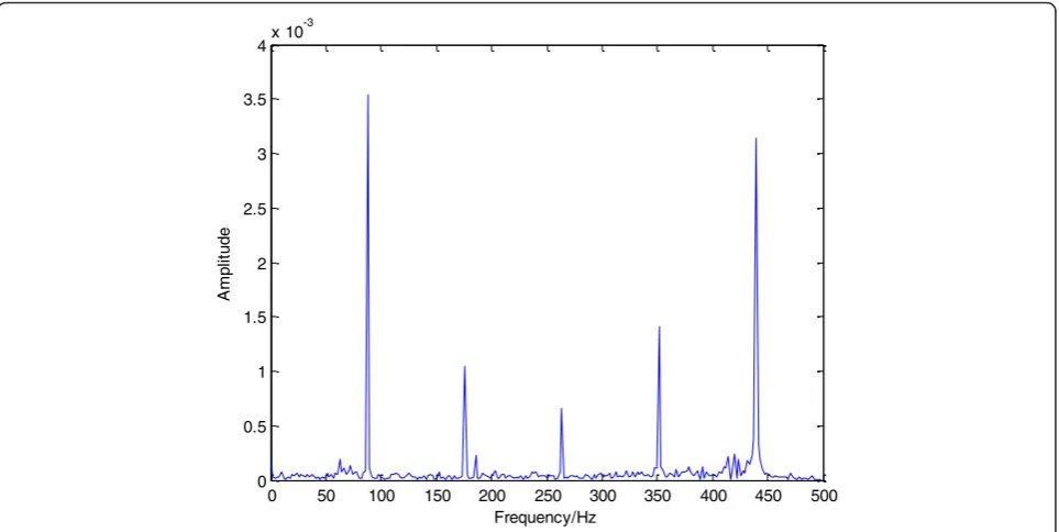
0 50 100 150 200 250 300 350 400 450 500

0 0.5 1 1.5 2 2.5 3 3.5

4x 10 -3

Frequency/Hz

Am

p

lit

u

d

e

3. Experimental verification

Two experimental cases (i) hydraulic pump performance assessment and fault diagnosisand (ii) ball bearing per-formance assessment and fault diagnosis are presented to validate the effectiveness and practicality of applying the proposed method to performance assessment and fault diagnosis of rotating machinery equipment. The description of these case studies will follow the se-quence: (1) experimental setup and data acquisition; (2) signal analysis and feature extraction; (3) analysis of performance assessment and fault diagnosis results.

3.1. Performance assessment and fault diagnosis for hydraulic pump

The hydraulic pump is the heart of a hydraulic system, which determines whether the whole system can run normally or not. Therefore, performance assessment and fault diagnosis of the hydraulic pump is of great import-ance. Usually, when a hydraulic pump is under an ab-normal state, it will be revealed by changes of vibration.

Because most mechanical faults are reflected by vibra-tion [33], the vibravibra-tion signals of the hydraulic pump are collected and analyzed in this experiment for perform-ance assessment and fault diagnosis.

3.1.1. Experimental setup and data acquisition

In this experiment, a hydraulic pump was tested and ana-lyzed, as shown in Figure 6. Two commonly occurring faults in hydraulic pumps were set: slipper loose and valve plate wear. Under different states (normal, faults), moni-toring data (vibration signal) were, respectively, acquired from the hydraulic pump end using an acceleration trans-ducer, with motor speed stabilized at 528 rpm, and a sam-pling frequency of 1000 Hz.

3.1.2. Feature extraction by WPA

To determine the wavelet packet decomposition scale, FFT was implemented for the vibration signals acquired under normal, slipper loose, and valve plate wear states. Through the analysis of the frequency spectrum, as shown Table 1 Feature vector samples for learning (hydraulic pump)

Number 1 2 3 4 5 6 7 8

Normal_1 0.0304 0.8484 0.1399 0.3570 0.1182 0.1565 0.1143 0.2843

Normal_2 0.0343 0.8433 0.1396 0.3557 0.1061 0.1819 0.1085 0.2926

Normal_3 0.0305 0.8307 0.1360 0.3732 0.1231 0.1659 0.1228 0.3057

Normal_4 0.0280 0.8163 0.1654 0.3778 0.1183 0.1491 0.1432 0.3256

Fault1_1 0.0256 0.8182 0.0260 0.1312 0.3582 0.4088 0.0290 0.1255

Fault1_2 0.0329 0.8141 0.0310 0.1312 0.3450 0.4265 0.0355 0.1255

Fault1_3 0.0355 0.8256 0.0378 0.1357 0.3483 0.3972 0.0323 0.1309

Fault1_4 0.0329 0.8266 0.0358 0.1284 0.3950 0.3517 0.0341 0.1304

Fault2_1 0.0261 0.2428 0.5679 0.0871 0.0190 0.0361 0.7785 0.0507

Fault2_2 0.0156 0.2385 0.5717 0.0861 0.0229 0.0366 0.7775 0.0484

Fault2_3 0.0193 0.2405 0.5628 0.0862 0.0278 0.0283 0.7834 0.0488

Fault2_4 0.0116 0.2479 0.5393 0.0816 0.0275 0.0319 0.7977 0.0521

Table 2 Feature vector samples for testing (hydraulic pump)

Number 1 2 3 4 5 6 7 8

N_1 0.0428 0.8110 0.1647 0.4138 0.1297 0.1359 0.1495 0.2908

N_2 0.0300 0.8195 0.1626 0.4070 0.1180 0.1437 0.1434 0.2833

N_3 0.0353 0.8078 0.1836 0.4182 0.1089 0.1534 0.1464 0.2841

N_4 0.0326 0.8142 0.1716 0.4177 0.1107 0.1467 0.1538 0.2732

F1_1 0.0293 0.8259 0.0367 0.1255 0.4254 0.3138 0.0316 0.1397

F1_2 0.0243 0.8344 0.0266 0.1398 0.3832 0.3446 0.0229 0.1295

F1_3 0.0318 0.8399 0.0281 0.1274 0.3242 0.3902 0.0266 0.1356

F1_4 0.0360 0.8293 0.0338 0.1308 0.4289 0.2984 0.0237 0.1383

F2_1 0.0088 0.2475 0.5249 0.0839 0.0189 0.0374 0.8075 0.0484

F2_2 0.0185 0.2501 0.5710 0.0907 0.0299 0.0232 0.7739 0.0511

F2_3 0.0095 0.2463 0.5446 0.0841 0.0256 0.0263 0.7945 0.0541

in Figures 7 and 8, it can be seen that there are clear peaks appearing evenly at six characteristic frequencies. Further-more, the normal signal and fault (slipper loose) signal have distinctively different peaks at the six characteristic frequencies. Therefore, each set of acquired vibration sig-nals is suitable to be decomposed into eight frequency bands by three-layer wavelet packet decomposition. In that way, all the peaks can be contained in different fre-quency bands. Then, an eight-dimensional feature vector can be constructed by calculating and normalizing the en-ergy of each band. The frequency range corresponding to each frequency band is (nωmax/2N, (n+ 1)ωmax/2N), where

N= 3,n= 0, 1,. . .,7, andωmaxis the maximum frequency; hereωmax= 498.

For those three states, eight feature vector samples were acquired, respectively. The first four samples of each state were used as the FDA learning set (for clearer identifica-tion they were numbered as Normal_1 to Normal_4, Fault1_1 to Fault1_4, and Fault2_1 to Fault2_4, corre-sponding to the normal state, slipper loose state, and valve plate wear conditions, respectively), while the others were used as the testing set (they were also numbered in the same manner as: N_1 to N_4, F1_1 to F1_4, and F2_1 to F2_4, respectively).

The feature vector samples for learning and testing are shown in Tables 1 and 2.

3.1.3. Analysis of states separability

In order to demonstrate the separability of feature vector samples acquired during normal, slipper loose, and valve plate wear states, HCA was selected and carried out on the learning set. As shown in Figure 9, the tree dendrogram

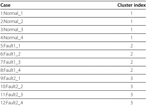
clearly shows the whole process of clustering. First, each sample was taken as a class. After the first clustering, according to the distance between classes, samples Fault2_1 to Fault2_4 were merged into a cluster, samples Normal_1 to Normal_4 were merged into another cluster, and samples Fault1_1 to Fault1_4 were merged into the third cluster. Moreover, from the cluster membership, as shown in Table 3, it was found that all the normal samples gathered in cluster 1, all the slipper loose samples gathered in cluster 2, and all the valve plate wear samples gathered in cluster 3. The results are consistent perfectly with the practical situation, and can be seen as strong evidence for the separability of the different states.

Figure 9A tree dendrogram of HCA (hydraulic pump).

Table 3 Clustering membership of learning set (hydraulic pump)

Case Cluster index

1:Normal_1 1

2:Normal_2 1

3:Normal_3 1

4:Normal_4 1

5:Fault1_1 2

6:Fault1_2 2

7:Fault1_3 2

8:Fault1_4 2

9:Fault2_1 3

10:Fault2_2 3

11:Fault2_3 3

3.1.4. Analysis of performance assessment results

In this study, for the purpose of performance assess-ment, the normal samples numbered as Normal_1 to Normal_4 were used to construct and characterize the normal population noted asG_N. Through FDA, a space conversion method was achieved, by which, the different populations and the new measurement data can be pro-jected from the original eight-dimensional space into a new two-dimensional space.

Then, the MDs between the normal populationG_Nand those samples included in the testing set, as shown in Table 2, were calculated. They were transformed into nor-malized CVs according to formula (13). The MD and CV curves are shown in Figures 10 and 11. Obviously, con-trasting with the MDs of the normal testing samples, the MDs of the slipper loose and valve plate wear testing sam-ples were quite large, because the normal testing samsam-ples were located nearby the normal populationG_N, while the

0 2 4 6 8 10 12

0 0.5 1 1.5 2 2.5 3 3.5 4 4.5 5

Sample

MD

Figure 10MD result of testing set (hydraulic pump).

0 2 4 6 8 10 12

0.4 0.5 0.6 0.7 0.8 0.9 1

Sample

CV

fault testing samples were located far away, i.e., the slipper loose and valve plate wear samples were in an abnormal condition. Conversely, the CVs of the normal testing sam-ples were relatively high; close to 0.9. Whereas the CVs of the fault testing samples were all quite low; falling below the presupposed threshold of 0.6. Therefore, the CV index indicated that the normal testing samples were in a normal condition; while the slipper loose and valve plate wear test-ing samples were in a faulty condition. The analysis demonstrated that the performance assessment could be quantized and visualized by MD and CV, and coupled with a presupposed threshold where abnormal states can be detected. Therefore, this is a successful trial of the per-formance assessment and fault detection.

3.1.5. Analysis of fault diagnosis results

As previously mentioned in the performance assessment analysis, the samples in the testing set (numbered as F1_1 to F1_4 and F2_1 to F2_4) were detected as fault states. To identify which type of fault they belonged to, as a refer-ence, the normal samples in the testing set (numbered as N_1 to N_4) were also considered. The MDs between those samples in the testing set and these three popula-tions were calculated, as shown in Table 4. In order to fa-cilitate analysis, the normal population was noted asG_N, the slipper loose and valve plate wear state populations were noted as G_F1 and G_F2, respectively. Through

comparative analysis, the samples under normal condi-tions had the smallest MDs with the population G_N, while the samples under slipper loose condition and valve plate wear condition had the smallest MDs with the popu-lationG_F1 andG_F2, respectively, as shown in the‘Min’ row of Table 4. According to the discriminant rule in Sec-tion 2.5, it can be determined that the samples N_1 to N_4 belonged to normal conditions, the samples F1_1 to F1_4 and F2_1 to F2_4 were under slipper loose state and valve plate wear state, respectively, as shown in the‘Mode’ row. This accurate diagnosis result is further proof of the effectiveness of the proposed method in fault diagnosis.

3.2. Performance assessment and fault diagnosis for ball bearing

Bearings are critical components in rotating machines because their failure could lead to serious damage in machines. In recent years, bearing fault diagnosis has received increasing attention [34-36]. In this case, vibra-tion signals are acquired from the ball bearing housing for performance assessment and fault diagnosis.

3.2.1. Experimental setup and data acquisition

In this case study, the test data were acquired from the Case Western Reserve University Bearing Data Center. As shown in Figure 12, the test-rig consists of a 2-horsepower motor (left), a torque transducer/encoder (center), a N_1 N_2 N_3 N_4 F1_1 F1_2 F1_3 F1_4 F2_1 F2_2 F2_3 F2_4

G_N 0.1490 0.1288 0.0413 0.1135 3.0432 3.0394 3.1073 2.8714 4.9359 4.8058 4.9323 4.9614

G_F1 3.5555 3.5412 3.4477 3.5199 0.3838 0.3794 0.3107 0.5563 7.8717 7.7396 7.8727 7.9023

G_F2 4.7123 4.7364 4.8134 4.7444 7.4089 7.4290 7.5040 7.2451 0.0885 0.0495 0.0928 0.1209

Min 0.1490 0.1288 0.0413 0.1135 0.3838 0.3794 0.3107 0.5563 0.0885 0.0495 0.0928 0.1209

Mode G_N G_N G_N G_N G_F1 G_F1 G_F1 G_F1 G_F2 G_F2 G_F2 G_F2

dynamometer (right), and control electronics (data not shown). The test bearings support the motor shaft. Sin-gle point faults were introduced separately at the inner-race, outer-inner-race, and rolling element (i.e., ball) of the test bearing using electro-discharge machining with fault diameters of 7 mm. Faulted bearings were reinstalled into the test motor, and vibration data were recorded under different four states (normal, faults) using ac-celerometers, with motor loads of 2 horsepower, mo-tor speed of 1750 rpm, and a sampling frequency of 12,000 Hz.

3.2.2. Feature extraction by WPA

Through implementation of FFT on the acquired vibra-tion data, it was found that the characteristic frequencies under normal, inner-race fault, outer-race fault, and ball fault states are distributed separately in different fre-quency bands, and that there is little overlap between any two adjacent frequencies in the spectrum. Therefore, three-layer wavelet packet decomposition can also be ap-plied to the vibration data, and thus, eight-dimensional feature vectors can be acquired by calculating and nor-malizing the energy of each band.

Table 5 Feature vector samples for learning (rolling bearing)

Number 1 2 3 4 5 6 7 8

N_1 0.8111 0.5012 0.0524 0.2964 0.0002 0.0018 0.0053 0.0187

N_2 0.8259 0.4665 0.0544 0.3112 0.0002 0.0019 0.0054 0.02

N_3 0.7891 0.5274 0.0524 0.3097 0.0002 0.0018 0.0053 0.0204

N_4 0.8137 0.493 0.0553 0.3023 0.0002 0.0018 0.0056 0.0194

I_1 0.0795 0.2297 0.5852 0.1497 0.0014 0.0081 0.7446 0.1471

I_2 0.0823 0.2226 0.5831 0.1464 0.0015 0.0082 0.7467 0.157

I_3 0.081 0.2341 0.6031 0.1474 0.0014 0.0084 0.7306 0.1388

I_4 0.0723 0.2279 0.5922 0.1505 0.0014 0.0092 0.7412 0.1417

O_1 0.0069 0.0096 0.4907 0.0156 0.0082 0.0137 0.8681 0.0707

O_2 0.0065 0.0096 0.4945 0.0161 0.0081 0.0137 0.8655 0.0759

O_3 0.0069 0.0098 0.4831 0.0145 0.0076 0.0121 0.8725 0.0696

O_4 0.0065 0.01 0.5217 0.016 0.007 0.0124 0.8492 0.0777

B_1 0.045 0.0449 0.4876 0.0184 0.0005 0.0027 0.8703 0.0181

B_2 0.0443 0.0424 0.457 0.0189 0.0005 0.0025 0.887 0.0179

B_3 0.0426 0.0436 0.464 0.0187 0.0005 0.0025 0.8833 0.0186

B_4 0.0412 0.042 0.4584 0.0179 0.0004 0.0022 0.8865 0.0175

Table 6 Feature vector samples for testing (rolling bearing)

Number 1 2 3 4 5 6 7 8

N_T1 0.804 0.5112 0.0511 0.2987 0.0002 0.0016 0.0051 0.0192

N_T2 0.8119 0.5007 0.0528 0.2948 0.0002 0.0018 0.0053 0.019

N_T3 0.8208 0.4824 0.0538 0.3006 0.0002 0.0017 0.0055 0.0194

N_T4 0.7854 0.5344 0.0532 0.307 0.0002 0.0018 0.0054 0.0198

I_T1 0.0734 0.2138 0.58 0.1423 0.0015 0.008 0.7556 0.1461

I_T2 0.087 0.2276 0.5929 0.15 0.0014 0.0089 0.7394 0.1403

I_T3 0.0769 0.2242 0.6017 0.1463 0.0016 0.0084 0.7343 0.1454

I_T4 0.071 0.2271 0.5888 0.1535 0.0014 0.0082 0.7421 0.1498

O_T1 0.0066 0.0091 0.4939 0.0159 0.0073 0.0132 0.8661 0.0736

O_T2 0.0073 0.0098 0.4945 0.0166 0.0075 0.0128 0.8655 0.0759

O_T3 0.0068 0.0108 0.5057 0.0159 0.0073 0.0137 0.8594 0.0706

O_T4 0.0069 0.0098 0.4976 0.0154 0.0077 0.0133 0.8642 0.0705

B_T1 0.0438 0.0431 0.483 0.0187 0.0005 0.0024 0.8731 0.0188

B_T2 0.0438 0.0439 0.4753 0.018 0.0006 0.0026 0.8773 0.018

B_T3 0.046 0.0411 0.471 0.0197 0.0005 0.0023 0.8796 0.0176

For those four states, eight feature vector samples were acquired. The first four samples of each state were used as the FDA learning set (for clearer identification they were numbered as N_1 to N_4, I_1 to I_4, O_1 to O_4, and B_1 to B_4, corresponding to the normal state, inner-race fault state, outer-race fault state, and ball fault state, respect-ively), while the others were used as the testing set (they were also numbered in the same manner as N_T1 to N_T4, I_T1 to I_T4, O_T1 to O_T4, and B_T1 to B_T4, respectively).

The feature vector samples for learning and testing are shown in Tables 5 and 6.

3.2.3. Analysis of states separability

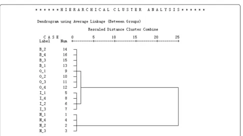
The HCA was applied to the learning set, as shown in Figure 13, and the whole process of clustering was dis-played in a tree dendrogram. First, each sample was taken as a class. After the first clustering, according to the distance between classes, samples B_1 to B_4 and samples O_1 to O_4 were merged into a cluster, samples I_1 to I_4 were merged into another cluster, and samples N_1 to N_4 were merged into the third cluster. As shown in Table 7, the cluster membership was that all the normal samples gathered in cluster 1, all the inner-race fault samples gathered in cluster 2, all the outer-race fault samples gathered in cluster 3, and all the ball fault sam-ples gathered in cluster 4. The outputs of SPSS Statistics, the tree dendrogram, and the cluster membership table

successfully demonstrated the separability of feature vec-tor samples acquired during those four conditions.

3.2.4. Analysis of performance assessment results

In this study, the normal samples numbered N_1 to N_4 were used to construct and characterize the normal population noted as G_N. Through FDA, the original Figure 13A tree dendrogram of HCA (rolling bearing).

Table 7 Clustering memberships of learning set (rolling bearing)

Case Cluster index

1:N_1 1

2:N_2 1

3:N_3 1

4:N_4 1

5:I_1 2

6:I_2 2

7:I_3 2

8:I_4 2

9:O_1 3

10:O_2 3

11:O_3 3

12:O_4 3

13:B_1 4

14:B_2 4

15:B_3 4

eight-dimensional space was projected into a new three-dimensional space.

The MDs between the normal population G_N and those samples included in the testing set, as shown in Table 6, were calculated and transformed into normalized CVs according to formula (13). The MD and CV curves are shown in Figures 14 and 15. Apparently, the MDs of the normal testing samples were quite low, while those of the fault testing samples were quite large. Because the normal testing samples were located nearby the normal

population G_N, while the inner-race fault, outer-race fault, and ball fault testing samples were located far away. Conversely, the CVs of the normal samples were relatively large, whereas the CVs of all fault testing samples were quite low, falling below the presupposed threshold of 0.6. Thus, it indicated that the inner-race fault, outer-race fault, and ball fault samples were in a faulty condition. Therefore, this result demonstrated that the performance assessment of ball bearing can be quantized and visualized by MD and CV.

0 2 4 6 8 10 12 14 16

0 2 4 6 8 10 12

Sample

MD

Figure 14MD result of testing set (rolling bearing).

0 2 4 6 8 10 12 14 16

0.4 0.5 0.6 0.7 0.8 0.9 1

Sample

CV

3.2.5. Analysis of fault diagnosis results

In the performance assessment analysis, the CVs of the samples in the testing set (numbered as I_T1 to I_T4, O_T1 to O_T4, and B_T1 to B_T4) were quite low, so they were in fault states. To identify which type of fault they belonged to, as a reference, the normal samples in the testing set (numbered as N_T1 to N_T4) were also considered, the MDs between the samples in the testing set and those four populations were calculated, as shown in Table 8. In order to facilitate analysis, the normal population was noted as G_N, the inner-race-fault, outer-race-fault, and ball fault populations were noted as G_I, G_O, and G_B, respectively. Through comparative analysis, the samples under normal conditions had the smallest MDs with the population G_N, while the sam-ples under inner-race-fault, outer-race-fault, and ball fault conditions had the smallest MDs with the popula-tion G_I, G_O, and G_B, respectively, as shown in the

‘Min’ row of Table 8. Therefore, it can be determined that the samples N_T1 to N_T4 belonged to normal condition, the samples I_T1 to I_T4, O_T1 to O_T4, and B_T1 to B_T4 were under inner-race fault condi-tion, outer-race fault condicondi-tion, and ball fault condicondi-tion, respectively, as shown in the ‘Mode’ row. This accurate diagnosis result is further proof of the effectiveness of the proposed method in fault diagnosis.

4. Conclusion

In this article, addressing the challenging issues on per-formance assessment, fault detection, and fault diagnosis, a novel method based on FDA and MD is introduced, and an integrated framework for performance assessment, fault detection, and fault diagnosis is built.

In this method, FDA is applied as an optimal linear di-mensionality reduction technique, in terms of maximizing

the separation between different populations. In the new low-dimensional space, MD, which can be transformed into normalized CV, is calculated for performance assess-ment, and abnormal states can be detected with the pre-supposed threshold. Furthermore, once various fault data are available, the unknown fault mode can be identified accurately by comparing the MDs between the new data and each normal/fault population.

However, how to transform MD into CV for perform-ance assessment and to determine an adaptive threshold for fault detection is still a challenge for future work. In the future, we are going to acquire sequential online deg-radation measurements for real-time performance degra-dation assessment and detection, and enlarge the number of fault and learning samples for more accurate fault diag-nosis. Moreover, we plan to apply this approach to differ-ent compondiffer-ents, such as gearboxes, shafts, etc., to further verify the effectiveness and evaluate the possibility of ge-neralizing the proposed approach.

Competing interests

The authors declare that they have no competing interests.

Authors’contributions

XCT carried out the performance assessment studies, and drafted the manuscript; CL (Corresponding author) carried out the diagnosis studies, and participated in the algorithm design and manuscript revision; CL and ZLW carried out the preparation of experimental data, and participated in the algorithm design. All authors read and approved the final manuscript.

Acknowledgements

This research was supported by the National Natural Science Foundation of China (Grant nos.61074083, 50705005, and 51105019) as well as the Technology Foundation Program of National Defense (Grant no. Z132010B004). The authors are very grateful for the valuable suggestions from the reviewers and editor.

Received: 7 May 2012 Accepted: 2 December 2012 Published: 10 January 2013

N_T1 N_T2 N_T3 N_T4 I_T1 I_T2 I_T3 I_T4

G_N 0.0245 0.0249 0.0352 0.1014 10.3384 10.3041 10.3426 10.2988

G_I 10.3123 10.3094 10.3010 10.3022 0.1079 0.0547 0.0639 0.0609

G_O 10.8671 10.8645 10.8462 10.8709 1.8074 1.9666 1.8590 1.8561

G_B 10.6774 10.6747 10.6590 10.6777 1.2993 1.4575 1.3519 1.3486

Min 0.0245 0.0249 0.0352 0.1014 0.1079 0.0547 0.0639 0.0609

Mode G_N G_N G_N G_N G_I G_I G_I G_I

O_T1 O_T2 O_T3 O_T4 B_T1 B_T2 B_T3 B_T4

G_N 10.8419 10.8391 10.8812 10.8567 10.7244 10.6955 10.6792 10.6498

G_I 1.9145 1.9065 1.9045 1.9098 1.4065 1.3990 1.4010 1.4045

G_O 0.0122 0.0141 0.0358 0.0078 0.5250 0.5308 0.5288 0.5272

G_B 0.5243 0.5168 0.5168 0.5198 0.0642 0.0362 0.0181 0.0150

Min 0.0122 0.0141 0.0358 0.0078 0.0642 0.0362 0.0181 0.0150

References

1. J Lee, J Ni, D Djurdjanovic, H Qiu, HT Liao, Intelligent prognostics tools and e-maintenance. Comput. Ind.57, 476–489 (2006). doi:10.1016/j. compind.2006.02.014

2. AKS Jardine, D Lin, D Banjevic, A review on machinery diagnostics and prognostics implementing condition-based maintenance. Mech. Syst. Signal Process.20, 1483–1510 (2006). doi:10.1016/j.ymssp. 2005.09.012

3. A Heng, S Zhang, ACC Tan, J Mathew, Rotating machinery prognostics: state of the art, challenges and opportunities. Mech. Syst. Signal Process. 23, 724–739 (2009). doi:10.1016/j.ymssp. 2008.06.009

4. HP Bloch, FK Geitner,Practical Machinery Management for Process Plants. Machinery Failure Analysis and Trouble Shooting, vol. 2, 3rd edn. (Gulf Professional Publishing, Houston, 1997)

5. WB Wang, Modelling the probability assessment of system state using available condition information. IMA J. Manage. Math.17(3), 225_–234 (2006). doi:10.1093/imaman/dpi035

6. WB Wang, A two-stage prognosis model in condition based maintenance. Eur. J. Oper. Res.182, 1177_–1187 (2007). doi:10.1016/j.ejor.2006.08.047 7. LL Ma, Z Zhang, JZ Wang, Combination method of support vector machine

and fisher discriminant analysis for chemical process fault diagnosis, in

Paper presented at the 29th Chinese Control Conference(Beijing, 2010),

pp. 4000–4003

8. LH Chiang, ME Kotanchek, AK Kordon, Fault diagnosis based on Fisher discriminant analysis and support vector machines. Comput. Chem. Eng. 28, 1389–1401 (2004). doi:10.1016/j.compchemeng.2003.10.002 9. QP He, SJ Qin, J Wang, A new fault diagnosis method using fault

directions in Fisher discriminant analysis. AICHE J.51(2), 555_–571 (2005). doi:10.1002/aic.10325

10. XB He, W Wang, YP Yang, YH Yang, Variable-weighted Fisher discriminant analysis for process fault diagnosis. J. Process. Control.19, 923–931 (2009). doi:10.1016/j.jprocont.2008.12.001

11. MJ Fuente, D Garcia-Alvarez, GI Sainz-Palmero, Fault detection and identification method based on multivariate statistical techniques, inPaper presented at the Proceedings of Emerging Technologies & Factory Automation (Mallorca, 2009), pp. 1–6

12. LX Liao, J Lee, Design of a reconfigurable prognostics platform for machine tools. Expert Syst. Appl.37, 240–252 (2010). doi:10.1016/j.eswa.2009.05.004 13. I Gurrutxaga, I Albisua, O Arbelaitz, JI Martin, J Muguerza, JM Perez, I Perona,

An efficient method to find the best partition in hierarchical clustering based on a new cluster validity index. Pattern Recognit43, 3364–3373 (2010). doi:10.1016/j.patcog.2010.04.021

14. J Goldberger, T Tassa, A hierarchical clustering algorithm based on the Hungarian method. Pattern Recognit. Lett.29(11), 1632_–1638 (2008). doi:10.1016/j.patrec.2008.04.003

15. M Safayani, MTM Shalman, Matrix-variate probabilistic model for canonical correlation analysis. EURASIP J. Adv. Signal Process.7, (2011). Article ID 748430 16. A Eftekhari, HA Moghaddam, M Forouzanfar, J Alirezaie, Incremental local

linear fuzzy classifier in fisher space. EURASIP J. Adv. Signal Process., (2009). Article ID 360834

17. LX Liao,An Adaptive Modeling for Robust Prognostics on a Reconfigurable Platform. PhD, University of Cincinnati, Engineering: Industrial Engineering (University of Cincinnati, Cincinnati, 2010)

18. XZ Zhao, BY Ye, Convolution wavelet packet transform and its applications to signal processing. Dig. Signal Process.20, 1352–1364 (2010). doi:10.1016/j. dsp. 2010.01.007

19. JD Wu, CH Liu, An expert system for fault diagnosis in internal combustion engines using wavelet packet transform and neural network. Expert Syst. Appl.36, 4278_–4286 (2009). doi:10.1016/j.eswa.2008.03.008

20. YN Pan, J Chen, XL Li, Bearing performance degradation assessment based on lifting wavelet packet decomposition and fuzzy c-means. Mech. Syst. Signal Process.24, 559–566 (2010). doi:10.1016/j.ymssp. 2009.07.012 21. B Kotnik, Z Kacic, A comprehensive noise robust speech parameterization

algorithm using wavelet packet decomposition-based denoising and speech feature representation techniques. EURASIP J. Adv. Signal Process., (2007). Article ID 64102

22. G Forestier, C Wemmert, P Gancarski, Multisource images analysis using collaborative clustering. EURASIP J. Adv. Signal Process., (2008). Art ID 374095

23. ZS Wang, A Maier, NK Logothetis, HL Liang, Single-trial classification of bistable perception by integrating empirical mode decomposition,

clustering, and support vector machine. EURASIP J. Adv. Signal Process., (2008). Article ID 592742

24. I Kojadinovic, Hierarchical clustering of continuous variables based on the empirical copula process and permutation linkages. Comput. Stat. Data Anal.54, 90–108 (2010). doi:10.1016/j.csda.2009.07.014

25. JAS Almeida, LMS Barbosa, AACC Pais, SJ Formosinho, Improving hierarchical cluster analysis: a new method with outlier detection and automatic clustering. Chemometrics Int. Lab. Syst.87, 208–217 (2007). doi:10.1016/j.chemolab.2007.01.005

26. ML Song, YQ Song, HY Yu, ZY Wang, Calculation of China’s environmental efficiency and relevant hierarchical cluster analysis from the perspective of regional differences. Math. Comput. Model., (2012). doi:10.1016/j.mcm. 2012.04.003

27. C Bouveyron, C Brunet, Probabilistic Fisher discriminant analysis: a robust and flexible alternative to Fisher discriminant analysis. Neurocomputing 90, 12–22 (2012). doi:10.1016/j.neucom.2011.11.027

28. R Khemchandani, Jayadeva, S Chandra, Learning the optimal kernel for Fisher discriminant analysis via second order cone programming. Eur. J. Oper. Res.203, 692–697 (2010). doi:10.1016/j.ejor.2009.09.020 29. H Shin, An extension of Fisher’s discriminant analysis for stochastic

processes. J. Multivariate Anal.99, 1191–1216 (2008). doi:10.1016/j. jmva.2007.08.001

30. CR Rao,Linear Statistical Inference and Its Application, 2nd edn. (Wiley, New York, 1973)

31. A Heng, A Tan, J Mathew, BS Yang, Machine prognosis with full utilization of truncated lifetime data, inProceedings of the Second World Congress on

Engineering Asset Management(, Harrogate, 2007), pp. 775–784

32. G Niu, S Singh, SW Holland, M Pecht, Health monitoring of electronic products based on Mahalanobis distance and Weibull decision metrics. Microelectron. Reliab.51, 279–284 (2011). doi:10.1016/j.microrel.2010.09.009 33. JP Wang, HT Hu, Vibration-based fault diagnosis of pump using fuzzy

technique. Measurement39, 176–185 (2006). doi:10.1016/j. measurement.2005.07.015

34. S Prabhakar, AR Mohanty, AS Sekhar, Application of discrete wavelet transform for detection of ball bearing race faults. Tribol. Int.35(12), 793–800 (2002) 35. KF Al-Raheem, A Roy, KP Ramachandran, DK Harrison, S Grainger, Rolling

element bearing fault diagnosis using Laplace-Wavelet envelope power spectrum. EURASIP J. Adv. Signal Process., (2007). Article ID 073629 36. A Ibrahim, F Bonnardot, M El Badaoui, F Guillet, Detection of bearing

damage using stator current, and voltage to cancel electrical noise. EURASIP J. Adv. Signal Process., (2011). Article ID 235236

doi:10.1186/1687-6180-2013-5

Cite this article as:Taoet al.:An approach to performance assessment and fault diagnosis for rotating machinery equipment.EURASIP Journal on Advances in Signal Processing20132013:5.

Submit your manuscript to a

journal and benefi t from:

7Convenient online submission

7Rigorous peer review

7Immediate publication on acceptance

7Open access: articles freely available online

7High visibility within the fi eld

7Retaining the copyright to your article