Managing Algorithmic Skeleton Nesting Requirements
in Realistic Image Processing Applications: The Case of
the SKiPPER-II Parallel Programming Environment’s
Operating Model
R ´emi Coudarcher,1Florent Duculty,2Jocelyn Serot,2Fr ´ed ´eric Jurie,2Jean-Pierre Derutin,2and
Michel Dhome2
1Projet OASIS, INRIA Sophia-Antipolis, 2004 route des Lucioles, BP 93, 06902 Sophia-Antipolis Cedex, France Email:[email protected]
2LASMEA (UMR 6602 UBP/CNRS), Universit´e Blaise-Pascal-(Clermont II), Campus Universitaire des C´ezeaux, 24 avenue des Landais, 63177 Aubiere Cedex, France
Emails:[email protected],[email protected],[email protected], [email protected],[email protected]
Received 5 September 2003; Revised 17 August 2004
SKiPPER is a Skeleton-based Parallel Programming EnviRonment being developed since 1996 and running at LASMEA Labo-ratory, the Blaise-Pascal University, France. The main goal of the project was to demonstrate the applicability of skeleton-based parallel programming techniques to the fast prototyping of reactive vision applications. This paper deals with the special fea-tures embedded in the latest version of the project: algorithmic skeleton nesting capabilities and a fully dynamic operating model. Throughout the case study of a complete and realistic image processing application, in which we have pointed out the requirement for skeleton nesting, we are presenting the operating model of this feature. The work described here is one of the few reported experiments showing the application of skeleton nesting facilities for the parallelisation of a realistic application, especially in the area of image processing. The image processing application we have chosen is a 3D face-tracking algorithm from appearance.
Keywords and phrases:parallel programming, image processing, algorithmic skeleton, nesting, 3D face tracking.
1. INTRODUCTION
At Laboratoire des Sciences et Mat´eriaux pour l’Electroni-que, et d’Automatique (LASMEA), the Blaise-Pascal Univer-sity’s laboratory of electrical engineering, France, we have been developing since 1996 a parallel programming envi-ronment, called SKiPPER (SKeleton-based Parallel Program-ming EnviRonment), based on the use of algorithmic skele-tons to provide application programmers with a mostly au-tomatic procedure for designing and implementing paral-lel applications. The SKiPPER project was originally envi-soned to build realistic vision applications for embedded platforms.
Due to the features in the latest developed version of SKiPPER, called SKiPPER-II, it has now turned into a more usable parallel programming environment addressing PC cluster architectures and different kinds of applications as well.
The reason to develop such an environment is that, re-lying on parallel machines, programmers are facing several
difficulties. Indeed, in the absence of high-level parallel pro-gramming models and environments, they have to explicitly take into account every aspect of parallelism such as task partitioning and mapping, data distribution, communica-tion scheduling, or load balancing. Having to deal with these low-level details results in long, tedious, and error-prone de-velopment cycles,1 thus hindering a true experimental
ap-proach. Parallel programming at a low level of abstraction also limits code reusability and portability. Our environment finally tries to “capture” the expertise gained by program-mers when implementing vision applications using low-level parallel constructs, in order to make it readily available to al-gorithmists and image processing specialists. That is the rea-son why SKiPPER takes into account low-level implementa-tion details such as task partiimplementa-tioning and mapping, commu-nication scheduling, or load balancing.
(a) (b) (c) (d)
Figure1: The four skeletons of SKiPPER are, from left to right, split-compute-merge skeleton, data farming skeleton, task farming skeleton, and iteration with memory skeleton.
The SKiPPER-I suite of tools, described in [1,2,3,4], was the first realization of this methodology. It was, however, lim-ited in terms of skeleton composition. In particular, it could not accommodate arbitrary skeleton nesting, that is to say, the possibility for one skeleton to take another skeleton as an argument. The SKiPPER-II implementation [5] was de-veloped to solve this problem. Its main innovative feature is its ability to handle arbitrary skeleton nesting.
Skeleton nesting has always been perceived as a chal-lenge by skeleton implementers and only a few projects have produced working implementations supporting it (see, e.g., [6,7,8]). But most of the applications used in these cases were “toy” programs in which skeleton nesting is a rather “artificial” construct needed for benchmarking purposes. By contrast, we think that showing a realistic application which needs such a facility in order to be parallelised has a great importance in validating the concept.
For these reasons, this paper focuses on the parallelisa-tion, using a set of algorithmic skeletons specifically designed for image processing, of a complete and realistic image pro-cessing application in which we have pointed out require-ments of skeleton nesting. The realistic application we have chosen is a 3D face-tracking algorithm which had been pre-viously developed in our laboratory [9].
The paper is organised as follows.Section 2briefly recalls the skeleton-based parallel programming concepts used in SKiPPER and describes the suite of tools that has been de-veloped. Section 3presents the 3D face-tracking algorithm we used as a realistic case study to be parallelised using the SKiPPER-II environment. Only the main features of the al-gorithm are described here in a way that our design choices (in terms of parallelisation) could be understood. These de-sign choices are described inSection 4. Result analysis can be found inSection 5. FinallySection 6concludes the paper.
2. THE SKiPPER PROJECT
2.1. Skeleton-based parallel programming and SKiPPER-I
Skeleton-based parallel programming methodologies (see [10,11]) provide a way for conciliating fast prototyping and efficiency. They aim at providing user guidance and a mostly automatic procedure for designing and implementing paral-lel applications. For that purpose, they provide a set of
algo-rithmic skeletons, which arehigher-order program constructs encapsulating common and recurrent forms of parallelismto make them readily available for the application programmer. The latter does not have to take into account low-level im-plementation details such as task partitioning and mapping, data distribution, communication scheduling, and load bal-ancing.
The application programmer provides a skeletal struc-tured description of the parallel program, the set of application-specific sequential functions used to instantiate the skeletons, and a description of the target architecture. The overall result is a significant reduction in the design-implement-validate cycle time.
Due to our primary interest in image processing, we have designed and implemented a skeleton-based parallel pro-gramming environment, called SKiPPER, based on a set of skeletons specifically designed for parallel vision applications [1,2,3,4,12]. This library of skeletons was designed from a retrospective analysis of existing parallel code. It includes four skeletons (as shown inFigure 1):
(i) split-compute-merge (SCM) skeleton; (ii) data farming (DF);
(iii) task farming (TF) (a recursive version of the DF skele-ton);
(iv) iteration with memory (ITERMEM).
The SCM skeleton is devoted to regular “geometric” process-ing of iconic data, in which the input set of data is split into a fixed number of subsets, each of them is processed indepen-dently and the final result is obtained by merging the results computed on subsets of the input data (they may overlap). This skeleton is applicable whenever the number of subsets is fixed and the amount of work on each subset is the same, resulting in an even workload. Typical examples include con-volutions, median filtering, and histogram computation.
let scm split comp merge x=
merge (map comp (split x))
let df comp acc xs=
foldll acc (map comp xs)
let rec tf triv solve divide comb xs=
let f x=
if (triv x) then solve x
else tf triv solve divide comb (divide x) in foldll comb (map f xs)
Algorithm1: Declarative semantics of SKiPPER skeletons in Caml.
The TF skeleton may be viewed as a generalisation of the DF one, in which the processing of one data item by a worker may recursively generate new items to be processed. These data items are then returned to the farmer to be added to a queue from which tasks are doled out (hence the nametask farming). A typical application of the TF skeleton is image segmentation using classical recursive divide-and-conquer algorithms.
The ITERMEM skeleton does not actually encapsulate parallel behaviour, but is used whenever theiterativenature of the real-time vision algorithms (i.e., the fact that they do not process single images but continuousstreamsof images) has to be made explicit. A typical situation is when compu-tations on thenth image depend on results computed on the
n−1th (orn−kth).
Each skeleton comes with two semantics: a declarative se-mantics, which gives its “meaning” to the application pro-grammer in an implicitly parallel manner, that is, without any reference to an underlying execution model, and an op-erational semantics which provides an explicitly parallel de-scription of the skeleton.
The declarative semantics of each skeleton is shared by all SKiPPER versions. It is conveyed using the Caml language, using higher-order polymorphic functions. The correspond-ing definitions are given inAlgorithm 1. Potential (implicit) parallelism arises from the use of the “map” and “foldl1” higher-order functions.
The operational semantics of a skeleton varies according to the nature of the intermediate representation used by the CTS.
Using SKiPPER, the application designer
(i) provides the source code of the sequential application-specific functions;
(ii) describes the parallel structure of his application in terms of composition of skeletons chosen in the li-brary.
This description is made by using a subset of the Caml functional language, as shown inAlgorithm 2, where a SCM skeleton is used to express the parallel computation of a his-togram using a geometric partitioning of the input image. In this Algorithm, “row partition,” “seq histo,” “merge histo,” and “display histo” are the application-specific sequential functions (written in C) and “scm” is the above-mentioned skeleton. This Caml program is theskeletal program specifica-tion. In SKiPPER-I, it is turned into executable code by first
let img=read img 512 512 ;;
let histo=scm row partition
seq histo merge histo img ;;
let main=display histo img histo ;;
Algorithm2: A “skeletal” program in Caml.
translating it into a graph of parametric process templates and then mapping this graph onto the target architecture. The SKiPPER suite of tools turn these descriptions into exe-cutable parallel code. The main software components are a li-brary of skeletons, a compile-time system (CTS) for generat-ing the parallel C code, and a run-time system (RTS) provid-ing support for executprovid-ing this parallel code on the target plat-form. The CTS can be further decomposed into a front end, whose goal is to generate a target-independent intermediate representation of the parallel program, and a back-end sys-tem, in charge of mapping this intermediate representation onto the target architecture (see Figure 2). The role of the back-end in the CTS is to map the intermediate representa-tion of the parallel program onto the target architecture. For an MIMD target with distributed memory, for example, this involves finding a distribution of the operations/processes on the processors and a scheduling of the communications on the provided medium (bus, point-to-point links, etc.). The distribution and the scheduling can be static, that is, done at compile time, or dynamic, that is, postponed until run time. Both approaches require some kind of RTS. For static approaches, the RTS can take the form of a reduced set of primitives, providing mechanisms for synchronizing threads of computations and exchanging messages between proces-sors. For dynamic approaches, it must include more sophis-ticated mechanisms for scheduling threads and/or processes and dynamically managing communication buffers for in-stance. For this reason, static approaches generally lead to better (and more predictable) performances. But they may lack expressivity. Dynamic approaches, on the other hand, do not suffer from this limitation but this is generally obtained at the expense of reduced performances and predictability. Depending on the distribution and scheduling technique used in the back-end, the parallel code takes the form of a set of either MPMD (one distinct program per processor) or SPMD (the same program for all processors) programs. These programs are linked with the code of the RTS and the definition of the application-specific sequential functions to produce the executable parallel code.
Completely designed by the end of 1998, SKiPPER-I has already been used for implementing several realistic parallel vision applications, such as connected component labelling [1], vehicle tracking [3], and road tracking/reconstruction [4].
SKL1 SKL2 Skeleton
library
Parallel program description
Application-specific sequential functions PGM=
SKL1( SKL2(f1),
SKL3(f2))
Void f2(· · ·); Void f1(· · ·);
· · ·
Front end
Intermediate representation
Back-end (mapping)
Main (){
· · · }P1.c Pn.c
C compiler P0 P1
P2 P3 Run-time support
.c Target architecture
description
CTS Parallel code
.h .c
Executable parallel codes (SPMD/MPMD)
Figure2: SKiPPER global software architecture.
argument. Arbitrary skeleton nesting raises challenging im-plementation issues as reported in [6,8,13] or [7]. For this reason, SKiPPER-II was designed to support arbitrary nest-ing of skeletons. This implementation is based on a com-pletely revised execution model for skeletons. Its three main features are
(i) the reformulation of all skeletons as instances of a very general one: a new version of the task farming skeleton (called TF/II),
(ii) a fully dynamic scheduling mechanism (scheduling was mainly static in SKiPPER-I),
(iii) a portable implementation of skeletons based on an MPIcommunication layer (seeSection 2.5).
2.2. SKiPPER-II
SKiPPER-I relied on a mostly static execution model for skeletons: most of the decisions regarding distribution of computations and scheduling of communications were made at compile time by a third-party CAD software called Syn-DEx [14]. This implementation path, while resulting in very efficient distributed executives for “static”—by static we mean that the distribution and scheduling of all communi-cations do not depend on input data and can be predicted at compile-time—did not directly support “dynamic” skele-tons, in particular those based on data or task farming (DF and TF). The intermediate representation of DF and TF was therefore rather awkward in SKiPPER-I, relying on ad hoc auxiliary processes and synchronisation barriers to hide dy-namically scheduled communications from the static sched-uler [2].
Another point about the design of SKiPPER-I is that the target executable code was MPMD: the final parallel C code took the form of a set of distinct main functions (one per processor), each containing direct calls to the application-specific sequential functions interleaved with communica-tions.
By contrast, execution of skeleton-based applications in SKiPPER-II is carried out by asingleprogram (the “kernel” in the sequel)—written in C—running in SPMD mode on all processors and ensuring a fullydynamicdistribution and scheduling of processes and communications. The kernel’s work is to
(i) run the application by interpreting an intermediate de-scription of the application obtained from the Caml program source,
(ii) emulate any skeleton of the previous version of SKiP-PER,
(iii) manage resources (processors) for load balancing when multiple skeletons must run simultaneously.
In SKiPPER-II, the target executable code is therefore built from the kernel and the application-specific sequential func-tions. Indeed, the kernel acts as a small (distributed) operat-ing system that provides all routines the application needs to run on a processor network.
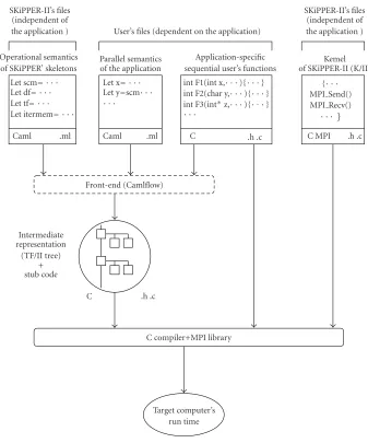
The overall software architecture of the SKiPPER-II pro-gramming environment is given in Figure 3. The skeletal specificationin Caml is analysed to produce the intermedi-ate description which is interpreted at run time by the kernel; the sequential functions and the kernel code are compiled to-gether to make the target executable code. These points will be detailed in the next sections.
2.3. Intermediate description
Clearly, the validity of the “kernel-based” approach pre-sented above depends on the definition of an adequate in-termediate description. It is the interpretation (at run time) of this description by the kernel that will trigger the execu-tion of the applicaexecu-tion-specific sequential funcexecu-tions on the processors, according to the data dependencies encoded by the skeletons.
A key point about SKiPPER-II is that, at this intermedi-ate level of description, all skeletons have been turned into instancesof a more general one called TF/II. The operational semantics of the TF/II skeleton is similar to the one of DF and TF: a master(farmer) process still doles out tasks to a pool ofworker (slave) processes, but the tasks can now be different (i.e., each worker can compute a different func-tion).
SKiPPER-II’s files (independent of
the application ) User’s files (dependent on the application)
SKiPPER-II’s files (independent of the application ) Operational semantics
of SKiPPER’ skeletons
Parallel semantics of the application
Application-specific sequential user’s functions
Kemel of SKiPPER-II (K/II) Let scm= · · ·
Let df= · · ·
Let tf= · · ·
Let itermem= · · ·
Caml .ml
Let x= · · ·
Let y=scm· · · · · ·
Caml .ml C .h .c
int F1(int x,· · ·){· · · }
int F2(char y,· · ·){· · · }
int F3(int∗z,· · ·){· · · } · · ·
{· · ·
MPI Send() MPI Recv()
· · ·}
Front-end (Camlflow)
Intermediate representation
(TF/II tree) + stub code
C .h .c
C compiler+MPI library
Target computer’s run time
C MPI .h .c
Figure3: SKiPPER-II environment.
(i) First, it makes skeleton composition easier, because the number of possible combinations now reduces to three (TF/II followed by TF/II, TF/II nested in TF/II, or TF/II in parallel with TF/II).
(ii) Second, it greatly simplifies the structure of the run-time kernel, which only has to know how to run a TF/II skeleton.
(iii) Third, there is only one skeleton code to design and maintain, since all other skeletons will be defined in terms of this generic skeleton.
The above-mentioned transformation is illustrated in Figure 4 with a SCM skeleton. In this figure, white boxes represent pure sequential functions and grey boxes repre-sent “support” processes (parameterised by sequential func-tions). Note that at the Caml level, the programmer still uses distinct skeletons (SCM, DF, TF, ITERMEM) when writing
the skeletal description of his application.2The
transforma-tion is done by simply providing alternative definitransforma-tions of the SCM, DF, TF, and so forth higher-order functions in terms of the TF/II one. Skeleton composition is expressed by normal functional composition. The program description appearing inFigure 5, for example, can be written as inAlgorithm 3in Caml.
The intermediate description itself—as interpreted by the kernel—is a tree of TF/II descriptors, where each node contains informations to identify the next skeleton and to re-trieve the C function run by a worker process.Figure 5shows an example of the corresponding data structure in the case of two nested SCM skeletons.
I S
F F F
M O
I S/M O
F F F
SCM TF/II
I: Input function O: Output function S: Split function
M: Merge function F: Compute function
TF/II
Figure4: SCM→TF/II transformation.
2.4. Operating model
Within our fully dynamic operating/execution model, skele-tons are viewed as concurrent processes competing for re-sources on the processor network.
When a skeleton needs to be run, and because any skele-ton is now viewed as a TF/II instance, a kernel copy acts as the master process of the TF/II. This copy manages all data transfers between the master and the worker (slave) processes of the TF/II. Slave processes are located on resources allo-cated dynamicallyby the master. In this way, kernel copies interact to emulate skeleton behaviour. In this model, ker-nel copies (and then processes) can switch from master to worker behaviour depending only on the intermediate repre-sentation requirement. There is no “fixed” mapping for dy-namic skeletons as in SKiPPER-I. As soon as a kernel copy is released after being involved in the emulation of a skeleton, it can be immediately reused in the emulation of another one. This strongly contributes towards easily managing the load-balancing and then efficiently using the available resources.
This is illustrated inFigure 6with a small program show-ing two nested SCM skeletons. This figure shows the role of each kernel copy (two per processor in this case) in the execu-tion of the intermediate descripexecu-tion resulting from the trans-formation of the SCM skeletons into TF/II ones.
Because any kernel copy knows when and where to start a new skeleton without requiring information from copies, the scheduling of skeletons can be distributed. Each copy of the kernel has its own copy of the intermediate description of the application. This means that each processor can start the necessary skeleton when it is needed because it knows which skeleton has stopped. A new skeleton is started when-ever the previous one (in the intermediate description) ends. The next skeleton is always started on the processor which has run the previous skeleton (because this resource is sup-posed to be free and closer than the others!).
Since we want to target dedicated and/or embedded plat-forms, the kernel was designed to work even if the computing nodes are not able to run more than one process at a time (no need for multitasking).
Finally, in the case of a lack of resources, the kernel is able to run some of the skeletons in a sequential manner, includ-ing the whole application, thus providinclud-ing a straightforward sequential emulation facility for parallel programs.
2.5. Management of communications
The communication layer is based on a reduced set of the MPI [15] library functions (typically MPI SSend or MPI Recv), thus increasing the portability of skeleton-based applications across different parallel platforms [16]. This fea-ture has been taken into account from the very beginning of the kernel’s design of SKiPPER-II. We use only synchronous communication functions; however, asynchronous functions may perform much better in some cases (especially when the platform has a specialised coprocessor for communications and when communications and processing can overlap).
This restriction is a consequence of our original experi-mental platform which did not support asynchronous com-munications. This set of communication functions is the most elementary functions of the MPI toolset which can be implemented onto any kind of parallel computer. In such a way, the portability of SKiPPER-II is increased. Moreover, the usability is also higher due to writing a minimum MPI layer to support the execution of SKiPPER is a straightforward and not time-consuming task.
Multithreads were avoided too. Using multithreads in our first context of development, that is to say, with our first ex-perimental platform was not suitable. This platform did not support multithreads,3giving us the minimal design
require-ment for a full platform compatibility.
2.6. Comparative assessment
Comparatively to the first version of SKiPPER, SKiPPER-II uses a fully dynamic implementation mechanism for skeleton-based programs.
This has several advantages. In terms of expressivity, since arbitrary nesting of skeletons is naturally and fully supported. The introduction of new skeletons is also facili-tated, since it only requires giving their translation in terms of TF/II. Portability of parallel applications across different platforms is extremely high: running an application on a new platform only requires a C compiler and a very small subset of the MPI library (easily written for any kind of parallel plat-form). The approach used also provides automatic load bal-ancing, since all mapping and scheduling decisions are taken at run time, depending on the available physical resources. In a same way, sequential emulation is straight obtained in just running the parallel application on a single processor. This is the harder case of a lack of resources in which the SKiPPER-II’s kernel automatically manages to run application as par-allel as possible, running some part of it in sequential on a single processor in order to avoid to stopping the whole ap-plication.
The counterpart is essentially in terms of efficiency in some cases and mostly predictability. As regards to efficiency,
S1
S2
F2
M2
M1
S3
F3
M3 F3
F2 F2 F2
S2
M2 Sk
elet
on
2:
SCM
Sk
elet
on
1:
(T
F/II)
S1 M1
S2 M2
S2 M2
F2 F2 F2 F2
S3 M3
F3 F3 Original application
using 3 SCM skeletons with 2 of them nested
Sk
elet
on
3:
(T
F/II)
Internal TF/II tree used to generate the intermediate description
Sk
elet
on
2:
(T
F/II)
Sk
elet
on
1:
SCM
Sk
elet
on
3:
SCM
Support process User sequential function
Intermediate description: 1. Next skeleton=3
Split function=S1 Merge function=M1 Slave function=None
Slave function type=User function Nested skeleton=2
2. Next skeleton=None Split function=S2 Merge function=M2 Slave function=F2
Slave function type=User function Nested skeleton=None
3. Next skeleton=None Split function=S3 Merge function=M3 Slave function=F3
Slave function type=User function Nested skeleton=None
When ‘slave function type’ is set ‘Skeleton’ then ‘Nested skeleton’ field is used to know which skeleton must be used as a slave, that is to say, which skeleton must be nested in.
Figure5: Intermediate description data structure example.
let nested x=scm s2 f2 m2 x ;;
let main1 y=scm s1 nested m1 x ;;
let main2 z=scm s3 f3 m3 y ;;
Algorithm3: Program description appearing inFigure 5.
our experiments [16] have shown that the dynamic process distribution used may entail a performance penalty in some specific cases. For instance, we have implemented three stan-dard programs as they have already been implemented in
[2] for the study of the first version of SKiPPER.4The first
benchmark was done computing a histogram on an image (using the SCM skeleton), the second was performed detect-ing spotlights in an image (usdetect-ing the DF skeleton), and finally the third one was performed on a divide-and-conquer algo-rithm for image processing (using the TF skeleton). We have reprinted the results in Figures7,8,9,10,11,12,13,14,15, and16.
D S1 S2
S3 SCM2
SCM1
E1
E2 E3 E4 E3
M2
M3
SCM3 M1 F
Original user’s application graph
Kernel
copy Processor
D
Step 0 D S2 /M2
S1 /M1
S3 /M3
E1
E2
E3
E4 F
TF/II tree
Step 1 D S2 /M2
S1 /M1 S3 /M3
E1
E2
E3
E4 F
TF/II tree
Step 2 D S2 /M2 S1 /M1 S3 /M3
E1
E2
E3
E4 F
TF/II tree
Step 3 D S2 /M2 S1 /M1 S3 /M3
E1
E2
E3
E4 F TF/II
tree
Step 4 D S2 /M2 S1 /M1
S3 /M3
E1
E2
E3
E4 F TF/II
tree
Step 5 D S2 /M2 S1 /M1 S3 /M3
E1
E2
E3
E4 F TF/II
tree
Step 6 D S2 /M2 S1 /M1 S3 /M3
E1
E2
E3
E4 F
TF/II tree S1 /M1
S1 /M1 S2 /M2 S3 /M3
S1 /M1 S2 /M2 S3 /M3
E1 E2 E3 E4
S1 /M1 S2 /M2 S3 /M3
E1 E2 E3 E4
S1 /M1 S2 /M2 S3 /M3
F
Data transfer
Slave-activation order and data transfer D: Input function
Si: Split functions Ei: Slave functions
F: Output function Mi: Merge functions
Execution of the application on 4 processors with 8 kernel copies
140 120 100 80 60 40 20 0
1 2 3 4 5 6 7 8 9 10 11 12 13 14 15 16 17 18 19 20
Scaled in histogram benchmark SKiPPER-I
C
o
mpletio
n
time
(ms)
Number of nodes
Figure7: Completion time for the histogram benchmark (extract
of [16]) (picture size: 512×512/8 bits, homogeneous computing
power).
20 18 16 14 12 10 8 6 4 2 0
1 2 3 4 5 6 7 8 9 10 11 12 13 14 15 16 17 18 19 20
Linear speedup
Scaled in histogram benchmark SKiPPER-I
Speed
up
Number of nodes
Figure8: Speedup for the histogram benchmark (extract of [16])
(picture size: 512×512/8 bits, homogeneous computing power).
The main difference between SKiPPER-I and -II is the haviour of the latest with very few resources (typically, be-tween 2 and 4 processors). This is due to the way SKiPPER-II involves kernel’s copy into a skeleton run. Up to the number of processors available when SKiPPER-I bench-marks were performed (1998), the behaviour of SKiPPER-II is very closed (taking into account the difference of com-puting power between the experimental platform used in 1998 and the one in 2002 (see [16] for details)). Actually, the most counterpart concerning efficiency is exhibited with a low computation versus communication ratio. This has
500 450 400 350 300 250 200 150 100 50 0
1 2 3 4 5 6 7 8 9 10 11 12 13 14 15 16 17 18 19 20
1 area of interest 2 areas of interest 4 areas of interest 8 areas of interest
16 areas of interest 32 areas of interest 64 areas of interest
C
o
mpletio
n
time
(ms)
Number of nodes
Figure9: Completion time for the spotlight detection benchmark
(SKiPPER-II) (extract of [16]) (picture size: 512×512/8 bits,
homo-geneous computing power).
20 18 16 14 12 10 8 6 4 2 0
1 2 3 4 5 6 7 8 9 10 11 12 13 14 15 16 17 18 19 20
Linear speedup 1 area of interest 2 areas of interest 4 areas of interest
8 areas of interest 16 areas of interest 32 areas of interest 64 areas of interest
Speed
up
Number of nodes
Figure10: Speedup for the spotlight detection benchmark
(SKiP-PER-II) (extract of [16]) (picture size: 512×512/8 bits,
homoge-neous computing power).
been shown comparing a C and MPI implementation and a SKiPPER-II of a same application. The reason is that the kernel performs more communications in exchanging data between inner and outer masters in case of skeleton nesting. Finally, the cost is mainly in terms of resources involved into the execution of a single skeleton.
400 350 300 250 200 150 100 50 0
1 2
3 4
5 6
7 0 10 20 30
40 50 60
C
o
mpletio
n
time
(ms)
N umber
of pr
oc essors
(N
) Number of areasof interest (n )
T(n,N)
Figure11: Completion time for the spotlight detection benchmark
(SKiPPER-I) (extract of [2]).
7 6 5 4 3 2 1 0 1
2 3
4 5
6 7 0 10 2030
40 50 60
Speed
up
Number
of processors(N
) Number ofareas
ofint erest
(n)
Speedup(n,N)
Figure12: Speedup for the spotlight detection benchmark
(SKiP-PER-I) (extract of [2]).
mapping for dynamic skeletons as in SKiPPER-I. Even the interpretation of execution profiles, generated by an instru-mented version of the kernel, turned out to be far from trivial.
3. THE 3D FACE-TRACKING ALGORITHM
3.1. Introduction
The application we have chosen is a tracking of 3D human faces in image sequences, using only face appearances (i.e., a viewer-based representation). An algorithm developed ear-lier allows to track the movement of a 2D visual pattern in a video sequence. It constitutes the core of our approach. In [9], this algorithm is fully described and experimentally tested. An interesting application is face tracking for the videoconference.
800 700 600 500 400 300 200 100 0
1 2 3 4 5 6 7 8 9 10 11 12 13 14 15 16 17 18 19 20
Split level: 0 Split level: 1 Split level: 2
Split level: 3 Split level: 4 Split level: 5
C
o
mpletio
n
time
(ms)
Number of nodes
Figure 13: Completion time for the divide-and-conquer
bench-mark (extract of [16]) (picture size: 512×512/8 bits, homogeneous
computing power).
20 18 16 14 12 10 8 6 4 2 0
1 2 3 4 5 6 7 8 9 10 11 12 13 14 15 16 17 18 19 20
Liner speedup Split level: 0 Split level: 1 Split level: 2
Split level: 3 Split level: 4 Split level: 5
Speed
up
Number of nodes
Figure 14: Speedup for the divide-and-conquer benchmark
(ex-tract of [16]) (picture size: 512×512/8 bits, homogeneous
com-puting power).
700 600 500 400 300 200 100 0
1 2
3 4 5
6
7 0 1 2
3 4 5
C
o
mpletio
n
time
(ms)
Number
of processors
(N) Split level (l)
T(n,l)
Figure 15: Completion time for the divide-and-conquer
bench-mark (SKiPPER-I) (extract of [2]).
which is parallel to the image’s plane. The global aspect of the pattern representing the tracked face is not modified by this movement. However, the position, the orientation, and the size of the pattern can change. In an independent way, the on-line stage (Figure 17) consists in predicting the posi-tion of the face inside an elliptic area in the current image (in position, orientation, and size) and in estimating the correc-tion of ellipse parameters (the target region is supposed to be included in an ellipse) for the current reference pattern and the nearest reference patterns in the collection of images (the previous and the next reference patterns for a movement in roll). Each of these corrections is obtained by multiplying the gray-level difference between the visual pattern in the pre-dicted ellipse and the different reference patterns using the associated interaction matrix. For each of these tested refer-ence patterns, we obtain a new position of the ellipse in the current image which is supposed to overlap the real position of the face. For each new position, we estimate the quadratic error of the gray-level difference ∆VI between the current pattern inside the area of interestVIcand the associate refer-ence patternVIref. The reference pattern giving the smallest
quadratic error will be considered as the new reference pat-tern to be tracked. This simultaneous test on several reference patterns allows to manage the appearance variations due to the movements in roll of the face in the image and to change the reference pattern without stopping the tracking process. As the frequency of the treatment is important compared to the speed of the tracked face, we do not need to use any pre-diction algorithm. Indeed, the variation of the pattern’s posi-tion between two successive images remains compatible with the variations recorded during the learning stage.
3.2. Modelling appearance of 3D faces
Faces are highly variable, deformable objects that manifest very different appearances in images depending on pose, lighting, expression, and the identity of the person. In our 3D tracking approach, a face is represented by a collection of 2D images calledreference views. Each of these images
repre-7 6 5 4 3 2 1
1
2 3
4 5
6 7 0 1
2 3 4
5
Speed
up
Number of processors (N )
Split level
(l)
Speedup(n,l)
Figure16: Speedup for the divide-and-conquer benchmark
(SKiP-PER-I) (extract of [2]).
sents one of the reference patterns of the 3D face to be used for a given relative attitude between the face and the camera. These images perform the 2D tracking of possible patterns. The acquisition of intermediate views will then enable us to save, during the learning stage, the different corrected posi-tions of the area of interest for the nearest reference patterns in the collection of images (Figure 18).
So, during the tracking phase, we will be able to position, before correction, the predicted areas of interest of previous and next reference patterns compared to the area of interest of the currently tracked reference pattern. The parallel track-ing of three reference patterns will enable us to consider the variations of aspect of the current pattern in the image. The switch between view will be done without stopping the track-ing process (Figure 19).
The learning base includes 71 views (8 reference patterns and 63 intermediate views) for a privileged variation in roll of the face movement on a 180-degree range. We assume that we will be able to track a reference pattern in the intermediate views up to the next reference view. We wish to represent the pattern to be tracked by a shape vector (gray-level vector of sizeNwhereN=170 is the number of sampled points taken in a region of interest). This representation of the pattern in the image has to be invariant in position, orientation, and scale. This is why we propose to sample the pattern inside an elliptic area. The sample points (white dots inFigure 19) are distributed on a set of ten concentric ellipses from the smallest to the largest and are always numbered in the same order in the shape vector. This uniform sampling will enable us to limit the influences of expression changes during the tracking. The position and the shape of the ellipse (Figure 19) are defined by a vector having five parameters corresponding to the position of the center (Xc,Yc), the orientation (θ), and the length of the major and minor axes (R1,R2). We define
R2 =k∗R1, wherekis a known ratio given by the user, in
Frame t Frame t+1 Face
movement
Patterns corresponding to the predicted positions Final position of the
area of interest
Interaction matrix
A(p,c,n)
Positions after correction
−+ VIc(p,c,n)
∆VI(p,c,n) Quadratic
errors estimation
−
+
VIc(p,c,n)
VIref(p,c,n)
X
∆VI(p,c,n) difference pattern
Input data Output data
Previous (p) Current (c) Next (n)
reference patterns Reference pattern’s real position to be tracked after correction
Figure17: 3D tracking algorithm.
Saved relative positions Saved relative positions
Previous (p) reference pattern
Intermediate view
Current (c) reference pattern
Intermediate view
Next (n) reference pattern Tracking result (p) Tracking results (c) Tracking result (n)
Figure18: Intermediate views used during the learning stage.
Reference view 0
Collection of 2D images Reference view 70
Intermediate view 16
Intermediate view 47
Sampled points
Yc
R2
R1 θ
Image reference
Xc
Figure19: Model of a 3D face and sampling of a pattern.
In the next part, we develop succinctly the theoretical as-pect of the 3D tracking algorithm in combining the tracking of a 2D visual pattern for a given reference pattern and the switching between reference patterns [7,9].
3.3. Tracking principle and geometrical interpretation
Reference pattern (VIrefµref)
Real pattern (VIcµr)
Predicted pattern (VIcµp)
Image reference X
Y
∆µ ellipse reference (Region or µ)
R2
R1
(x,y)
Image reference
Yc Y
X Xc
θ
Figure20: Tracking principle: tracking a 2D reference pattern.
µ = (Xc,Yc,R1,θ)t andR2 = k∗R1. Also, we note thatµr
is the vector of parameters of the real position of the pattern in the image, µp is the predicted vector of parameters, and the difference ∆µ = µr−µp. Moreover, the visual pattern inside the predicted ellipse is sampled to give the current-shape vectorVIcof sizeN(hereN=170). The shape vector of the tracked reference pattern is denotedVIref. We denote
by∆VI=VIref−VIcthe difference between these two
gray-level vectors. It is interesting to find out if we can determine ∆µknowing∆VI. In that case, in measuring the difference ∆VIbetween the tracked reference pattern and the predicted current pattern, we are able to determine the correction∆µ to update the prediction and obtain the real position of the patternµr =µp+∆µwith∆µ=A∆VI(Figure 20). We thus
formulate the tracking problem, as the determination of an offset vector∆µ, by supposing that the position variations of the face in the image correspond to the parameter variations of a geometrical transformation. In our particular case, we use a rigid affine transformation where the parameters of the ellipse are the parameters of the geometrical transformation (Figure 20). Here,Ais aninteraction matrix(p×N) corre-sponding to the computation of a linear relation between a set of gray-level differences∆VIand a correction∆µof the parameters of the vectorµduring an off-line learning stage.
3.4. Computation of interaction matrixA for a given reference pattern
The computation of the interaction matrixAis done dur-ing an off-line learning stage. One of the originalities of the proposed computation method is that we do not use Jaco-bian matrices of the reference view as used in the work of Hager and Belhumeur [17] or Dellaert and Collins [18]. We estimate the matrixAby least-square minimisation using an algorithm based on a singular value decomposition. We ob-served that in this case, the field of convergence was much larger [9].
This matrix makes it possible to update the parameters of the rigid affine transformation during the face tracking. At the beginning of this stage, an ellipse is aligned manu-ally by the user on the reference pattern, then sampled in
Refrence pattern (VIrefµref)
1st perturbation (VI1
cµ1)
Mth perturbation (VICMµM)
X Y
Image reference
Figure21: Computation of the interaction matrixA: perturbations of the ellipse parameters.
order to obtain the reference shape vector VIref. This
ini-tialisation also enables us to fix the ratiokbetween the two radii of the ellipse (k = R2/R1). The position of the ellipse
is perturbed around its position of reference while the co-efficient k remains constant (seeFigure 21). For each per-turbationi, the parametric variations of the transformation ∆µi=(∆Xi
c,∆Yci,∆Ri1,∆θi)tas well as the values of the
sam-pled current pattern VIic inside the ellipse are memorised. Thus, if we takeMmeasurements of this type forNsampled points in a shape vector, it is possible to estimateAas soon asM≥N. In practice, we conduct 500 parametric perturba-tions and samplings of the pattern on 170 points. Therefore, an overdetermined system ofM equations inN unknowns has to be solved for each parameter of the transformation (four in our case). Actually, the resolution of a single linear system, or more exactly, the computation of only one pseu-doinverse matrix, is necessary.
Indeed, we note∆VIj = (∆i1j,∆i2j,. . .,∆iNj)t, the
differ-ence vector between the referdiffer-ence patternVIref and the
To obtain lineAθof the interaction matrix relative to the orientation of the ellipse, we write down the following linear system:
∆i1
1 · · · ∆i1N
..
. . .. ... ∆iM
1 · · · ∆iMN
Aθ1
.. .
AθN
=
∆θ1
.. . ∆θM
, (1)
which can be shortly expressed as
M∆VI∗Aθ=∆θ. (2)
The final solution is then obtained by
Aθ=Mt
∆VIM∆VI−1Mt∆VI∆θ=M∆+VI∆θ, AXc=M+∆VI∆Xc,
AYc=M+∆VI∆Yc,
AR1=M+∆VI∆R1.
(3)
The matrixM+
∆VIis the so-called pseudoinverse ofM∆VI.
3.5. Switching between reference views
Various reference appearences of faces can be tracked by switching between views stored in our image base. In or-der to do that, we compare permanently the quadratic errors of the tracking results between the currently tracked refer-ence pattern and its nearest neighbours in the learning base. The reference pattern giving the smallest error between its shape vector and the current pattern sampled inside the cor-rected ellipse will be considered as the reference pattern to be tracked in the next image. But, it is necessary to add an intermediate stage to compute the corrections on the pre-dicted position of the face in the image for each of the ref-erence patterns close to the currently tracked refref-erence pat-tern in the collection of 2D views. For that, during the off-line learning stage, we compute, for the intermediate views placed in the middle of the nearest reference patterns in the collection of 2D images, the different positions of the ellipse corresponding to the tracking results for each of the refer-ence patterns (Figure 18). We choose, in particular, these in-termediate images because we suppose that the change of the reference pattern, during the on-line tracking stage, hap-pens around these variations of the appearance. During the tracking phase, these different results are used with the pre-dicted parameters of the ellipse corresponding to the cur-rently tracked reference pattern to compute the predicted po-sitions of the face for the previous and next reference patterns in the current image before correction and estimation of the associate quadratic error. In this additional stage, we use scale and reference changes.
4. PARALLELISATION OF THE 3D FACE-TRACKING ALGORITHM USING ALGORITHMIC
SKELETON NESTING
4.1. Principle
Here we only consider the second stage of the tracking algo-rithm as a candidate for parallelisation purposes. This stage
can be parallelised as follows.
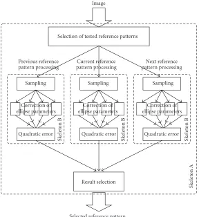
(1) The computations on the previous, current, and next reference patterns can be done independently and in parallel (seeSection 3.2for details about reference pat-terns). These computations are independent and in-volve a similar workload. The first parallelisation level, therefore, matches a first data-parallel skeleton (skele-ton A inFigure 22). This skeleton will be used to carry out the comparison of all the reference patterns in par-allel.
(2) The matrix multiplication step involved in the pro-cessing of each reference pattern can be further par-allelised. This second parallelisation level matches another nested data-parallel skeleton (skeleton B in Figure 22).
It is important to realise that these two parallelisation lev-els cannot be merged into a single one because the three in-ner matrix multiplications cannot be merged into a single matrix multiplication. More precisely, three different inter-action matrices (namedAin the previous section) and three different gray-level vectors (namedVdiff) have to be con-sidered. For each reference pattern, only one vector must be multiplied by one matrix. So merging the three matrices into a single one and the three vectors into a single one will not only result in extra computing time but will also produce er-roneous results.
At both levels, the data-parallel computations are very regular (i.e., they process data sets whose size is known at compile time and their complexity does not depend on the values of these data). This makes them perfect candidates for an implementation with a SCM skeleton. The parallel struc-ture of the application is therefore made up of two nested SCM skeletons, the inner SCM skeleton playing the role of thecomputefunction for the outer skeleton.
Image
Selection of tested reference patterns
Previous reference pattern processing
Current reference pattern processing
Next reference pattern processing
Sampling Sampling Sampling
Correction of ellipse parameters
Correction of ellipse parameters
Correction of ellipse parameters
Quadratic error Quadratic error Quadratic error
Sk
elet
o
n
B
Sk
elet
o
n
B
Sk
elet
o
n
B
Sk
elet
o
n
A
Result selection
Selected reference pattern
and real position of the tracked pattern in the image
Figure22: General parallel structure.
4.2. Implementation
Once the parallel structure of the application has been iden-tified, the SKiPPER-II environment can be used to obtain a parallel implementation. From a programmer’s point of view, this involves
(1) expressing this parallel structure using some kind of description language (i.e., specifying which skeletons are used and in what order),
(2) providing the application-specific sequential functions to be used as arguments to the skeletons.
In previous SKiPPER versions, expressing the parallel struc-ture was carried out using a subset of the Caml language [4]. The same approach is intended to be used for SKiPPER-II. In this case, the intermediate description of the application (as a tree of TF/II skeletons) will be generated by a modified version of the Camlflow tool [19]. In the current version of SKiPPER-II, this step is still handled manually, that is, the intermediate description is provided by the programmer in the form of a C descriptor which can be used directly by the kernel. This descriptor encodes, in the form of a C array, the tree of TF/II skeletons that matches the skeletal structure of the application. For the tracker application, the
correspond-#define SKL NBR 2
SK2 Desc app desc [SKL NBR]=
{
{SKO, END OF APP, MASTER, SK1},
{SK1, UPPER, SLAVE, NIL}
};
Algorithm4: Encoding the parallel structure of the tracker appli-cation. C encoding for SKiPPER-II.
ing descriptor5is given inAlgorithm 4(Figure 23recalls the
skeletal structure of the application). There is one line per skeleton. On each line,
(i) the first column is the skeleton ID (for reference), (ii) the second column indicates the skeleton
“continua-tion,” that is, whether its results must be sent to an up-per level or to another skeleton at the same level,6
(iii) the third column tells whether this skeleton acts as a slave (i.e., is nested) or as a master,
S1
S2
F2
M2
M1
F2 F2 F2 F2 F2 F2 F2 F2 F2 F2 F2
S2 S2
M2 M2
Original application using SCM skeletons
Inner
SCM
sk
elet
on
(sk
elet
o
n
B
)
Out
er
SCM
sk
elet
on
(sk
elet
o
n
A
)
S1 M1
S2
M2 S2M2 S2M2
F2 F2 F2 F2 F2 F2 F2 F2 F2 F2 F2 F2
Internal TF/II tree corresponding to the intermediate description
Support process User sequential function
Inner
T
F/II
sk
elet
on
(sk
elet
o
n
B
)
Out
er
T
F/II
sk
elet
on
(sk
elet
o
n
A
)
S1: Selection of tested reference patterns S2: Sampling
M1: Result selection
F2: Correction of ellipse parameters M2: Quadratic error
Figure23: Encoding the parallel structure of the tracker application. Graphical representation.
(iv) the last column gives the ID of the destination skele-ton.
The second step in using SKiPPER-II is providing the application-specific sequential functions. These functions— to be used as arguments to the specified skeletons—are writ-ten in C and must be “pure” functions (no side-effect, no reference to global variables or shared data). All nonatomic arguments7must be passed by address and all results must be
returned by address. The prototypes of the sequential func-tions for the tracker application are given inAlgorithm 5.
In the current implementation of SKiPPER-II, the pro-grammer is also required to write a few lines of stub code to allow the application-specific sequential functions to be linked with the kernel code. The main role of this stub code is to alleviate the lack of support for data polymorphism in the C language (at the kernel level, all application-specific functions must have a uniform interface, in which all argu-ments and results are passed/returned as untyped buffers). This stub code is very systematic and repetitive (it essentially
7Byatomicarguments, we mean those having nonstructured data types, such as int, float, and so forth.
consists in packing/unpacking application-level data struc-tures into/from kernel-level (char ) arrays) and could be automated.
5. RESULTS AND DISCUSSION
The benchmark was performed on Intel Celeron Beowulf machine (32×533 MHz nodes, 100 Mbps switched Ethernet network). Figures24and25, respectively, show the comple-tion time of the algorithm and the relative speedup obtained in increasing the number of nodes for two quantities of sam-pled points in the elliptic area (170 and 373 sample points).
It must be noticed that using more than 170 sample is not giving better results in terms of tracking capabilities (using 170 points already provides a sufficiently robust tracking). This number was increased in order to further assess the per-formances of SKiPPER-II kernel, since it directly influences the computation/communication ratio.
The curves in Figures 24 and 25 exhibit three phases which can be related to the behaviour of the SKiPPER-II ker-nel.
S1(
int pattern number, /I /
Ellipse current ellipse, /I/O/
int tracker number to test / O/
); S2(
Ellipse current ellipse, /I/O/
int tracker number to test, /I/O/
int gray level vector size, / O/
float gray level difference-vector, / O/
int matrix line number, / O/
float matrix / O/
); F2(
Ellipse current ellipse, /I/O/
int tracker number to test, /I/O/
int gray level vector size, /I /
float gray level difference-vector, /I /
int matrix line number, /I/O/
float matrix, /I /
float correction / O/
); M2(
Ellipse current ellipse, /I /
int tracker number to test, /I/O/
int matrix line number, /I /
float correction /I /
float quadratic error, / O/
Ellipse corrected ellipse, / O/
); M1(
Ellipse current ellipse, /I /
int tracker number to test, /I /
float quadratic error, /I /
Ellipse final current ellipse, / O/
int final pattern number / O/
);
Algorithm5: Signature of the application-specific sequential func-tions for the tracker application.
completion time is higher in the multiprocessor case. This negative speedup can be explained by the way the outer SCM skeleton is deployed on the network. In fact, with the run-time mechanism presented inSection 2.4, using two nodes does not provide more computing power but only creates communications. This is because one of the nodes is used as a dispatching process and is not performing useful com-putation at all. When the comcom-putation versus communi-cation is small (as in the 170 points case), this effect can even be observed with 3 nodes because the time to com-municate data to the two nodes doing computations de-stroys the potential gains of performing theses computations is parallel.
55 50 45 40 35 30 25 20 15 10 5 0
1 3 5 7 9 11 13 15 17 19 21 23 25 Number of nodes
C
o
mpletio
n
time
(ms)
170 sampled points 373 sampled points
Figure24: Completion time for 170 and 373 sampled points for 3D face-tracking algorithm parallelisation on an Intel Celeron Beowulf machine.
25
20
15
10
5
0
1 3 5 7 9 11 13 15 17 19 21 23 25 Number of nodes
Speed
up
Linear
170 sampled points 373 sampled points
Figure25: Speedup for 170 and 373 sampled points for 3D face-tracking algorithm parallelisation on an Intel Celeron Beowulf ma-chine.
From 4 to 19 nodes, performance increases with the number of nodes (though not linearly). This phase corre-sponds to the deployment of the inner SCM skeleton, which performs the vector-matrix multiplications in parallel.
nodes matches this fixed parallelism degree.8When the
num-ber of available nodes is higher (19–32), no further paral-lelism can be exploited and hence efficiency decreases. When the number is smaller (4–18), the kernel sequentialises some processings on some nodes (thus providing a form of “virtu-alisation” mechanism).
The relatively poor results in terms of efficiency can be more generally explained by the relatively small computa-tion versus communicacomputa-tion ratio of the parallel version. As a matter of fact, the sequential version of the algorithm was already very efficient because of very few intensive comput-ing stages. This is especially true for the inner parallelisation level because the matrix multiplication is only a (p×N) ma-trix multiplied by the gray-level vector of sizeN.
6. CONCLUSION
This paper presents a skeleton-based parallel programming environment supporting skeleton nesting and the paralleli-sation of a realistic image processing application using this latest capability. As far as we know, the work described here is one of the few reported experiments showing the applica-tion of skeleton nesting facilities for the parallelisaapplica-tion of a realistic application, especially in the area of image process-ing. Indeed the 3D face-tracking algorithm cannot be entirely parallelised without this kind of skeleton combination. This is due to the fact that the different parallelisation levels can-not be merged into a single one and have to be handled by separate nested skeletons.
However, this work also shows that the run-time mech-anism used in SKiPPER-II entails a significant performance penalty, especially when the computation versus communi-cation ratio is low. In this case, skeleton nesting is not a trans-parent operation in terms of efficiency.
As for methodological aspects, we noticed that the par-allelisation of the tracking algorithm only required three to four working days. This time was mainly dedicated to se-lect the right parallelisation structure (which skeletons and how are they connected), and subsequently to split the orig-inal algorithm into computing functions to plug into the skeletons (the original user’s functions have to be splited and their interface rewritten). Concerning parallelisation choices for the 3D face-tracking algorithm, we think that after this experiment, it could be interesting to parallelise the first stage of the algorithm, although it is normally an “off-line” stage. The reason is that decreasing the completion time will bring the opportunity to use all of the processing stages in an “on-line” way in order to use the tracking algorithm for multitarget tracking purposes, like multivehicle track-ing [20]. In this case, speedtrack-ing up this stage could allow the application to learn reference patterns of vehicles on the fly and hence allow it to adapt itself to the road environ-ment without relying on a large prebuilt database of pat-terns.
8For the outer SCM skeleton, the optimal number of nodes is 4 (3 for computing, one for dispatching); for the inner one, this number is 5 (4 + 1).
ACKNOWLEDGMENTS
The authors would like to acknowledge the support of the European Commission through Grant number HPRI-1999-CT-00026 (the TRACS Programme at EPCC, Scotland) and to thank the staffmembers of the Department of Comput-ing and Electrical EngineerComput-ing, the Heriot-Watt University, Edinburgh, Scotland. The authors would also like to thank Santosh Anand, a Graduate from IIT Kampur, India, for his careful review of the paper’s English.
REFERENCES
[1] D. Ginhac, J. S´erot, and J.-P. D´erutin, “Fast prototyping of image processing applications using functional skeletons on
MIMD-DM architecture,” inIAPR Workshop on Machine
Vi-sion Applications, pp. 468–471, Chiba, Japan, November 1998.
[2] D. Ginhac, Prototypage rapide d’applications parall`eles de
vi-sion artificielle par squelettes fonctionnels, Ph.D. thesis, Univer-sit´e Blaise-Pascal, Clermont-Ferrand, France, January 1999. [3] J. S´erot, D. Ginhac, and J.-P. D´erutin, “Skipper: a
skeleton-based parallel programming environment for real-time
im-age processing applications,” in5th International Conference
on Parallel Computing Technologies (PACT ’99), V. Malyshkin,
Ed., vol. 1662 ofLecture Notes in Computer Science, pp. 296–
305, Springer-Verlag, Petersburg, Russia, September 1999. [4] J. S´erot, D. Ginhac, R. Chapuis, and J.-P. D´erutin, “Fast
pro-totyping of parallel-vision applications using functional
skele-tons,”Machine Vision and Applications, vol. 12, no. 6, pp. 271–
290, 2001.
[5] R. Coudarcher, J. S´erot, and J.-P. D´erutin, “Implementation of a skeleton-based parallel programming environment
sup-porting arbitrary nesting,” in6th International Workshop on
High-Level Parallel Programming Models and Supportive Envi-ronments (HIPS’01), F. Mueller, Ed., vol. 2026 ofLecture Notes in Computer Science, pp. 71–85, Springer-Verlag, San Fran-cisco, Calif, USA, April 2001.
[6] M. Hamdan, G. Michaelson, and P. King, “A scheme for
nest-ing algorithmic skeletons,” inProc. 10th International
Work-shop on Implementation of Functional Languages (IFL ’98), C. Clack, T. Davie, and K. Hammond, Eds., pp. 195–212, Lon-don, UK, September 1998.
[7] G. Michaelson, N. Scaife, P. Bristow, and P. King, “Nested
al-gorithmic skeletons from higher order functions,”Parallel
Al-gorithms and Applications, vol. 16, no. 2-3, pp. 181–206, 2001, Special issue on high level models and languages for parallel processing.
[8] M. Hamdan, A Combinational framework for parallel
pro-gramming using algorithmic skeletons, Ph.D. thesis, Heriot-Watt University, Department of Computing and Electrical Engineering, Edinburgh, UK, January 2000.
[9] F. Jurie and M. Dhome, “A simple and efficient template
matching algorithm,” inProc. 8th IEEE International
Con-ference on Computer Vision (ICCV ’01), vol. 2, pp. 544–549, Vancouver, BC, Canada, July 2001.
[10] M. Cole,Algorithmic Skeletons: Structured Management of
Par-allel Computation, Pitman/MIT Press, London, UK, 1989.
[11] M. Cole, “Algorithmic skeletons,” inResearch Directions
in Parallel Functional Programming, K. Hammond and G. Michaelson, Eds., pp. 289–303, Springer, UK, November 1999.
[12] J. S´erot, “Embodying parallel functional skeletons: an
exper-imental implementation on top of MPI,” in3rd Intl Euro-Par
[13] N. Scaife, A dual source parallel architecture for computer
vi-sion, Ph.D. thesis, Heriot-Watt University, Department of
Computing and Electrical Engineering, Edinburgh, UK, May 2000.
[14] T. Grandpierre, C. Lavarenne, and Y. Sorel, “Optimized rapid prototyping for real-time embedded heterogeneous
multipro-cessors,” inProc. IEEE 7th International Workshop on
Hard-ware/Software Codesign (CODES ’99), pp. 74–79, Rome, Italy, May 1999.
[15] W. Gropp, E. Lusk, N. Doss, and A. Skjellum, “A
high-performance, portable implementation of the MPI message
passing interface standard,”Parallel Computing, vol. 22, no. 6,
pp. 789–828, 1996.
[16] R. Coudarcher, Composition de squelettes algorithmiques:
ap-plication au prototypage rapide d’apap-plications de vision, Ph.D. thesis, LASMEA, Blaise-Pascal University, Clermont-Ferrand, France, December 2002.
[17] G. D. Hager and P. N. Belhumeur, “Efficient region tracking
with parametric models of geometry and illumination,”IEEE
Trans. Pattern Anal. Machine Intell., vol. 20, no. 10, pp. 1025– 1039, 1998.
[18] F. Dellaert and R. Collins, “Fast image-based tracking by
se-lective pixel integration,” inInternational Conference on
Com-puter Vision Workshop on Frame-Rate Vision, Corfu, Greece, September 1999.
[19] J. S´erot, “Camlflow: a caml to data-flow translator,” inTrends
in Functional Programming. Volume 2, S. Gilmore, Ed., pp. 129–141, Intellect Books, Bristol, UK, 2001.
[20] F. Marmoiton, F. Collange, P. Martinet, and J.-P. D´erutin, “A
real time car tracker,” inProc. International Conference on
Ad-vances in Vehicle Control and Safety (AVCS ’98), pp. 282–287, Amiens, France, July 1998.
R´emi Coudarcheris a computer science engineer. He graduated from ISIMA, France, and received his Ph.D. degree in computer science from Blaise-Pascal University, France. He has been a post-doc fellow at INRIA, France. His research interests include parallel image processing, and methodologies for parallel and distributed programming and grid computing.
Florent Ducultyis an engineer in electrical science. He graduated from CUST, France, and has a Ph.D. degree in computer science from Blaise-Pascal University, France. His research interests include image processing applied to robotics motion by visual servoing.
Jocelyn Serotis an Associate Professor in electrical engineering at Blaise-Pascal University, France. His research interests are in the de-velopment and use of methodologies for parallel programming, es-pecially in the field of image processing.
Fr´ed´eric Jurieis a Researcher at CNRS, France. His researches are concerned with image processing, especially movement and object detection, and image recognition from appearance.
Jean-Pierre Derutinis a Full Professor in electrical engineering at Blaise-Pascal University, France. His research interests are in the de-sign of dedicated and embedded parallel computers for real-time image processing.
![Figure 15: Completion time for the divide-and-conquer bench-mark (SKiPPER-I) (extract of [2]).](https://thumb-us.123doks.com/thumbv2/123dok_us/1137451.1142668/11.600.57.286.73.239/figure-completion-time-divide-conquer-bench-skipper-extract.webp)