An imaging algorithm based on keystone transform for one-stationary bistatic SAR of spotlight mode

R E S E A R C H

Open Access

An imaging algorithm based on keystone

transform for one-stationary bistatic SAR of

spotlight mode

Xiaolan Qiu

, Florian Behner

, Simon Reuter

, Holger Nies

, Otmar Loffeld

, Lijia Huang

, Donghui Hu

and Chibiao Ding

Abstract

This article proposes an imaging algorithm based on Keystone Transform for bistatic SAR with a stationary receiver. It can efficiently be applied to high-resolution spotlight mode, and can directly be process the bistatic SAR data which have been ranged compressed by the synchronization reference pulses. Both simulation and experimental results validate the good performance of this algorithm.

Keywords:Bistatic SAR, Imaging algorithm, Keystone transform

Introduction

Bistatic SAR is more flexible in data acquisition geom-etry compared with traditional monostatic SAR. How-ever, this flexibility is gained at the cost of increasing system complexity, which not only refers to increasing hardware system complexity due to synchronization needs of transmitter and receiver, but also refers to increas-ing processincreas-ing complexity. As for the synchronization, the easy to realize and commonly used strategy is using an additional antenna to receive the direct pulses from trans-mitter, and then using these directly received pulses as a reference for range compression. As for bistatic SAR im-aging, a number of studies have been done and several kinds of imaging algorithms have been proposed for dif-ferent configurations [1-9]. Furthermore, a number of bistatic SAR experiments with different configurations [10-15] have successfully been carried out till now.

Among the various configurations of bistatic SAR, the so-called one-stationary configuration, which is usually formed by an existing moving transmitter (i.e., space-borne SAR, airspace-borne SAR, or even navigation satellite [16]) and a stationary passive receiver, is, in the authors’ opinion, one of the most practical configurations. On

the one hand, it is inexpensive to build, and on the other hand, it can easily be extended to multi-receiver stations and then obtain multi-baseline interferometric SAR images to rebuild accurate DEM of regions of interest.

The main difficulty of imaging processing for the one-stationary bistatic configuration has been pointed out and solved to some extent in the authors’previous pub-lication [17,18]. However, the former algorithm mainly aims at the stripmap mode and may not be suitable for the high-resolution spotlight mode. In spotlight mode, the pulse repetition frequency (PRF) is usually smaller than the Doppler bandwidth of a single target. So, the dechirp method is commonly used for efficient proces-sing. Meanwhile, if range compression is done by the directly received pulses from the synchronization chan-nel, the dechirp in azimuth has already been done within this range compressing step. After this dechirp step, the residual range and phase histories are still range– azimuth variant, while the linear term is predominant. In the high-resolution case, the range histories are bend-ing more severely as the range bins are smaller. Hence, the differential range histories for those targets with the same bistatic range will exceed one range gate; therefore, the precondition of the NLCS algorithm based on azi-muth perturbation in [18] is no longer valid. Till now, almost all the published images of the one-stationary bistatic SAR experiments have been focused by the uni-versal back-projection (BP) algorithm [10,16]. Although

* Correspondence:[email protected]

1_{Institute of Electronics, Chinese Academy of Sciences, Beijing 100190, China} 2

Key Laboratory of Spatial Information Processing and Applied System, Chinese Academy of Sciences, Beijing 100190, China

Full list of author information is available at the end of the article

good quality images can be obtained using this algo-rithm, the main shortcoming is its computational ineffi-ciency. The computation load of BP algorithm for producing an image, whose size is M * M and the synthetic aperture length isK, is on the order ofM*M*K (i.e., O(M*M*K)). This can be very large for a big size high-resolution image.

In this article, an efficient imaging algorithm based on the Keystone Transform for one-stationary bistatic SAR, whose computation load is on the order of M2log2M, is proposed. The Keystone Transform is usually used in ISAR processing. The idea of using this transform to correct the azimuth variant range cell migration (RCM) in medium-earth–orbit SAR imaging has been proposed in the authors’ another article (H Lijia, Q Xiaolan, H Donghui, D Chibiao, A novel algorithm based on keystone transform and azi-muth perturbation for medium-earth-orbit SAR, submit-ted). In this study, we propose to use the Keystone Transform for bistatic SAR imaging. The approach can dir-ectly be performed on bistatic SAR data which has been range compressed by the synchronization reference pulses, which makes it convenient to use. The experimental data of the HITCHHIKER system at University of Siegen/ZESS is used to test this algorithm, and good bistatic SAR images are obtained by this algorithm.

This article is organized as follows:“Geometry and signal model” section describes the one-stationary bistatic SAR geometry, and builds the signal model;“Imaging algorithm based on Keystone Transform”section introduces the pro-posed imaging algorithm step-by-step and shows the block diagram of the algorithm; “ Simulation and experimental results” section validates the imaging algorithm through simulations and experimental results, and “Conclusion” section concludes the article.

Geometry and signal model One-stationary bistatic SAR geometry

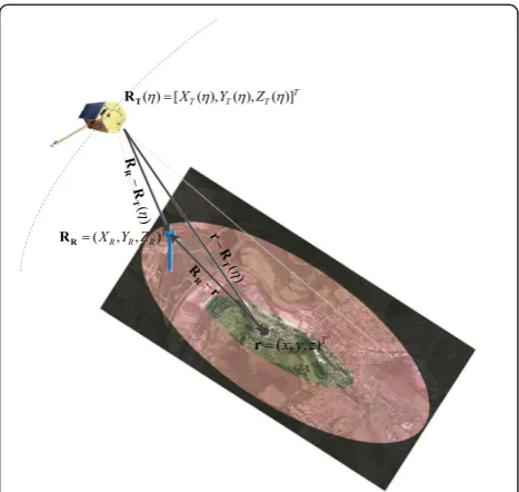
The one-stationary bistatic SAR geometry is illustrated in Figure 1. In some Earth-fixed coordinates, the vector of stationary receiver location is RR= (XR,YR,ZR)T. The vector of the moving transmitter is RT(η) = [XT(η),YT(η), ZT(η)]T, when the azimuth time (slow time) isη. An arbi-trary point scatter on the earth is denoted asr= (x,y,z)T.

Signal model

If the time when the received echo reaches the max-imum power is considered asη= 0, the range history of the direct pulses and that of the target r in spotlight mode can be, respectively, represented as follows.

RDð Þ ¼η jRRRTð Þηj ð1Þ

Rbiðη;rÞ ¼jrRTð Þη j þjrRRj ð2Þ

If the nominal frequency of the transmitted signal is f0Tand the transmitted signal has a rectangular envelope with a time duration T and a wide bandwidth, the received signal in direct channel and echo channel be-fore down conversion at timeη+τcan be written as fol-lows, respectively,

gDðη;τÞ≈wDðη;τÞrect τ

RDð Þη =c

T

p½τRDð Þη=c

:expj2πf0T½ηþτRDð Þη=c

þjφT½ηþτRDð Þη =c

ð3Þ

gðη;τÞ≈∫∫

x;y

wðη;τ;rÞσð Þr rect τRbiðη;rÞ=c T

:p½τRbiðη;rÞ=c

:expfj2πf0T½ηþτRbiðη;rÞ=cg

:expfjφ_T½ηþτRbiðη;rÞ=cg

8 > > > > < > > > > :

9 > > > > = > > > > ;

dxdy

ð4Þ

wherep(τ) represents the transmitted waveform;τ repre-sents the fast time (range time), whose origin is when the pulse is transmitted; φT is the phase error of the transmitter oscillator;σ(r) is the scattering coefficient of target r; wD(η,τ) and w(η,τ;r) mean the weight due to the transmitter and receiver antenna pattern, propaga-tion loss, etc. Without loss of generality, w(η,τ;r) and wD(η,τ) are considered as constants here and are ignored in the following analysis.

The approximate equal marks in Equations (3) and (4) come from neglecting the variation ofRDandRbiwithτ, respectively.

If the nominal frequency of the receiver is f0R, the down conversion signal atη+τis then

gRðηþτÞ ¼ expfj2πf0RðηþτÞ jφRðηþτÞg ð5Þ

whereφRis the phase error of the receiver oscillator. Hence, after down conversion, the direct channel signal is

sDðη;τÞ ¼ rect τ

RDð Þη=c

T

p½τRDð Þη=c

:expfj2πf0TRDð Þη =cg

:expfj2πðf0Tf0RÞðηþτÞg

:expfjφ_T½ηþτRDð Þη=c jφRðηþτÞg

ð6Þ

and the echo channel signal is

sðη;τÞ ¼ ∫∫

x;y

σð Þr rect τRbiðη;rÞ=c T

p

τRbiðη;rÞ

c

:expfj2πf0TRbiðη;rÞ=cg

:expfj2πðf0Tf0RÞðηþτÞg

:expjφ_T½ηþτRbið Þη =c

jφRðηþτÞg

8 > > > > > > > > > > > < > > > > > > > > > > > : 9 > > > > > > > > > > > = > > > > > > > > > > > ; dxdy ð7Þ

Compress s(η,τ) in range direction using sD(η,τ), which is

s1ðη;τÞ ¼IFFTτ

shiftFFTτ½sðη;τÞ :conj FFTf τ½sDðη;τÞg

ð8Þ

Here, shift means to shift the spectrum which is cen-tered atf0T−f0Rto be centered at zero in the range fre-quency domain and conj means conjugation. Then we have

s1ðη;τÞ≈ ∫∫ x;y

σð Þr sinc τRbiðη;rÞ RDð Þη c

:expfj2πf0T½Rbiðη;rÞ RDð Þη =cg 8 < : 9 = ;dxdy ð9Þ

The approximation in the above equation comes from

omitting of the phase difference between rect τRDð Þη=c

T

h i

expfjφ_RðηþτÞgand rect τRbiðη;rÞ=c

T

h i

expfjφ_RðηþτÞg, which can usually be ignored.

It can be seen from Equation (9) that, after range com-pression using the reference signal from the direct chan-nel, the time synchronization problem is solved because

all the received echo pulses are aligned to the knownRD (η). The frequency synchronization problem is solved because the direct and the echo pulses are generated by the same transmitter. The phase synchronization is also solved as long as no additional phase differ-ence is introduced by the two receive channels. This is because the phase errors caused by the transmitter are the same in direct and echo pulses and hence can be counteracted; besides, as the direct and the echo pulses are received with small time difference, the phase errors caused by the receiver in direct and in echo pulses are nearly the same and also can be counteracted. So, as has been said in the introduc-tion, this is the easiest and commonly used synchronization method. Therefore, it is reasonable to start bistatic SAR focusing from s1(η,τ).

The residual range history after range compression is

Rbicðη;rÞ ¼Rbiðη;rÞ RDð Þη ð10Þ

It can be seen that, if the receiver is near the scenario, the higher order terms inRbic(η;r) will be much smaller than those in the original range history Rbi(η;r), so the Doppler bandwidth of the targets after range compres-sion by the reference pulses is much smaller than the original Doppler bandwidth. For example, in the spaceborne-ground bistatic SAR configuration, such as in TerraSAR-X/HITCHHIKER experiment, the original Doppler bandwidth is about 5192 Hz, but after the range compression using the direct pulses, the residual Dop-pler bandwidth shrinks to be about 62 Hz. Therefore, if traditional imaging algorithms, which correct RCM in the azimuth frequency domain, are applied, a Doppler wideband signal rebuilding step should be adopted, which makes them not very convenient to use. In the next section, an algorithm based on the Keystone Trans-form which does not need Doppler signal rebuilding will be introduced.

Imaging algorithm based on Keystone Transform Keystone Transform for linear RCM correction

In one-stationary spotlight bistatic SAR cases, such as spaceborne-ground cases and straight path airborne-ground cases, the residual range history can be approxi-mated as follows:

Rbicðη;rÞ≈Rbicð0;rÞ þAηþBη2þCη3þDη4 ð11Þ

transmitter flies alongy-axis with a constant velocityVT, then the parametersAandBare as follows

Að Þ ¼r VT

YTð Þ 0 y rRTð Þ0

j j

YTð Þ 0 YR RRRTð Þ0

j j

ð12Þ

Bð Þ ¼r VT2

cos2_θ Tð Þr rRTð Þ0

j j

cos2_θ Tð ÞRR RRRTð Þ0

j j

ð13Þ

where

θTð Þ ¼r cos1

ffiffiffiffiffiffiffiffiffiffiffiffiffiffiffiffiffiffiffiffiffiffiffiffiffiffiffiffiffiffiffiffiffiffiffiffiffiffiffiffiffiffiffiffiffiffiffiffiffiffiffiffiffiffiffi XTð Þ 0 x

½ 2_þ

ZTð Þ 0 z

½ 2

q

rRTð Þ0

j j 8 < : 9 = ; ð14Þ

θTð Þ ¼RR cos1

ffiffiffiffiffiffiffiffiffiffiffiffiffiffiffiffiffiffiffiffiffiffiffiffiffiffiffiffiffiffiffiffiffiffiffiffiffiffiffiffiffiffiffiffiffiffiffiffiffiffiffiffiffiffiffiffiffiffiffiffiffi XTð Þ 0 XR

½ 2_þ

ZTð Þ 0 ZR

½ 2

q

RRRTð Þ0

j j 8 < : 9 = ; ð15Þ It can be seen that A(r) nearly linearly depends on y, which means it is strongly azimuth variant, while B(r) depends on |r−RT(0)| and θT(r), which is more slightly azimuth variant than A(r). The higher-order terms are much smaller than the first two-order terms, so here we pay more attention toA(r) andB(r).

In case of a complex trajectory, these parameters can nu-merically be obtained by polynomial fit to the residual range history.

After performing a range Fourier transform ons1(η,τ), we have

S1ðη;fÞ ¼ ∫∫

x;yσð Þr exp j2π

f0Tþf

c Rbicðη;rÞ

dxdy

≈ ∫∫

x;y

σð Þr exp j2πf0Tþf

c Rbicð0;rÞ

:exp j2πf0Tþf

c AηþBη

2_þCη3_þDη4

8 > > < > > : 9 > > = > > ;dxdy ð16Þ The Keystone Transform for linear decoupling is as follows. Let

ξ¼f0Tþf

f0T η ð17Þ

then

S1ðξ;fÞ≈ ∫∫

x;y

σð Þr:exp j2πf0Tþf c Rbicð0;rÞ

:exp j2π λ Aξ

exp j2π λ

f0T

f0Tþf

Bξ2

:exp j2π λ

f0T

f0Tþf

2

Cξ3

( )

:exp j2π λ

f0T

f0Tþf

3

Dξ4

( ) 8 > > > > > > > > > > > > > < > > > > > > > > > > > > > : 9 > > > > > > > > > > > > > = > > > > > > > > > > > > > ; dxdy ð18Þ

whereλ=c/f0T.

In the general SAR case, |f| << f0T, so the following approximation can be applied.

f0T

f0Tþf≈

1 f f0T

þ f

f0T 2

f

f0T 3

ð19Þ

f0T

f0Tþf

2

≈12 f f0T

þ3 f f0T

2

4 f

f0T 3

ð20Þ

f0T

f0Tþf

3

≈13 f f0T

þ6 f f0T

2

10 f

f0T 3

ð21Þ

Substituting Equations (19)–(21) into Equation (18) and reorganizing yields

S1ðξ;fÞ≈ ∫∫ x;y

σð Þr exp j2π λ

f0Tþf

f0T

Rbicð0;rÞ

:expfjψ_Aðξ;rÞg :exp jψcoupðξ;f;rÞ

n o 8 > > > < > > > : 9 > > > = > > > ; dxdy ð22Þ where

ψAðξ;rÞ ¼

2π

λ AξþBξ2þCξ3þDξ4

ð23Þ

is the azimuth phase which only depends onξ. And

ψcoupðξ;f;rÞ ¼

2π λ

f f0T

Bξ2

2Cξ33Dξ4

þ2π λ

f f0T

2

Bξ2þ3Cξ3þ6Dξ4

þ2π λ

f f0T

3

Bξ2

4Cξ310Dξ4

ð24Þ

is the phase containing the azimuth–range coupling. It can be seen from this phase that no linear coupling be-tween fandξ exists, which means that the linear RCMs for all targets have been corrected by the Keystone Transform. Then, a bulk phase compensation according to the reference target can be done by the following function

H_compðξ;fÞ ¼ exp j2π

λ

f f0T

B_refξ2þ2Crefξ3þ3Drefξ4

:exp j2π

λ

f f0T

2

Brefξ2þ3Crefξ3þ6Drefξ4

( )

:exp j2π

λ

f f0T

3

B_refξ2_þ4C

refξ3þ10Drefξ4

( )

ð25Þ

where subscript ref means the value calculated at the reference position (usually to be the scene center). Here, we denoteS2(ξ,f) =S1(ξ,f)Hcomp(ξ,f).

higher-order terms of f/f0T in the remaining coupled phase will decrease the range focusing quality. Usually, if the quadratic phase error is smaller than π/4, the im-aging quality is acceptable. So, the following condition is used to restrict the processing area.

max (

2π λ

fB

2f0T

2

½Bð Þ r Brefξ2þ3½Cð Þ r Crefξ2

þ6½Dð Þ r Drefξ2 )

≤π

4 ð26Þ

This ensures that in each processing area, all targetsr at eachξhave quadratic phase error that smaller thanπ/ 4, so the imaging quality is guaranteed.

Residual RCM correction

If the higher-order term phases ofS2(ξ,f) are restricted and their effects can be neglected. Then, applying an

inverse Fourier transform to S2(ξ,f), the signal in the time domain is

s2ðξ;τÞ≈ ∫∫ x;y

σð Þr exp j2π

λ Rbicð0;rÞ

:sinc τRbicð0;rÞ R r RCMðξ;rÞ c

:expfjψ_Aðξ;rÞg 8

> > > > < > > > > :

9 > > > > = > > > > ;

dxdy

ð27Þ

where

Rr_RCMðξ;rÞ ¼ðBBrefÞξ2þ2ðCCrefÞξ3

þ3ðDDrefÞξ4 ð28Þ

It can be seen that the position of a target in the image plane along the fast time axis is determined byRbic(0;r), and the residual RCM is a function of the target loca-tion, which is range–azimuth variant. Usually, the RCM, which is within half a slant range resolution cellρr, can

be neglected in SAR imaging field. So, if the following restriction

maxRr_RCMðξ;rÞ<ρr

2 ð29Þ

is satisfied for any r, then residual RCM correction step can be omitted. If this cannot be satisfied for the whole scene, then the sub-swath strategy can be

used to deal with the azimuth variance and

interpolation in two-dimensional time domain can correct the range variance of RRCMr (ξ;ri).

The sub-swath dealing with the azimuth variance is as follows. First, a reference position r_i is chosen for each range gate i (usually choose to be in the middle of azimuth swath). Then, the azimuth proces-sing sub-swath is restricted according to the follow-ing condition

maxRr_RCMðξ;rÞ R_RCMr ðξ;riÞ<ρr=2 ð30Þ

Consider the main component (i.e., the second-order term) in |RRCMr (ξ;r)−RRCMr (ξ;ri)| and calculate the above restriction, we have

max Rr

RCMðξ;rÞ RrRCMðξ;riÞ

≈max VT2ξ2

cos2_θ Tð Þr rRTð Þ0

j j

cos2_θ Tð Þri riRTð Þ0

j j

≈max VT

2_ξ2

riRTð Þ0

j jcos2θTð Þ r cos2θTð Þri

<ρr

2 ð31Þ It can be seen that the azimuth sub-swath can be restricted through θT(r), and the limitation of θT(r) is variant with range.

Azimuth compression

After the above steps, the final azimuth compression step can be done. The higher-order term of ψA(ξ;r), which is

ψh Aðξ;rÞ ¼

2π

λ Bξ2þCξ3þDξ4

ð32Þ

is desired to be removed for fine focusing. If the azimuth variation ofψAh(ξ;r) is smaller thanπ/4, then for each range gate, the following phase compensation filter is applied

HAcðξ;riÞ ¼ exp j2_λπBð Þri ξ2þCð Þri ξ3þDð Þri ξ4

ð33Þ

Then the final focused image can be obtained through azimuth Fourier transform. The final image can be written as

s3ðfξ;τÞ ¼∫∫

x;y

σð Þr exp j2π

λ Rbicð0;rÞ

:sinc τRbicð0;rÞ

c

:sinc fξþAð Þ_λr

8 > > < > > :

9 > > = > > ;dxdy

ð34Þ Table 1 Transmitter and receiver parameters for

simulation

Symbol Meaning Quantity

f0T Transmitter frequency 9.65 GHz

fB Signal bandwidth 300 MHz

fs Sample rate 330 MHz

PRF PRF 3224.35 Hz

f0R Receiver frequency 9.70 GHz

Ta Data acquisition time 2.48 s

Na Azimuth pulse number 8000

Nr Range sample number 30000

If the azimuth variation ofψAh(ξ;r) is larger thanπ/4, an additional step of sub-segment azimuth processing is needed. This means to cut the above image into several small segments along azimuth direction (according to the azimuth variation of ψAh(ξ;r)), and then to perform an in-verse Fourier transform to get the azimuth time domain signal for each segment. The differential phase betweenψAh (ξ;r) of this segment and the phase of HAc(ξ;r) for each range gate can be calculated through range history, and be compensated for this segment. Finally, all the segments are transformed to the frequency domain and combined to-gether to get the final fine focused image.

Geocoding

As can be seen from Equation (34), the axes of the focused image are τ and fξ, whose limitations are [τ1: 1 /fs:τ1+ (Nr−1) /fs] and [−fPRF/ 2 :fPRF/Na:fPRF/ 2], respectively. Here,Nris the image size in range direction andNais the size in azimuth direction.fs is the sample rate andfPRF is the PRF. τ1 corresponds to the sample delay of the first range gate after range compression. When trigger time of the echo channel is the same as that of the direct pulse channel, thenτ1=RD(0) /c.

The position of targetrin the image plane is as follows

τr¼Rbicð0;rÞ c fξr¼

Að Þr λ

8 > < > :

ð35Þ where

Að Þ ¼r dRbicðη;rÞ dt

_η¼

0

¼VTð Þ0 •½rRTð Þ0

rRTð Þ0

j j

VTð Þ0 •½RRRTð Þ0

RRRTð Þ0

j j

ð36Þ

(a)

(b)

(c)

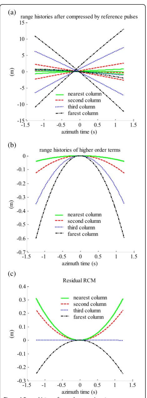
Figure 4Range history after each processing step.

Here, VT is the transmitter velocity vector in the

Earth-fixed coordinates. If a DEM of the scenario is provided, then geocoding can be done according to Equations (1), (2), (10), (35), and (36).

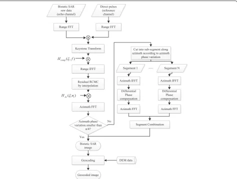
Block diagram of the algorithm

The block diagram of the proposed algorithm for one-stationary bistatic SAR of spotlight-mode is shown in Figure 2. It can be seen that the algorithm is quite effi-cient as only a pair of range Fourier transforms and a single azimuth Fourier transform are needed for the non-severe azimuth variant case.

Simulation and experimental results

To testify this algorithm, both simulated bistatic SAR data and the real experimental data of HITCHHIKER are processed using this algorithm, and results are ana-lyzed and compared in this section.

Point target simulation

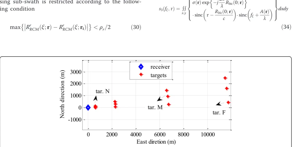
The parameters of point target simulation are according to the TerraSAR-X/HITCHHIKER bistatic experiment in Siegen, Germany. The locations of the stationary re-ceiver and the scene center described by [latitude, longi-tude, height] are [50.910787 deg, 8.027111 deg, 434.91 m] and [50.913650 deg, 8.059843 deg, 292 m], respect-ively. The transmitter and receiver parameters are shown in Table 1 and the locations of simulated targets in East-North-Height coordinates with the receiver as the origin are shown in Figure 3. These targets represent the main scenario area of the real experiment. In order to observe the azimuth variation of the range history, each column of targets has the same bistatic range, so each column of targets are on an ellipse arc.

After the range compressing using reference pulses, the residual range histories (without the constant term) of the simulated targets are shown in Figure 4. It can be seen that the RCMs are different for different targets. From Figure 4a, we can see that, for each column of tar-gets, the liner components of their RCMs are changing with their azimuth location. This is consistent with Equation (12). The residual RCMs after the linear terms have been removed by the Keystone Transform are shown in Figure 4b. It can be seen that the residual RCMs are mainly range variant. The targets within the same column (which have the same bistatic range when η= 0) have almost the same residual RCMs. After the

(a)

(b)

(c)

Figure 6Imaging result of the simulated targets.

Table 2 Interferometry phases of the simulated targets Target Differential phase (degree) Phase error

(degree) Measured from images Ideal value

N 156.9894 157.1157 −0.1263

M −55.1917 −55.0924 −0.0993

bulk residual RCM correction byHcomp, the residual RCMs for the simulated targets are all smaller than 0.35 m (see Figure 4c). This is smaller than half a range resolution cell (a range resolution cell is about 0.886 m here), so the range variant residual RCM correction can be omitted in this case. The residual azimuth phases after azimuth phase compensation for each range gate usingHAc are shown in Figure 5. It can be seen that the azimuth phase errors for all the targets in the scene are smaller than 25°, so the sub-segment processing step is not needed in this simulation. The imaging results are shown in Figure 6. It can be seen that targets at different locations are all well focused.

To testify the phase preserving ability of this algorithm, and to answer the question: whether the image processed by this algorithm is able to do the further interferometry processing, another set of raw data is simulated. All the parameters are the same with the first raw data, except that the receiver’s location described by [latitude, longi-tude, height] is [50.910787 deg, 8.027111 deg, 435.91 m]. The differential phases of target N, M, F are shown in Table 2, from which we can see that the differential phases are very close to the ideal differential phases cal-culated by 2π

λ Rbicð0;rÞ Rnewbicð0;rÞ

, where Rbicnew means the range corresponding to the second receiver. The variance of the differential phase errors of all the simulated targets is 0.0919°. This means that the algo-rithm provided here is well phase preserving and can support the interferometry processing.

Experimental data processing and results

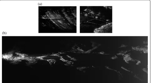
The experimental data of the TerraSAR-X/HITCH-HIKER bistatic SAR experiment is processed by the pro-posed algorithm. The focused image before geocoding of the scenario is shown in Figure 7b, and zoomed patches of the image are shown in Figure 7a, from which we can see that the image is well focused.

The image is then geocoded based on the DEM data of the scenario. Overlay the image on to Google earth, all the buildings and roads match very well with the orthophoto, which validates the correctness of the geo-coding method in “Geocoding” section. The geocoded image by proposed algorithm is compared with the imaging result of BP algorithm in Figure 8. It can be seen that the imaging result of the algorithm provided here can compare beauty with the result of BP algo-rithm. In the imaging results, the buildings are well fo-cused, while the trees are a little blur because the weather is windy while data acquisition. The same size (4096*6000) image processed by the algorithm here using Matlab on a single PC takes about 5 min, while processed by BP algorithm on the same PC takes more than 31 h, which validates the efficiency of this algorithm.

Conclusion

This article proposed an imaging algorithm for the one-stationary bistatic SAR in spotlight mode. The main

(a)

(b)

property of the algorithm is using the Keystone Transform to correct the linear part of the two-dimensional variant RCM. The algorithm can directly be applied to the bistatic SAR data which has been range compressed by the refer-ence pulses; therefore, it is efficient and convenient to use.

Both simulation and experimental data processing results validate the algorithm.

Competing interests

The authors declare that they have no competing interests.

Authors’information

Xiaolan Qiu (M’09) received the B.S. degree in electronic engineering from the University of Science and Technology of China in 2004 and the Ph.D. degree in signal and information processing from the Graduate University of the Chinese Academy of Sciences, Beijing, China, in 2009. Since 2009, she has been working in the Institute of Electronics, Chinese Academy of Sciences (IECAS). From May to October 2011, she was supported by K.C. Wong Education Foundation Hong Kong and being a guest scientist in the Center for Sensorsystems (ZESS), University of Siegen. Her current research interests include mono- and bistatic SAR signal processing, SAR interferometry and geostationary orbit SAR.

Florian Behner received the Dipl.Ing. degree in electrical engineering from the University of Siegen, Siegen, Germany, in 2009. He is a research assistant at the Center for Sensorsystems, University of Siegen, Siegen, Germany since 2009 and member of the MOSES postgraduate programme. His current research interests include radar sensor development, bistatic SAR processing and noise SAR. Mr. Behner is member of the DPG (German Physical Society). Simon Reuter received the Dipl.Ing. degree in electrical engineering from the University of Siegen, Siegen, Germany, in 2009. He is a research assistant at the Center for Sensorsystems, University of Siegen, Siegen, Germany since 2009 and member of the MOSES postgraduate programme. His current research interests include radar sensor development, bistatic SAR processing and noise SAR. Mr. Reuter is member of the VDE Association for Electrical, Electronic and Information Technologies.

Holger Nies(M'10) received the Diploma degree in electrical engineering and the Dr. Eng. degree, from the University of Siegen, Siegen, in 1999 and 2006, respectively.

Since 1999 he is a member of the Center for Sensorsystems (ZESS) at the University of Siegen and a lecturer in the Department of Signal Processing and Communication Theory. Since 2010 he is executive director of the International Postgraduate Programme (IPP) "Multi Sensorics" and of the NRW Research School on Multi-Modal Sensor Systems for Environmental Exploration and Safety (MOSES) at the university of Siegen. He is team leader of the SAR group of the ZESS.

He worked in the project sector“Optimal Signal Processing, Remote Sensing - SAR”of ZESS since 1999. He was involved in some project work for Daimler AG (Stuttgart, Germany) in the field of engine modeling and optimization. He was working in the area of SAR interferometry for the German TerraSAR-X mission. Currently he is leading a BMBF funded project regarding optimal processing of TanDEM-X data. His current research interests include bistatic SAR processing, SAR interferometry and distributed data fusion.

Otmar Loffeld(M’05–SM’06) received the Diploma degree in electrical engineering from the Technical University of Aachen, Aachen, Germany, in 1982 and the Eng. Dr. degree and the“Habilitation”in the field of digital signal processing and estimation theory from the University of Siegen, Siegen, Germany, in 1986 and 1989, respectively.

In 1991, he was appointed as a Professor for digital signal processing and estimation theory at the University of Siegen. Since then, he has given lectures on general communication theory, digital signal processing, stochastic models and estimation theory, and synthetic aperture radar. In 1995, he became a Member of the Center for Sensorsystems (ZESS), which is a central scientific research establishment at the University of Siegen (www. zess.uni-siegen.de), where he has been the Chairman since 2005. In 1999, he became the Principal Investigator (PI) on baseline estimation for the X-band part of the Shuttle Radar Topography Mission, where ZESS contributed to the German Aerospace Center’s baseline calibration algorithms. He is the PI for the interferometric techniques in the German TerraSAR-X mission, and together with Prof. Ender from FGAN, he is one the PIs for a bistatic spaceborne airborne experiment, where TerraSAR-X serves as the bistatic illuminator while FGAN’s PAMIR system mounted on a Transall airplane is used as a bistatic receiver. In 2002, he founded the International Postgraduate Program“Multi Sensorics,”and based on that program, he established the“NRW Research School on Multi Modal Sensor Systems for Environmental Exploration and Safety (www.moses-research.de)”at the University of Siegen as an upgrade of excellence, in 2008. He is the Speaker

(a)

(b)

(c)

Figure 8Comparison of the geocoded image results processed

and the Coordinator of both doctoral degree programs, hosted by ZESS. Furthermore, he is the university’s Scientific Coordinator for

“Multidimensional and Imaging Systems.”He is the author of two textbooks on estimation theory. His current research interests include multisensor data fusion, Kalman filtering techniques for data fusion, optimal filtering and process identification, SAR processing and simulation, SAR interferometry, phase unwrapping, and baseline estimation. A recent field of interest is bistatic SAR processing.

Prof. Loffeld is a member of the Information Technology Society of the Association for Electrical, Electronic and Information Technologies and a senior member of the IEEE/GRSS. He was the recipient of a Scientific Research award from Northrhine-Westphalia (“Bennigsen-Foerder Preis”) for his works on applying Kalman filters to phase estimation problems such as Doppler centroid estimation in SAR, and phase and frequency demodulation. Lijia Huang(M’10) received the B.S. degree in electronic engineering from Beihang University, Beijing, China, in 2006 and the Ph.D. degree in signal processing and information science at the Graduate University of Chinese Academy of Sciences, Beijing, China, in 2011.

Since 2011, she has been working in the Institute of Electronics, Chinese Academy of Sciences (IECAS). Her current research interests include geostationary orbit SAR and SAR interferometry.

Donghui Hu received the B.S. degree from Peking University, Beijing, China, in 1992, and the M.S. degree from the Beijing Institute of Technology, Beijing, in 2001.

He is currently an Associate Research Fellow with the Institute of Electronics, Chinese Academy of Sciences, Beijing.

His main research interests include SAR signal processing, SAR interferometry and SAR calibration.

Chibiao Ding received the B.S. and Ph.D. degrees in electronic engineering from Beihang University, Beijing, China, in 1997.

Since then, he has been working with the Institute of Electronics, Chinese Academy of Sciences, Beijing, where he is currently a Research Fellow and the Vice Director. In 2006, he got the first prize in China's State

Technological Invention Award.

His main research interests include advanced SAR systems, signal processing technology, and information systems.

Acknowledgments

This study was supported in partly by the Special Foundation of President of the Chinese Academy of Sciences, the National Science Foundation of China (No. 61101200), and the authors are gratefully acknowledging the support of K.C. Wong Education Foundation Hong Kong.

Author details

1_{Institute of Electronics, Chinese Academy of Sciences, Beijing 100190, China.} 2

Key Laboratory of Spatial Information Processing and Applied System, Chinese Academy of Sciences, Beijing 100190, China.3_{Center for}

Sensorsystems (ZESS), University of Siegen, Siegen 57076, Germany.

Received: 8 March 2012 Accepted: 2 September 2012 Published: 12 October 2012

References

1. O Loffeld, H Nies, V Peters, S Knedlik, Models and useful relations for bistatic SAR processing. IEEE Trans. Geosci. Remote Sens.42(10), 2031–2038 (2004) 2. R Wang, O Loffeld, YL Neo, H Nies, Z Dai, Extending Loffeld’s bistatic

formula for the general bistatic SAR configuration. IET Radar Sonar Navigat

4(1), 74–84 (2010)

3. JHG Ender, Signal theoretical aspects of bistatic SAR, inProceedings of IGARSS'03, vol. 3, ed. by (Toulouse, France, 2003), pp. 1438–1441 4. Q Xiaolan, H Donghui, D Chibiao, An Omega-K algorithm with phase error

compensation for bistatic SAR of a translational invariant case. IEEE Trans. Geosci. Remote Sens.46(8), 2224–2232 (2008)

5. R Bamler, F Meyer, W Liebhart, No math: bistatic SAR processing using numerically computed transfer functions, inIGARSS 2006, ed. by (Denver, Colorado, 2006), pp. 1844–1847

6. R Bamler, F Meyer, W Liebhart, Processing of bistatic SAR data from quasi-stationary configurations. IEEE Trans. Geosci. Remote Sens.

45(11), 3350–3358 (2007)

7. D D’Aria, AM Guarnieri, F Rocca, Focusing bistatic synthetic aperture radar using dip move out. IEEE Trans. Geosci. Remote Sens.42(7), 1362–1376 (2004)

8. Z Zhenhua, X Mengdao, D Jinshan, B Zheng, Focusing parallel bistatic SAR data using the analytic transfer function in the wavenumber domain. IEEE Trans. Geosc. Remote Sens.45(11), 3633–3645 (2007)

9. N Yew Lam, F Wong, IG Cumming, A two-dimensional spectrum for bistatic SAR processing using series reversion. IEEE Geosci. Remote Sens. Lett.

4(1), 93–96 (2007)

10. F Behner, S Reuter, HITCHHIKER—hybrid bistatic high resolution SAR experiment using a stationary receiver and TerraSAR-X transmitter, in2010

8th European Conference on Synthetic Aperture Radar (EUSAR), ed. by

(Aachen, Germany, 2010), pp. 1–4

11. JHG Ender, J Klare, I Walterscheid, M Weiss, C Kirchner, H Wilden, O Loffeld, A Kolb, W Wiechert, M Kalkuhl, S Knedlik, U Gebhardt, H Nies, K Natroshvili, S Ige, AM Ortiz, A Amankwah,Bistatic exploration using spaceborne and airborne SAR sensors: a close collaboration between FGAN, ZESS, and FOMAAS (IGARSS 2006, Denver, Colorado, 2006), pp. 1828–1831

12. P Dubois-Fernandez, H Cantalloube, B Vaizan, G Krieger, R Horn, M Wendler, V Giroux, ONERA-DLR bistatic SAR campaign: planning, data acquisition, and first analysis of bistatic scattering behaviour of natural and urban targets. IEE Proc. Radar Sonar Navigat.153(3), 214–223 (2006)

13. I Walterscheid, T Espeter, AR Brenner, J Klare, JHG Ender, H Nies, R Wang, O Loffeld, Bistatic SAR experiments with PAMIR and TerraSAR-X—setup, processing, and image results. IEEE Trans. Geosci. Remote Sens.

48(8), 3268–3279 (2010)

14. T Espeter, I Walterscheid, J Klare, AR Brenner, JHG Ender, Bistatic forward-looking SAR experiments using an airborne receiver, inInternational Radar

Symposium (IRS), ed. by (Germany, 2011), pp. 41–46

15. J Sanz-Marcos, P Lopez-Dekker, JJ Mallorqui, A Aguasca, P Prats, SABRINA: a SAR bistatic receiver for interferometric applications. IEEE Trans. Geosci. RemoteSens. Lett.4(2), 307–311 (2007)

16. Z Zeng, M Antoniou, F Liu,First space surface bistatic fixed receiver SAR

images with a navigation satellite(International Radar Symposium (IRS),

Germany, 2011), pp. 373–378

17. X Qiu, D Hu, C Ding, Non-linear chirp scaling algorithm for one-stationary bistatic SAR, inSynthetic Aperture Radar (APSAR) 2007, ed. by (Shanghai, China, 2007), pp. 111–114

18. Q Xiaolan, H Donghui, D Chibiao, An improved NLCS algorithm with capability analysis for one-stationary BiSAR. IEEE Trans. Geosci. Remote Sens.

46(10), 3179–3186 (2008)

doi:10.1186/1687-6180-2012-221

Cite this article as:Qiuet al.:An imaging algorithm based on keystone transform for one-stationary bistatic SAR of spotlight mode.EURASIP Journal on Advances in Signal Processing20122012:221.

Submit your manuscript to a

journal and benefi t from:

7Convenient online submission 7Rigorous peer review

7Immediate publication on acceptance 7Open access: articles freely available online 7High visibility within the fi eld

7Retaining the copyright to your article