Volume 2010, Article ID 616091,10pages doi:10.1155/2010/616091
Research Article
Three-Dimensional Morphometry of Single
Endothelial Cells with Substrate Stretching and
Image-Based Finite Element Modeling
Hiroshi Yamada, Norihide Mouri, and Shinji Nobuhara
Department of Biological Functions and Engineering, Graduate School of Life Science and Systems Engineering, Kyushu Institute of Technology, 2-4 Hibikino, Wakamatsu-Ku, Kitakyushu 808-0196, Japan
Correspondence should be addressed to Hiroshi Yamada,[email protected]
Received 6 April 2009; Accepted 8 June 2009
Recommended by Jo˜ao Manuel R. S. Tavares
Morphologically accurate reproduction of the behavior of endothelial cells is a key to understanding their mechanical behavior in cyclically inflated arteries and to quantitatively correlating this with cellular responses. We developed a novel technique to measure the three-dimensional geometry of cells on the substrate being stretched. We obtained sliced images of cells using confocal laser-scanning microscopy, and created image-based finite element models in the unloaded state assuming neo-Hookean material. Comparison of numerical predictions and experiments involving six cells when the substrate was stretched by 15% showed that the deformed geometry agreed with an average error of<0.55μm, roughly one-hundredth the size of a cell, for the lower half of the range of cellular height. Numerical sensitivity analyses showed that the cellular deformation under substrate stretching, that is, displacement boundaries, is insensitive to the absolute value of the elastic modulus, but depends on the nuclear to cytoplasmic modulus ratio.
Copyright © 2010 Hiroshi Yamada et al. This is an open access article distributed under the Creative Commons Attribution License, which permits unrestricted use, distribution, and reproduction in any medium, provided the original work is properly cited.
1. Introduction
Arterial endothelial cells are exposed to periodic blood flow and undergo associated cyclic deformation. Their mor-phological changes and remodeling are mediated by these mechanical conditions. Therefore, it is important to deter-mine the effects of the mechanical fields quantitatively by measuring the deformation of a cell, for example, with con-focal laser-scanning microscopy (CLSM), and reproducing it accurately with a finite element model. Adequate modeling is a key to understand the mechanical behavior of a cell under substrate deformation and to correlate quantitatively the cellular and intracellular responses with mechanical factors.
The deformation of an adherent cell has been measured at the cellular or subcellular level after stretching the substrate or applying a force to the cell to identify the cell deformation behavior or force—displacement relationship [1]. The cellular and intracellular strains have been estimated in two dimensions on the horizontal plane perpendicular
to the light axis of a microscope. To do so, one uses the relative displacement of fluorescent markers on the plasma membrane surface [2] and fluorescent [3] or nonfluorescent [4] markers in the cytoplasm, the correlation of cellular images captured as the fluorescence intensity texture on undeformed or deformed substrates [5,6], or a comparison of the central cross-section of a cell (a chondrocyte in a gel) in CLSM images between the uncompressed and compressed states [7].
Hyperelastic material models have also been applied to improve the analysis of a cell undergoing large deformation. Caille et al. [1] modeled neo-Hookean material for a cell with Young’s moduli (E) ranging from 100 to 2500 Pa and 500 to 25000 Pa for the cytoplasm and nucleus, respectively, compressed between parallel plates. Yamada et al. [11] and Yamada and Matsumura [12] modeled neo-Hookean material for a cell on a substrate being stretched withE = 775 Pa, 5100 Pa, and 775 kPa for the cytoplasm, nucleus, and substrate, respectively. Jean et al. [13] modeled neo-Hookean material to reproduce cell rounding behavior
with E = 5000 Pa, 500–1500 Pa, 500 Pa, and 1000 Pa
for the nucleus, cytoskeleton, cytosol, and cortical layer, respectively. Tracqui and Ohayon [14] used a second-order equation of the first invariant of the right Cauchy-Green deformation tensor for a cell body subjected to the rotation of embedded beads, and modeled neo-Hookean
material with E = 900 Pa and 5100 Pa for the basal cell
cortex and nucleus, respectively. However, the 3D geometry of an entire cell body in a theoretical model has never been compared to experimental measurements made under deformation.
Therefore, we examined the 3D deformation character-istics of cultured aortic endothelial cells under substrate stretching. We used CLSM to obtain the 3D geometry of cells on unstretched and uniaxially stretched substrate as a set of horizontally sliced images. Next we made a 3D finite element model of unstretched cells assuming incompressible isotropic hyperelastic material. Then we compared the 3D geometry of each measured stretched cell with the theoretical prediction based on a finite element analysis. We also evalu-ated the effects of the elasticity of intracellular components to obtain an accurate finite element analysis reproduction of cellular deformation due to substrate stretching.
2. Materials and Methods
2.1. Materials and Cell Culture. Porcine thoracic aortas obtained from a slaughterhouse were excised to remove endothelial cells [15]. The cells were dispersed in 35 mm dishes coated with type I collagen (Iwaki, Chiba, Japan) with D-MEM (Gibco, Grand Island, NY, USA) containing 10% fetal bovine serum (Gibco) and a 1% mixture of penicillin, streptomycin, and neomycin (Gibco). The cells
were cultured in an incubator kept at 37◦C in a 100%
humidified atmosphere with 5% carbon dioxide. When the cells were 70%–80% confluent, they were detached with 0.05% trypsin–EDTA (Gibco) and subcultured in 35 mm tissue culture dishes (Iwaki).
The 32×32×0.1 mm bottom membrane in a silicone
chamber (10-cc; Strex, Osaka, Japan) was coated with 1 mL 50μg/mL fibronectin from porcine plasma (Wako Pure Chemical Industries, Osaka, Japan). Young’s modulus of the membrane was 1267 kPa at room temperature. Cells from the second to fourth passages were transferred to the silicon membrane with 2 mL solution at a concentration of 25,600 cells/mL for seeding the cells at 5000 cells/cm2 to
avoid cell-to-cell contact.
2.2. Fluorescent Staining. After incubation overnight (13– 16 hours), the cells were stained by replacing the
cul-ture medium (D-MEM) with 10μM calcein-AM (Dojindo,
Kumamoto, Japan) and incubated for 30 minutes. Then the dish was rinsed once with D-PBS (Gibco) and filled with culture medium.
2.3. Image Acquisition of Unstretched and Stretched Cells. The chamber was mounted on the stretching apparatus of a microscopic stage (seeFigure 1). The temperature of the bath was kept at 34–37◦C by circulating hot water in the tube. An unstretched cell was scanned horizontally using CLSM (FV300-BX51WI; Olympus, Tokyo, Japan) with a 60 ×water immersion objective after adjusting the voltage of the photomultiplier tube so as to obtain brightness intensities within 256 levels. Then the following steps were repeated to obtain the 3D geometry of each cell.
(1) A cell in the unstretched state was scanned horizon-tally at 0.25-μm height intervals over a height range of 20μm using CLSM to acquire a series of fluorescent images (800×600 pixels, 0.167μm/pixel) within 3 minutes.
(2) The silicone membrane was stretched for 30 seconds to a 15.1% strain at strain increments of 1.51% using a pair of pulse stages connected to a programmable controller (PS-30E-0 & CAT II; Chuo Precision Industrial, Tokyo, Japan). The focus of the cell was adjusted manually through a light microscope after each strain increment.
(3) The cells were scanned between 1 and 4 minutes after reaching the applied strain. The scanning procedure was the same as that used for the unstretched state.
2.4. Compensation for Fading Fluorescence Intensity and Determination of the Intensity Threshold. We obtained equiv-alent thresholds of fluorescence intensity for the initial image scanned in the unstretched state and that scanned in the stretched state. As a pretest, cells were scanned in three dimensions using CLSM twice, 3 minutes apart. To determine the border of the cell body, excluding the very thin peripheral region, we chose a threshold,T1, as the level from
which the intensity increased abruptly. The brightest 20× 20-pixel region in the image of the cell bottom was chosen in the first scan. Then the ratio of the mean intensity,r, was calculated by comparing the intensity in the second scan. The threshold in the second scan, T2, was assumed to be
proportional to the ratioT2=T1×r.
We scanned four cells using CLSM to validate the chosen threshold. Each cell was scanned horizontally at 0.25-μm height intervals. Each cell was divided into bottom, middle, and top height regions. The bottom and middle regions were
chosen at least 1μm lower than the top of the cell. For
example, if the height of the cell was 5.5μm, the top and
bottom images were obtained at heights of 5μm and 0μm,
Pulse stage
Silicone chamber
Acrylics block Dish
Warmed water Silicone tube Microscope stage
Objective lens
Holding block and plate DMEM
Connectingplate
(a)
Silicone chamber Pin-insert hole
Silicone membrane
(b)
Figure1: Experimental setup (a) with a silicone chamber (b). The right and left edges of the silicone chamber were grasped with a holding block and plate, and we inserted cylindrical pins into the four holes of the chamber to transmit a force from the connecting plates to the chamber. The chamber was stretched by moving the pair of pulse stages with a controller. The acrylic block kept the silicone membrane flat. A surfactant added to the water in the dish reduced the friction significantly between the acrylic block and the silicone membrane when stretching.
2.5. Image Processing. For unstretched cells, a candidate image of the cell bottom was chosen temporarily for each individual cell. Then a threshold value of the fluorescence intensity was obtained for a temporary cellular outline in which the intensity increased abruptly. A contour map was drawn for a series of sliced cell images using Igor Pro version 5 (WaveMetrics, Lake Oswego, OR, USA). The image that had the largest area surrounded by the outline was defined as the cell bottom because the substrate not stained with fluorescent markers was undetectable. Then the threshold of the cell was determined for that image.
Using the intensity threshold of the cell bottom, we redrew the contours for the other images at 1-μm height intervals. From the average intensities of 20×20-pixel squares in a cell region, we sought a peak value in the unstretched state and then calculated the corresponding average value in the same square in the stretched state, ignoring the deformation of the square of interest. The threshold value in the stretched state was calculated by taking the product of the threshold in the unstretched state and the average intensity in the stretched state divided by the average intensity in the unstretched state. A contour map was drawn for the cell in the stretched state using this threshold.
2.6. Geometric Modeling and Finite Element Analysis. The coordinates of the points on the cellular outline were extracted manually to obtain a smooth outline for each image
extending from the bottom to the top of the cell until the outline was difficult to identify due to the lack of staining in the top region. The coordinates of the outlines of the cell of interest were imported into Rhinoceros version 3 (Robert McNeel and Associates, Seattle, WA, USA). Closed curves were drawn using the points of cell outlines on the planes
with a height interval of 1μm. Using the loft command,
a free surface of the cell was constructed from a set of closed curves of cell outlines and an additional very small
circle that was 0.5 or 1μm above the top slice. Then, a
solid 3D model of the cell was reconstructed using the cap command and was connected to a plate of the substrate (60×60×1.5μm) at the bottom of the cell. This solid model was imported into Abaqus/CAE (SIMULIA, Providence, RI, USA). The geometric model was partitioned into the two regions of cell and substrate, and the material properties in Table 1 were assigned to each of these. The model was meshed with 10-node tetrahedral hybrid elements (element type C3D10MH). The finite element analysis was carried out using Abaqus/Standard version 6.7 (SIMULIA).
We postulated that the strain energy function of the neo-Hookean material was given by
W=C(I1−3), (1)
where I1 is the first invariant of the right Cauchy-Green
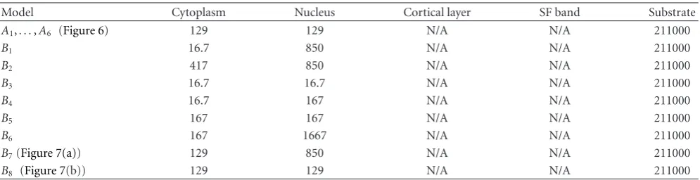
Table1: Material constantC(Pa) in (1) determined for various finite element models.
Model Cytoplasm Nucleus Cortical layer SF band Substrate
A1,. . .,A6 (Figure 6) 129 129 N/A N/A 211000
B1 16.7 850 N/A N/A 211000
B2 417 850 N/A N/A 211000
B3 16.7 16.7 N/A N/A 211000
B4 16.7 167 N/A N/A 211000
B5 167 167 N/A N/A 211000
B6 167 1667 N/A N/A 211000
B7(Figure 7(a)) 129 850 N/A N/A 211000
B8 (Figure 7(b)) 129 129 N/A N/A 211000
ModelsBi(i=1,. . ., 8) have the same profile as modelA1(see left inFigure 5(b)) and a region of the nucleus (seeFigure 7).
material constantCwas defined as 129 Pa for a cell [1] and 211 kPa for the substrate (modelA1inTable 1).
Displacements of±4.53μm (15.1% of the tensile strain) and±0.90μm (3.0% of the compressive strain) were applied to the sides of the substrate as boundary conditions. We obtained these strain values experimentally after all the image acquisitions were complete by averaging the relative
displacements of four ink marks in a 1 × 1 mm square
while the silicone substrate was stretched. These marks were plotted at nine locations in a 10×10 mm square at the center
of the 32×32 mm square membrane. The upper surface of
the substrate (the cell bottom) was held at the same height to obtain the cellular deformation with respect to the substrate surface.
2.7. Error Estimation for Cell Outlines at Various Heights. The average error in the cellular outlines was estimated between the first and second pretest scans and between the experimental data and theoretical predictions. The error was calculated by adding all the areas surrounded by segments of the outline,S1+S2+· · ·+Snand dividing the sum by
the perimeter of the shorter outline for the pretest scans or the perimeter of the theoretical model for the comparison between experimental and theoretical results (seeFigure 2). Rigid body motion was removed by matching the cell bottom outline in an image of the stretched state to that obtained by applying the substrate deformation to the cell bottom outline for the unstretched state. For the finite element analysis results, the two-dimensional (2D) displacement was calculated for nodes at each height range in the unstretched state, that is,h=0 andn−0.05μm≤h≤n+ 0.05μm,n= 1, 2,. . ., neglecting the component in the height direction.
2.8. Sensitivity of the Cellular Deformation to the Elastic-ity of Intracellular Components: A Numerical Study. We investigated the effects of the elasticity of the intracellular components numerically, focusing mainly on the cytoplasm and nucleus during the cell deformation. We prepared finite element models (B1,. . .,B8) with the same geometry as
modelA1and various material constant values
correspond-ing to Young’s moduli for the spread of endothelial cells reported by Caille et al. [1], to investigate the sensitivity of the cellular deformation to the elasticity of the cytoplasm
S1
S2
S3
S4
S5 S6
S7
S8
Figure2: Estimate of the average distance between the two outlines of a cell at each height level: (S1+S2+· · ·+Sn)/perimeter.
and nucleus (seeTable 1). The cytoplasm and nucleus were completely connected at their boundaries. We compared the deformation of the cellular free surface obtained using the above analyses.
The sensitivity to the amount of substrate stretching was also investigated for model A1. With xandy denoted
as the axes of stretching and the transverse directions, respectively, the substrate strains were varied as (εx,εy) =
(0.151,−0.031), (0.101,−0.031), and (0.151, 0).
3. Results
The ratio (r) of the mean intensity in the central 20× 20-pixel region in the second scan to that in the first scan was 0.73±0.05 (mean±SD) for the bottom images of four cells. Table 2summarizes the error estimates for the cell outlines that were identified by theT1andT2threshold values. The
r-value was used to compensate for fluorescence fading in the latter. In the bottom and middle regions, the average error was 0.24 to 0.26μm, or less than one-hundredth of the cell size. The top region had a large average error of 0.44μm, which was significantly different from the average values for the other regions (P < .05 using a statisticalt-test).
(a)
(b)
Figure 3: Fluorescence intensity images of an endothelial cell at heights of 5, 4, 3 (a, left to right), 2, 1, and 0μm (b, left to right), where 0μm is the cell bottom. The cell was stained with calcein-AM. Bar: 20μm.
Table2: Distance error for the outlines of each cell between the first and second measurements using CLSM (n=4). The outline derived from the second measurement was compensated for fluorescent fading.
Region Average (μm) SD (μm) Average±1.28 SD (μm)
Top 0.44 0.14 0.26/0.62
Middle 0.26 0.12 0.11/0.41
Bottom 0.24 0.09 0.13/0.35
The average±1.28 SD covers 90% of the error distribution.
images are located at heights of 5, 4, 3, 2, 1, and 0μm, where 0μm corresponds to the cell bottom. The intensity in the cell region tended to decrease at higher levels.
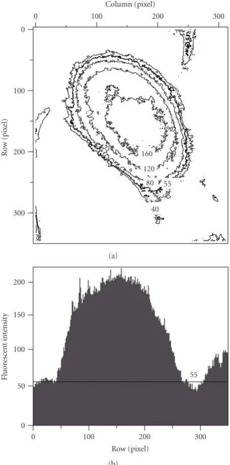
Figure 4(a)shows an example of the fluorescence inten-sity contours at the cell bottom (right image inFigure 3(b)), andFigure 4(b) shows a side view of a surface plot of the intensity. Based on the results in Figure 4(b), the intensity threshold for identifying the cell outline was determined to be 55.
Figure 5shows the geometries of typical finite element models of measured single cells on the substrate before and after stretching. In the geometrical modeling, a small circle was added to the top of the cell at a height of 0.5 or 1.0μm above the highest outline. For the substrate, the edges to the right and left of the figure were stretched by 15.1%, whereas those on the other sides were compressed by 3.0%. The distribution of the maximum principal strain during stretching was plotted on the surfaces of the cell and substrate (right panels inFigure 5).
Table 3 shows the mean and SD of the nominal strain components in the stretching, transverse, and height direc-tions at various height levels of the cell models inFigure 5. The strain components in the stretching and transverse
300 200 100 0
R
o
w
(pix
el)
0 100 200 300
Column (pixel)
160 120
80
40 55
(a)
0 50 100 150 200
Fluor
esc
ent
int
ensit
y
0 100 200 300
Row (pixel)
55
(b)
Figure 4: (a) Contours of the fluorescence intensity at the cell bottom (right image inFigure 3(b)). The thick contour corresponds to the threshold value 55. (b) A side view of the surface plot of the intensity was used to determine the threshold value of 55.
directions were almost equal to the strain of the substrate at the cell bottom; the former strain component decreased gradually, whereas the latter remained relatively constant with increasing height. The strain component in the height direction was 11% compressive in the bottom region and decreased toward zero with increasing height.
0.33 0.3
0.24
0.18
0.12
0.06
0
(a)
0.33 0.3
0.24
0.18
0.12
0.06
0
(b)
Figure5: Geometry of typical finite element models of a cell on the substrate before and after stretching. In the left panels, the substrate is 60-μm-square before stretching. In the right panels, the distribution of the maximum principal strain is also shown for cells when the substrate is stretched in the horizontal direction by 15.1%. The cell in the top line is modelA2, and its profile is made from the images in Figure 3. The cell in the bottom line is modelA1.
Table3: Mean (SD) of nominal strain components in the stretching, transverse, and height directions at various height levels of cell models. The values in the upper and lower rows in the table were obtained from the upper cell model (height: 7μm in the unstretched state) and the lower cell model (height: 5.5μm in the unstretched state) inFigure 5, respectively. The substrate was deformed with strains of 15.1% in the stretching direction and−3% in the transverse direction. Extrapolated values for element nodes from integration-point values were averaged over each height range.
Height ranges (μm) Stretching direction (%) Transverse direction (%) Height direction (%)
0 16.0 (1.0) −3.0 (0.2) −10.8 (0.4)
15.8 (1.0) −2.9 (0.3) −10.7 (0.5)
0.95–1.05 13.4 (1.0) −3.5 (0.6) −8.3 (1.2)
14.0 (1.0) −3.9 (0.6) −8.5 (1.0)
1.95–2.05 11.3 (1.6) −3.5 (0.5) −6.6 (1.5)
13.5 (1.6) −3.9 (0.8) −8.2 (0.7)
2.95–3.05 10.3 (1.2) −3.6 (0.4) −5.9 (1.0)
10.7 (0.6) −3.9 (0.5) −5.9 (1.0)
3.95–4.05 9.2 (1.0) −3.6 (0.4) −4.9 (0.9)
9.3 (0.5) −3.7 (0.3) −4.8 (0.6)
4.95–5.05 7.4 (1.1) −3.4 (0.4) −3.6 (0.9)
8.4 (0.8) −3.7 (0.2) −4.2 (0.6)
5.95–6.05 5.6 (1.4) −3.0 (0.3) −2.2 (1.1)
N/A N/A N/A
figure, the horizontal direction is the stretching direction, and the height interval of each contour is 1μm. The cell was elongated in the substrate-stretching direction, with an associated slight compression in the transverse direction.
Table 4summarizes the distance error between the out-lines obtained from the measurements in the stretched state and those obtained from finite element analyses for six cells. In the third column, the relative error of the displacement is listed with respect to the mean 2D displacement of the cellular free surface at the same height level. For the lower
half of the cells, the average distance error was 0.41 to 0.55μm, or 24% to 48% of the mean displacement at the same height level, whereas these values were 0.86 to 1.28μm or 128% to 278% for the upper half of the cells. Such large relative errors resulted from dividing the distance error by a small mean displacement which decreased toward zero with increasing height.
A1 A2
A3 A4
A5 A6
Unstretched state
(a)
A1 A2
A3 A4
A5 A6
Stretched state
(b)
Figure6: Comparisons of (a) contours measured in the unstretched state (blue lines) and those smoothed to make the 3D geometric models (red lines), and (b) contours measured in the stretched state (blue lines) and those predicted by the finite element analysis (red lines). The height interval between adjacent outlines is 1μm. Bar: 20μm.
Table4: Distance error for the outline of each cell in the stretched state between the CLSM measurement and the results of the finite element analysis (n=6). At each height level for cells in the finite element analysis, the 2D mean displacement was calculated excluding the displacement component in the height direction.
Region Average (SD) (μm) Average (SD) with respect
to mean displacement (%)
Top 1.28 (0.78) 278 (100)
Middle (upper half) 0.86 (0.43) 128 (65)
Middle (lower half) 0.55 (0.19) 48 (24)
Bottom 0.41 (0.12) 24 (7)
elasticity, which was (a)C = 850 Pa and (b) C = 129 Pa.
In Figure 7(a), the deformed model B7 had two
peak-displacement regions in the free-surface regions due to the stiff nucleus. In Figure 7(b), the deformed model B8
had almost horizontal isodisplacement lines, showing near uniform deformation at each height level.Figure 7(c) com-pares the displacement in the stretching direction in the major cross-section between modelsB7 (top panel) andB8
(bottom panel). The stiffnucleus restricted the deformations of itself and the cytoplasm in its vicinity, decreasing the height reduction of the cellular top and the nuclear elon-gation in the stretching direction when the substrate was stretched.
The sensitivity of the deformation of the cellular free sur-face to the elasticity of the cytoplasm and nucleus was eval-uated. The difference between the 2D displacement of nodes
(height≥0 in the unloaded state) on the cellular free surface
in modelsB1 andB2 was 0.069±0.077μm or 5.6±6.2%
(mean ±SD) compared to the mean 2D displacement of
these nodes. Among modelsB1,. . .,B8, the maximum diff
er-ence was 0.090±0.098μm or 7.2±7.9% (B1versusB3,B5, or
B8; modelsB3,B5, andB8had identical displacements). These
errors were smaller than the spatial resolution of the images. The sensitivity of the deformation of the cellular free surface to the magnitude of substrate stretching was also
evaluated using model A1. The difference between the
substrate stretching and the mean 2D displacement of the nodes on the cellular free surface (height>0 in the unloaded state) was 0.49±0.31μm and 33±21% (mean±SD) between
εx = 0.151 and 0.101 with a constant εy = −0.031, and
0.3±0.15μm and 15±10% betweenεy= −0.031 and 0 with
(μm) 0.025
−0.075
−0.175
−0.275
−0.375
−0.475 (a)
(μm) 0.025
−0.075
−0.175
−0.275
−0.375
−0.475 (b)
(μm) 5 4 3 2 1 0
−1
−2
−3
−4
−5 (c)
Figure7: Comparisons of (a) the displacement in the height direction along the major and minor cross-sections for modelB7and (b) model
B8; (c, top panel) displacement in the stretching direction along the major cross-section for modelB7and (c, bottom panel) modelB8under 15.1% stretching of the substrate associated with 3.0% transverse compression. In the figure, the substrate is stretched symmetrically in the right and left directions.
4. Discussion
Published studies on the deformation of an entire cell typ-ically analyzed cellular deformation independent of height position [2–6]. In confocal sectioning of chondrocytes, the outlines were compared between the uncompressed and compressed states only in the central plane of each cell [7]. Furthermore, in image-based 3D modeling of cells [8, 10, 16], the geometric change of an entire cell with the application of force or displacement that was seen in a numerical analysis was not compared with experimental results. By contrast, we obtained a contour map of cells in the unstretched and stretched states, enabling an analysis of the height-dependent deformation. Then, we compared the outline of cells on the substrate surface between the unstretched and stretched states, considering the deforma-tion of the substrate. We also made finite element models and compared the theoretically predicted profiles with experimentally obtained outlines of cells at different heights.
These techniques will lead to more accurate understanding of the three-dimensional deformation of cells subjected to various forces and displacements.
Experimental and theoretical analyses of cellular defor-mation indicate that a hyperelastic material model is a practical approximation for describing the deformation of a cell after quasistatic stretching after completion of the stress relaxation. A finite element model by Yamada et al. [17] consisting of a neo-Hookean plasma membrane and incompressible cytoplasm caused slight buckling of the cel-lular free surface under uniaxial stretching of the substrate. Solid constituents in the cytoplasm must be requisite to support the flexible plasma membrane. Our model expressed the cytoplasm as a neo-Hookean material, which is more appropriate for describing the cell deformation.
boundary of a fluorescent bead. Thus, it is necessary to determine a threshold value for the cell boundary. We confirmed that well-determined thresholds in images before and after stretching indicate the same boundary. Although a threshold might define a larger or smaller region than the actual cell boundary, the cell body defined using the threshold is made of the same material.
There are fluorescent dyes that label the plasma mem-brane to identify a cell border. To the best of our knowledge, however, these have not been used for the purpose of extracting the 3D border from adherent cells. Such dyes might not be suitable for staining the fine details of all parts of the plasma membrane of adherent cells, both at the free surface and the cell bottom.
According to Table 4, our cell body model could be
used to provide a practical reproduction of the cellular deformation, with possible small errors in the boundary for the lower half of the cell but significant errors for the upper half. This might have been due to a lack of volume with sufficient fluorescence intensity in the top region of a cell. By comparing the right image inFigure 3(b)and the contour labeled “55” inFigure 4(a), it is evident that lamellipodia and filopodia were not included in the 3D geometrical model. The volume of these podia was too small for the fluorescence intensity to be detected above the threshold.
A 20×20-pixel region in the cell bottom image was
theoretically deformed to a 23×19.4-pixel region by the substrate deformation. Between these pixel regions, 70 pixels sharing 18% of the region were not identical. We ignored the error resulting from this difference because the 20×20-pixel region at the central portion of the cell bottom had a small fluorescence intensity gradient (seeFigure 4). A complicated procedure would be required to determine the fluorescence fading rate between the unstretched and stretched states.
The basic models in the present study (modelsA1,. . .,
A6) assumed a homogeneous material due to the lack of
data on microscopic or regional material properties. A cell consists of various organelles, such as the nucleus and cytoskeleton. Of these organelles, the nucleus has the greatest effect on the cell deformation. The displacement of the free surface differed by<0.1μm or 7% of the mean displacement of nodes from that of the nucleus-free model under substrate stretching. This difference is at most one-fifth of the error in the lower region of cells in the experiment (seeTable 4).
In reality, an endothelial cell consists of viscoelastic material [19], and its mechanical properties change when it remodels [20]. No well-defined 3D viscoelastic material model has yet been established, and the remodeling process has not been incorporated into a constitutive or structural model, which remains as a future problem.
In the present study, we only applied displacement boundary conditions and assumed a simple nucleus geom-etry, referring to the finite element model in Caille et al. [1]. Force boundary conditions, such as cell poking, should be considered to validate the material properties in the finite element model. The geometry and location of the nucleus are also important factors to describe the mechanical states of intracellular components. Modeling of cells on the basis of
double- or multistaining image data for the cytoplasm and nucleus, and considering stress fibers and focal adhesions, remain as areas of future study.
Prestress in the cytoskeletal network has been incor-porated in the tensegrity model, which is a representative unit of the cytoplasm [16, 21]. So far, our finite element models represent homogenized behavior in the cytoplasm. Reproducing the microscopic stress distribution in cytoskele-tal components is an area of future study that will also incorporate pretension in actin filaments.
5. Conclusion
This is the first study to measure and validate the 3D geomet-rical change of adherent cells when the substrate is stretched. The advantages of the 3D measurement and numerical deformation analysis are that they provide detailed data on the cellular deformation according to the height position, reflecting the cellular shape. We also analyzed the sensitivity of the elasticity of intracellular components on the cellular deformation. The present study provides a basis of adequate finite element modeling of cells under stretching of the vascular wall or substrate to investigate effects caused by the mechanical environment. Future studies should measure and model the cellular structure precisely and also reproduce the mechanical fields to correlate with intracellular responses such as stress fiber formation.
Acknowledgment
This study was partially supported by a Grant-in-Aid for Scientific Research on Priority Areas (no. 15086213) from the Ministry of Education, Culture, Sports, Science, and Technology of Japan.
References
[1] N. Caille, O. Thoumine, Y. Tardy, and J.-J. Meister, “Contribu-tion of the nucleus to the mechanical properties of endothelial cells,” Journal of Biomechanics, vol. 35, no. 2, pp. 177–187, 2002.
[2] K. A. Barbee, E. J. Macarak, and L. E. Thibault, “Strain measurements in cultured vascular smooth muscle cells subjected to mechanical deformation,”Annals of Biomedical Engineering, vol. 22, no. 1, pp. 14–22, 1994.
[3] N. Caille, Y. Tardy, and J.-J. Meister, “Assessment of strain field in endothelial cells subjected to uniaxial deformation of their substrate,”Annals of Biomedical Engineering, vol. 26, no. 3, pp. 409–416, 1998.
[4] S. I. Simon and G. W. Schmid-Sch¨onbein, “Cytoplasmic strains and strain rates in motile polymorphonuclear leuko-cytes,”Biophysical Journal, vol. 58, no. 2, pp. 319–332, 1990. [5] C. L. Gilchrist, S. W. Witvoet-Braam, F. Guilak, and L. A.
Setton, “Measurement of intracellular strain on deformable substrates with texture correlation,”Journal of Biomechanics, vol. 40, no. 4, pp. 786–794, 2007.
[7] D. A. Lee, M. M. Knight, J. F. Bolton, B. D. Idowu, M. V. Kayser, and D. L. Bader, “Chondrocyte deformation within compressed agarose constructs at the cellular and sub-cellular levels,”Journal of Biomechanics, vol. 33, no. 1, pp. 81–95, 2000. [8] T. Ohashi, H. Sugawara, T. Matsumoto, and M. Sato, “Surface topography measurement and intracellular stress analysis of cultured endothelial cells exposed to fluid shear stress,”JSME International Journal, Series C, vol. 43, no. 4, pp. 780–786, 2000.
[9] G. T. Charras and M. A. Horton, “Determination of cellular strains by combined atomic force microscopy and finite element modeling,”Biophysical Journal, vol. 83, no. 2, pp. 858– 879, 2002.
[10] M. C. Ferko, A. Bhatnagar, M. B. Garcia, and P. J. Butler, “Finite-element analysis of a multicomponent model of sheared and focally adhered endothelial cells,” Annals of Biomedical Engineering, vol. 35, pp. 208–223, 2007.
[11] H. Yamada, D. Morita, J. Matsumura, T. Takemasa, and T. Yamaguchi, “Numerical simulation of stress fiber orientation in cultured endothelial cells under biaxial cyclic deformation using the strain limit hypothesis,”JSME International Journal, Series C, vol. 45, no. 4, pp. 880–888, 2002.
[12] H. Yamada and J. Matsumura, “Finite element analysis of the mechanical behavior of a vascular endothelial cell in culture under substrate stretch,”Transactions of JSME, Series A, vol. 70, no. 5, pp. 710–716, 2004 (Japanese).
[13] R. P. Jean, C. S. Chen, and A. A. Spector, “Finite-element anal-ysis of the adhesion-cytoskeleton-nucleus mechanotransduc-tion pathway during endothelial cell rounding: axisymmetric model,”Journal of Biomechanical Engineering, vol. 127, no. 4, pp. 594–600, 2005.
[14] P. Tracqui and J. Ohayon, “Transmission of mechanical stresses within the cytoskeleton of adherent cells: a theoretical analysis based on a multi-component cell model,” Acta Biotheoretica, vol. 52, no. 4, pp. 323–341, 2004.
[15] H. Yamada and H. Ando, “Orientation of apical and basal actin stress fibers in isolated and subconfluent endothelial cells as an early response to cyclic stretching,”Molecular and Cellular Biomechanics, vol. 4, no. 1, pp. 1–12, 2007.
[16] D. Stamenovic, “Effects of cytoskeletal prestress on cell rheological behavior,”Acta Biomaterialia, vol. 1, no. 3, pp. 255–262, 2005.
[17] H. Yamada, H. Ishiguro, and M. Tamagawa, “Mechanical behavior and structural changes of cells subjected to mechan-ical stimuli: deformation, freezing, and shock waves,” in Biomechanics at Micro- and Nanoscale Levels, H. Wada, Ed., vol. 1, pp. 154–164, World Scientific, Singapore, 2005. [18] E. A. G. Peeters, C. V. C. Bouten, C. W. J. Oomens, D. L.
Bader, L. H. E. H. Snoeckx, and F. P. T. Baaijens, “Anisotropic, three-dimensional deformation of single attached cells under compression,”Annals of Biomedical Engineering, vol. 32, no. 10, pp. 1443–1452, 2004.
[19] M. Sato, N. Ohshima, and R. M. Nerem, “Viscoelastic properties of cultured porcine aortic endothelial cells exposed to shear stress,”Journal of Biomechanics, vol. 29, no. 4, pp. 461– 467, 1996.
[20] R. M. Nerem and D. Seliktar, “Vascular tissue engineering,” Annual Review of Biomedical Engineering, vol. 3, pp. 225–243, 2001.