A search space optimization technique for improving ambiguity resolution and
computational efficiency
Donghyun Kim and Richard B. Langley
Geodetic Research Laboratory, Department of Geodesy and Geomatics Engineering, University of New Brunswick, Fredericton, N.B., Canada
(Received January 5, 2000; Revised June 24, 2000; Accepted July 9, 2000)
An Optimal Method for Estimating GPS Ambiguities (OMEGA) that enables very high performance and com-putational efficiency has been developed and demonstrated. This method employs two search space reduction processes—a scaling and a screening process—that are related to the search space transformation and the ambi-guity candidate filtering in multi-search levels. To obtain the highest efficiency, an optimization procedure, which determines the parameters to minimize the number of candidates under given conditions, is implemented in closed-form before the search-verification step. The method is essentially based on the least-squares-approach originally proposed by Hatch but uses a modified and more efficient process. Two improved algorithms are introduced in this paper. First, an alternative algorithm for the spectral decomposition, which reduces the dimension of the residuals vector to its degrees of freedom, is given in closed form. This algorithm is implemented in the computational step of the quadratic form of the residuals in order to increase computational efficiency. Second, an efficient error model for the threshold of the filter equation that is used to derive the search space scaling process is given. This error model shows two advantages: 1) it bounds noise signals of the filter equation; 2) it gives efficient thresholds so that the scaling effects for the search space can be increased.
1.
Introduction
In navigation and surveying systems using GPS carrier phase data, the performance of ambiguity resolution and computational efficiency are of great concern. These capa-bilities are often traded off in designing the system. One possible way to overcome the trade-off loss is to reduce the number of ambiguity candidates before or at the search-verification step. The search space transformation (Abidin, 1993; Teunissen, 1994; Martin-Neiraet al., 1995) and am-biguity candidate filtering in multi-search levels (Chen and Lachapelle, 1995; Teunissen, 1997) are effective techniques for that purpose.
When we use a process similar to the least-squares-ap-proach of Hatch (1990) at the search-verification step, it is possible to implement optimization procedures reducing the number of candidates before implementing the step. We showed that this could be achieved using the design matrix of the linearized double-difference observables in Kim and Langley (1999). These optimization procedures include two search-space reduction processes (i.e., a scaling and a screen-ing process) and two-step optimization processes—a global optimization to find a matrix S minimizing the total search space volume and a local optimization to find a reordered matrix S minimizing the total search space volume out of all possible combinations of S, where the matrix S is computed using the design matrix.
To increase computational efficiency, further attention has been given to the quadratic form of the residuals and to error
Copy right cThe Society of Geomagnetism and Earth, Planetary and Space Sciences (SGEPSS); The Seismological Society of Japan; The Volcanological Society of Japan; The Geodetic Society of Japan; The Japanese Society for Planetary Sciences.
models for the thresholds of the filter equation. The quadratic form of the residuals is generally used for the ambiguity ac-ceptance test and is the practical computational part in the ambiguity search-verification step. Therefore, we need to decrease computational burden using a more efficient com-putational algorithm. A significant reason for needing a more efficient error model for the filter thresholds is that the filter thresholds are related to a magnification factor of the scaling process. The more efficient the error model, the greater the scaling effect.
1.1 The GPS observables
To simplify discussions, we will assume that the float esti-mates of the ambiguities and their error models are given. For the double-difference observables recorded on short base-lines, the satellite and the receiver clock biases are removed, and the residual atmospheric effects are negligible. Ignoring multipath, we have
l=Ax+N+e
E[e]=0, Cov[e]=Q, (1)
wherelis then×1 initial misclosure vector of the difference between the double-difference observations and their esti-mates;nis the number of the double-difference observations;
xis the 3×1 vector of the unknown remote (rover) station position components;Ais the design matrix for the unknown position;Nis then×1 vector of ambiguity parameters;eis then×1 vector of the double-difference observation noise;
E[·] and Cov[·] represent the mathematical expectation and the variance-covariance operators, respectively.
Table 1. Modified least-squares-approach.
Processing Computational equations
steps Original approach Modified approach
Potential solutions xp=A−1
p (lp−Np) xp= −A− 1 p Np Np∈⺪3
Secondary ambituities S=AsA−1 p
1.2 The modified least-squares approach
Using the same terminology as Hatch (1990), we outline the modified process for the least-squares approach in Ta-ble 1. In the computational equations, the subscripts“p”
and“s”represent the primary and the secondary group of satellites; and round[·] is the rounding-to-the-nearest-integer operator.
When compared with the original least-squares approach, the modified approach gives exactly the same residuals. To prove the equivalence of both approaches, we will define:
δxp=A−p1lp
ls=Asδxp=Slp.
(2)
Then, we have following equality:
A∗
Subtracting the residuals for both approaches and applying Eq. (3) gives
v=vm−vo
=(I−AA∗)(lm −lo)=0, (4)
where subscripts“o”and“m”represent the original and mod-ified approaches.
1.3 Thefilter equation for the secondary innovations vector
When we compute the residuals using the modified ap-proach in Table 1, the only variable parameter is the sec-ondary innovations vector. In accord with the least-squares principle, the optimal estimator for the secondary innovations vector is given as:
∂(vTQ−1v)
∂ls =0, ∴ˆl
s=Slp. (5)
We can recognize that the optimal estimator is independent of the search-verification step, since it is derived from the design matrix and the initial misclosure vector for the primary group. These parameters are constant in a snapshot (i.e., single epoch) approach, such as the least-squares approach.
One natural idea to utilize the optimal estimator is to define afilter equation as:
w=ls− ˆls
=ls−S(lp−Np)−round[ls−S(lp−Np)]. (6)
Using thefilter equation and a certain threshold vectorτ, we can define afilter as:
The dimension ofn−3 for thefilter equation and thresh-old vector comes from the dimension difference between the (n-dimensional) double-difference observations and the (3-dimensional) unknown remote station position components.
2.
Quadratic Form of the Residuals
For the ambiguity acceptance test, we have to compute the quadratic form of the residuals for all ambiguity candidates in the ambiguity search-verification step. Two approaches can be considered for decreasing computational burden—search space (or ambiguity candidates) reduction and computational algorithm improvement. We will focus on the computational algorithm for the quadratic form of the residuals in this paper. Using the computational equation for the residuals in Table 1, the quadratic form of the residuals is given as:
vTQ−1v=lTl, (9)
where
=(I−AA∗)TQ−1(I−AA∗). (10) Spectral decomposition for a singular symmetric matrix
is expressed as (Basilevsky, 1983):
=EET, (11)
where then ×(n −3)matrixEcontains then ×1 latent vectors (eigenvectors)E1,E2, . . . ,En−3 and the(n−3)×
Table 2. Comparison of the computational algorithms. We canfind an example of this algorithm in Martin-Neira et al.(1995). An alternative algorithm for the spectral de-composition approach can be derived using the following relational equations. From Eq. (4), rewriting the residuals gives
Therefore, using the partitioned matrices ofG=I−AA∗, we have two relational equations from Eq. (14) as:
vp =GpsG−ss1vs (15)
vs =Gssw. (16)
Using the partitioned matrices ofP=Q−1, the quadratic form of the residuals can be expressed as:
vTQ−1v=vTpPppvp+vTsPspvs+vTsPssvs. (17)
Furthermore, the following equality can be proved:
R=Q−V1
ss, (20)
whereQVssis a partitioned matrix of the variance-covariance ofv,Qv.
To compare the computational efficiency of different algo-rithms, we outline three algorithms for the computation of the quadratic form of the residuals in Table 2. The computational algorithms A1 and A2 represent a normal and a spectral de-composition approach. The computational algorithm A3 is an alternative approach for the computational algorithm A2.
The computational steps are separated into three parts for clarity—common, external, and internal. The external part is computed before the ambiguity search-verification step. On the other hand, the internal part is computed in the search loop. Therefore, the computational efficiency of the internal part is usually of great concern.
3.
Error Model for the Filter Threshold
In general, the threshold vectorτ in Eq. (7) can be derived from the quadratic form of thefilter equation as:
wTQ−w1w≤c, (21)
whereQwis the variance-covariance matrix ofwandcis a
positive constant which can be selected based on the prob-ability distribution ofw. Therefore, we can determine
con-fidence intervals bounding a confidence ellipsoid which is formed by choosingcat a certain confidence level. Then, one simple way to set the thresholds is
τi =σwi
√
c, i =1,2, . . . ,n−3 (22)
where σwi is the square root of the ith diagonal element inQw. It should be noted that the confidence level of the
thresholds is different from that of the confidence ellipsoid. (When we mention a confidence level in this paper, it refers to the confidence ellipsoid.) However, we can recognize in Eq. (6) that it is not easy to establish correctly the variance-covariance matrixQwand the probability distribution ofw.
For this reason, we have used an alternative approach for the quadratic form of the filter equation. In general, the ellipsoidal region in⺢n−3 centered on the estimatorxˆ of a certain vectorxcan be expressed as (Giri, 1977):
(x− ˆx)TQx−ˆ1(x− ˆx)≤c, (23)
whereQxˆ is the variance-covariance matrix ofxˆ. The family of ellipsoids obtained by varying c(c > 0)has the same centerxˆ, their shapes and orientation are determined byQxˆ, and their sizes are determined byc. It should be noted that the positive constantcdoes not have probabilistic sense unless the probability distribution ofxis known. From Eq. (23), the thresholds are given as:
τi =σxiˆ
√
c, i =1,2, . . . ,n−3 (24)
Table 3. Error models for thefilter thresholds.
x xˆ orw Qxˆ orQw
(a) round[y]+S(lp−Np) ls Qss
(b) round[y] y Qss+SQppS
T
−SQps−QspST
(c) ls ˆls SQppST
(d) — G−1
ssvs G−ss1QVssG− T ss
Fig. 1. Canadian Coast Guard DGPS and OTF network: coverage of the St. Lawrence River. Test data were recorded at the Trois-Rivi`eres reference station and a hydrographic sounding ship on September 30, 1998.
ˆ
x should be the unbiased estimator ofx; then, we can get different thresholds according to the weighting scheme of
Qxˆ. Three cases from (a) to (c) in Table 3 show the unbiased estimators ofxand their error models. Because bothxand
ˆ
xare probabilistic variables, the condition of unbiasedness becomes
E[x]=E[xˆ]. (25)
For each case, the condition of unbiasedness can be proved if the following equality holds (more details in Teunissen (1998)):
E[round[y]]=SNp, (26)
where
y=ls−S(lp−Np). (27)
Three error models for thefilter thresholds (i.e., the error models from (a) to (c)) were tested and discussed in Kim and Langley (1999). A rigorous error model, which is related to deciding the value of the positive constantcin a probabilistic sense, can be derived from Eqs. (18) and (21). From these two equations, we can express a correct error model of the
filter equationwas:
Qw=−1=G−ss1QVssG −T
ss . (28)
Assuming that the double-difference observation noisee
in Eq. (1) has a normal distribution, we have
vTQ−1v=wTQw−1w∼χ2(n−3, α), (29)
whereαis the level of significance. Therefore, we can deter-mine the positive constantcwith a certain confidence level in accord with α. Table 3 shows the summary of the er-ror models for the filter thresholds. In each error model, the variance-covariance matrices with subscripts are the sub-matrices partitioned from the variance-covariance matrix of the double-difference observations in Eq. (1).
4.
Results
To test the efficiency of the computational algorithms for the quadratic form of the residuals and the performance of the error models for thefilter thresholds, we processed some of the test data recorded at one reference station in the Cana-dian Coast Guard (CCG) DGPS and OTF network and that recorded simultaneously on board a hydrographic sounding ship at Trois-Rivi`eres, on the St. Lawrence River, 130 km up-stream (southwest) of Quebec City, on September 30, 1998´
(Fig. 1). The data set contains both L1 and L2 observations recorded at a one second sampling interval for two hours in kinematic mode. Baseline length between the reference station and hydrographic sounding ship was about 40 km.
Table 4. FLOPS test results.
A1 A2 A3
Common 1,588
External 868 5,278 1,040
Internal 1,917,027 722,358 694,575
Total 1,919,483 729,674 697,203
floating point operation count (FLOPS) test of the computa-tional algorithms for the quadratic form of the residuals; and the performance of the error models for thefilter thresholds.
4.1 Computational algorithm efficiency
Using each computational algorithm for the quadratic form of the residuals in Table 2, the FLOPS test was conducted to compare the efficiency of the algorithms. (Although this test cannot give us a realistic computation time, we can see the relative efficiencies of the algorithms.) Table 4 shows the test results. Test conditions were given as: 1) three-level search loops were built; 2) the search range for each search level was given as 2 m, therefore, twenty-one candidates were given for each search level; 3) seven satellites were used.
The normal computational algorithm A1 gave the worst computational efficiency and the alternative algorithm A3 for the spectral decomposition approach gave the best results. Compared with the normal algorithm A1, the efficiency of the spectral decomposition algorithm A2 was improved by about 62%. In the case of the alternative algorithm A3, the efficiency was improved by about 64%. In both the exter-nal and interexter-nal computation parts, the alternative algorithm A3 was superior to the spectral decomposition algorithm A2. We have obtained consistent results under different test con-ditions. We can say therefore, that the alternative algorithm A3 is the most efficient algorithm of the three algorithms tested for computing the quadratic form of the residuals no matter which test conditions are given.
4.2 Error model performance
To compare the performance of the error models, thefilter thresholds were computed using Eqs. (22) and (24) for each error model in Table 3. The positive constant valuecwas determined from the chi-squared distribution at the 95%
con-fidence level withn−3 degrees of freedom (i.e., we assumed that the double-difference observation noise follows the nor-mal distribution). As was mentioned previously, however, this choice ofccannot guarantee the same confidence level to the error models from (a) to (c) in Table 3, because these er-ror models are not based on a rigorously-defined probability distribution. Even though this limitation exists, we consid-ered, as a matter of convenience, that the positive constant chas the same confidence level for all error models in our investigations.
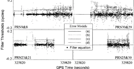
Figure 2 shows the overall performance of the error mod-els, i.e., how well thefilter thresholds (solid lines) bound the values of thefilter equation (dots). To investigate the per-formance of the error models in detail, we plotted thefilter thresholds for each error model and for the double-difference time series of PRN 9 and 8 separately in Fig. 3. We need in
Fig. 2. Overall performance analysis of the error models (95% confidence level): Only positive threshold values are plotted for simplicity. The
filter thresholds bound the values of thefilter equation for each dou-ble-difference time series in order to guarantee a reduced search space including true ambiguities within the given confidence level.
Fig. 3. Performance comparison of the error models for the PRN 9&8 double-difference time series (95% confidence level): The error models from (a) to (d) are defined in Table 3.
general an error model that protects all the values of thefilter equation for true ambiguities in the given confidence level, which at the same time is also efficient. The third error model satisfies these criteria as shown by the examples in Fig. 3. On the other hand, it is evident that thefirst error model does not satisfy these criteria. Furthermore, thefirst error model did not react well to the noise level of thefilter equation. For the second and fourth error models, our investigations have shown that both of these error models have similar character-istics (sometimes, almost identical). In fact, the equation for the fourth error model can be developed in a similar form to that of the second error model in Table 3. According to the partitioned design matrices, both error models would be al-most identical. The performance of these error models is not much different from that of the third error model as shown by the examples in Fig. 3.
5.
Conclusions
for the spectral decomposition is the most efficient. Regard-ing the error models for thefilter thresholds in Table 3, we found that three of the four error models performed well, i.e., thefilter thresholds bounded almost all the noise signals of thefilter equation. Only thefirst of the four performed poorly. We also found that the second and fourth error mod-els have similar behavior. However, because of the meaning of the positive constantc(i.e., for robustness, it should be determined not arbitrarily but in a probabilistic sense), we have considered the fourth error model as the most rigorous approach in our investigations.
Acknowledgments. This work has been conducted under the GEOIDE Network of Centres of Excellence (project ENV#14). The support of the Canadian Coast Guard; the Canadian Hydrographic Service; VIASAT G´eo-Technologie Inc.; Geomatics Canada; and the Centre de Recherche en G´eomatique, Universit´e Laval is grate-fully acknowledged. Thefirst author also thanks the Korea Re-search Foundation for support under its post-doctoral fellowship program while staying in the University of Maine, U.S.A. We are also grateful for useful comments on this paper received from Prof. B. Hofmann-Wellenhof, Dr. Peiliang Xu and an anonymous reviewer.
References
Abidin, H. Z., On the construction of the ambiguity searching space for
on-the-fly ambiguity resolution,Navigation: Journal of The Institute of Navigation,40(3), 321–338, 1993.
Basilevsky, A.,Applied Matrix Algebra in the Statistical Sciences, Elsevier Science Publishing Co., Inc., 389 pp., North-Holland, New York, 1983. Chen, D. and G. Lachapelle, A comparison of the FASF and least-squares
search algorithms for on-the-fly ambiguity resolution,Navigation: Jour-nal of The Institute of Navigation,42(2), 371–390, 1995.
Giri, N. C.,Multivariate Statistical Inference, 319 pp., Academic Press, New York, 1977.
Hatch, R., Instantaneous ambiguity resolution, Proceedings of KIS’90, Banff, Canada, September 10–13, pp. 299–308, 1990.
Kim, D. and R. B. Langley, An optimized least-squares technique for im-proving ambiguity resolution performance and computational efficiency, Proceedings of ION GPS’99, Nashville, Tennessee, September 14–17, pp. 1579–1588, 1999.
Martin-Neira, M., M. Toledo, and A. Pelaez, The null space method for GPS integer ambiguity resolution, Proceedings of DSNS’95, Bergen, Norway, April 24–28, Paper No. 31, 8 pp., 1995.
Teunissen, P. J. G., A new method for fast carrier phase ambiguity estima-tion, Proceedings of IEEE PLANS’94, Las Vegas, Nevada, April 11–15, pp. 562–573, 1994.
Teunissen, P. J. G., A canonical theory for short GPS baselines. Part III: The geometry of the ambiguity search space,J. Geod.,71(8), 486–501, 1997.
Teunissen, P. J. G., A class of unbiased integer GPS ambiguity estimators, Artificial Satellites,33(1), 3–10, 1998.