FULL PAPER
Coseismic deformation due to the 2011
Tohoku-oki earthquake: influence of 3-D elastic
structure around Japan
Akinori Hashima
1*, Thorsten W. Becker
2,3, Andrew M. Freed
4, Hiroshi Sato
1and David A. Okaya
2Abstract:
We investigated the effects of elastic heterogeneity on coseismic deformation associated with the 2011 Tohoku-oki earthquake, Japan, using a 3-D finite element model, incorporating the geometry of regional plate boundaries. Using a forward approach, we computed displacement fields for different elastic models with a given slip distribution. Three main structural models are considered to separate the effects of different kinds of heterogeneity: a homogeneous model, a two-layered model with crust–mantle stratification, and a crust–mantle layered model with a strong sub-ducting slab. We observed two counteracting effects: (1) On large spatial scales, elastic layering with increasing rigid-ity with depth leads to a decrease in surface displacement. (2) An increase in rigidrigid-ity from above the slab interface to below causes an increase in surface displacement, because the weaker hanging wall deforms to accommodate coseismic slip. Results for slip inversions associated with the Tohoku-oki earthquake show that slip patterns are modi-fied when comparing homogeneous and heterogeneous models. However, the maximum slip only changes slightly: It increases from 38.5 m in the homogeneous to 39.6 m in the layered case and decreases to 37.3 m when slabs are introduced. Potency, i.e., the product of slip and fault area, changes accordingly. Layering leads to inferred slip distri-butions that are broader and deeper compared to the homogeneous case, particularly to the south of the overall slip maximum. The introduction of a strong slab leads to a reduction in slip around the slip maximum near the trench. We also find that details of the vertical deformation patterns for heterogeneous models are sensitive to the Poisson’s ratio. While elastic heterogeneity does therefore not have a dramatic effect on bulk quantities such as inferred potency, the mechanical response of a layered medium with a slab does lead to a systematically modified slip response, and such effects may bias studies of mega-thrust earthquakes.
Keywords: 2011 Tohoku-oki earthquake, Elastic structure, Finite element model, Slip inversion, GPS observation
© 2016 The Author(s). This article is distributed under the terms of the Creative Commons Attribution 4.0 International License (http://creativecommons.org/licenses/by/4.0/), which permits unrestricted use, distribution, and reproduction in any medium, provided you give appropriate credit to the original author(s) and the source, provide a link to the Creative Commons license, and indicate if changes were made.
Introduction
The 2011 M9 Tohoku-oki earthquake, Japan, is one of the largest earthquakes ever observed, causing an abrupt change in regional seismicity and large-scale crustal deformation (e.g., Nishimura et al. 2011; Ishibe et al.
2011; Fig. 1). Given the mandate of improving our under-standing of the associated seismic hazard, and utilizing the well-instrumented deformation signatures of this earthquake for our understanding of crustal mechanics,
it is important to understand the coseismic slip, and how it may be influenced by the heterogeneity of the elastic structure that surrounds the plate interface.
The coseismic slip of the Tohoku-oki earthquake has been estimated from various observations including tel-eseismic waveforms (e.g., Yagi and Fukahata 2011), strong motion (e.g., Suzuki et al. 2011), and tsunami propaga-tion (e.g., Fujii et al. 2011), as well as from geodesy. The Japanese islands are covered with one of the world’s most dense GPS networks and seafloor geodetic stations that recorded coseismic surface displacements caused by the earthquake (Fig. 1). A number of geodetic slip inver-sions have been published, most of which used response (Green’s) functions computed with the assumption of a
Open Access
*Correspondence: hashima@eri.u-tokyo.ac.jp
1 Earthquake Research Institute, University of Tokyo, Yayoi 1-1-1,
Bunkyo-ku, Tokyo 113-0032, Japan
Page 2 of 15 Hashima et al. Earth, Planets and Space (2016) 68:159
homogeneous elastic half-space (e.g., Ozawa et al. 2011,
2012; Iinuma et al. 2011, 2012; Perfettini and Avouac
2014), which is often an adequate approximation. How-ever, the great spatial extent of the Tohoku-oki earth-quake, more than 500 km along the surface, causing stress changes to similar depth extent, makes it likely that the resulting surface deformation was affected by the het-erogeneity of the surrounding structure. Those include lateral variations in elastic strength due to the presence of the slab as well as depth dependence due to the influ-ence of pressure and temperature on elastic strength.
For example, the consideration of elastic moduli increas-ing with depth may lead to an increase in inferred seis-mic moment compared to a homogeneous model (e.g., Hearn and Bürgmann 2005; Pollitz et al. 2011; Diao et al.
2012; Dong et al. 2014). Conversely, the consideration of a strong slab (a slab with increased rigidity) in the coseis-mic inversion was shown to lead to a decrease in inferred seismic moment compared to a homogeneous model (Hsu et al. 2011; Kyriakopoulos et al. 2013). Considera-tion of surface topography and lateral heterogeneity from seismic tomography was also found to lead to a better fit to the observed coseismic surface displacements (Pul-virenti et al. 2014; Romano et al. 2014). There is, however, significant uncertainty when seismic velocity is con-verted to elastic moduli because of the possibly compet-ing effects of temperature, pressure, and composition. Moreover, the physical mechanisms as to how different kinds of elastic heterogeneity affect surface deformation are unclear.
Here, we develop a 3-D finite element model that sys-tematically investigates the kinematics of the Tohoku-oki earthquake given different structural configurations in order to understand how the various components influ-ence the inferred slip distribution and seismic moment. This complexity includes depth-dependent elastic struc-ture (including a Moho interface), as well as the incor-poration of both the Pacific (PAC) and Philippine Sea Plate (PHS) slabs. We also study what level of complex-ity may be required to accurately explain both horizon-tal and vertical onland GPS, as well as seafloor geodetic observations.
Methods
We model elastic structure corresponding to crust–man-tle layering under northeast Japan on the Eurasian plate (EUR) and the descending PAC and PHS slabs with a finite element method. Effects of elastic structure on coseismic deformation are evaluated by the following steps: (1) compute deformation due to a slip distribu-tion given by a simple model to resemble the actual slip distribution of the Tohoku-oki earthquake for different structures (forward test) in order to get an understand-ing of the characteristic patterns and (2) invert for the actual slip distributions based on the data using Green’s functions for slip patches computed for different elastic structures.
Finite element modeling
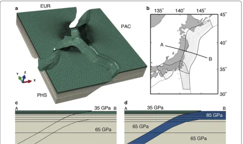
We use the ABAQUS finite element modeling software (http://www.3ds.com) to model coseismic deforma-tion. To minimize boundary effects, our model domain includes the regions surrounding the immediate study area: the Kuril arc to the northeast, the Izu–Bonin Fig. 1 Coseismic displacements, seafloor topography, and plates
and Mariana arcs to the south, and the Ryukyu arc to the southwest (Fig. 2). The model domain is taken as a 3700 km × 4600 km rectangular region with a depth of 700 km. Geometric features expressed in spherical coordinates are transformed into Cartesian using an azi-muthal equidistant projection taking (140°E, 40°N) as the center point. Displacements on the lateral and bottom boundaries of the model domain are fixed to zero. We have verified that the boundaries are far enough from the study area so as not to influence the model results.
The geometry of the PAC–EUR/PHS and PHS–EUR plate boundaries is estimated from interplate seismic-ity. We follow Nakajima and Hasegawa (2006), Nakajima et al. (2009), and Kita et al. (2010) for the PAC–EUR/PHS boundary under northeast Japan, and Baba et al. (2002), Nakajima and Hasegawa (2007), Hirose et al. (2008a, b), and Nakajima et al. (2009) for the PHS–EUR boundary under southwest Japan. The PAC–EUR plate boundary under the Kuril arc, the PAC–PHS boundary under the Izu–Bonin and Mariana arcs, and the PHS–EUR bound-ary under the Ryukyu arc are summarized in the Slab1.0 model (Hayes et al. 2012). We interpolate these models to smooth PAC–EUR/PHS and PHS–EUR plate bounda-ries with the method of minimizing curvature with ten-sion (Smith and Wessel 1990) and implement them into the finite element model. The plate boundaries divide the model domain into EUR, PAC, and PHS parts (Fig. 2a). The top of EUR is taken as a flat surface at z = 0 km and the top of PAC and PHS is taken flat at z = −5 km, con-sidering the relative elevation of continents and oceans. We also implement interfaces representing the lower surface of the subducting PAC and PHS plates. Slab thickness is assumed to be 70 km based on seismicity and seismic tomography (e.g., Nakajima and Hasegawa
2006). The crust–mantle boundary for EUR is set at z = −30 km, which is the average value around Japan (e.g., Matsubara et al. 2008). Each part is subdivided into a number of layers as shown in Fig. 2c, d, which allows to set vertical variation in elastic moduli within the part. We do not consider minor surface topographic features nor anomalies in the Moho depth and slab thickness in our model, for simplicity. The model domain is divided into ~1,000,000 linear, tetrahedral elements. The characteris-tic length of the elements is ~5 km near the fault region and ~100 km on the lateral side and bottom of the model domain (Fig. 2a). We have verified that further refine-ment of the mesh led only to minor changes in the pre-dicted displacement field.
The fault slip region is assumed to be the PAC–EUR, PHS–EUR, and PAC–PHS plate boundaries shallower than 80 km depth, which are divided into 32 × 8, 17 × 8, and 11 × 8 subfaults (or patches) of uniform slip, respec-tively (Fig. 2b). Slip on a subfault is prescribed using
constraint equations defining relative movement of the two surfaces separated by a small distance (no con-tact condition), allowing the computation of Green’s functions.
In terms of elastic heterogeneity, we consider the effects of crust–mantle layering and strong slabs (Fig. 2d). Three structures are considered: (1) a homogeneous model (HOM), (2) a two-layered model with the layer interface at z = −30 km (LYR) (Fig. 2c), and (3) a two-layered in the EUR part with added PAC- and PHS-slab model (SLAB) (Fig. 2d). The rigidity for HOM is assumed to be 35 GPa (deformation for homogeneous model is independent of rigidity). Considering seismic velocity structure beneath Japan and VP- and VS-anomalies of the slab for guidance (e.g., Nakajima et al. 2001; Matsubara et al. 2008; Huang et al. 2011), values for the rigidity of the crust, mantle, and slab in LYR and SLAB are set to 35, 65, and 85 GPa, respectively, and the Poisson’s ratio is set to 0.25 for all materials. Note that average rigidity for the model increases in order of HOM, LYR, and SLAB. For each elastic structure, displacement responses of the onshore and offshore stations for unity strike and dip slips on all subfaults are calculated as Green’s functions for inversion of the observed data.
Observed coseismic displacements
The Japanese islands are covered by a network with more than 1200 permanent GPS stations run by the Geospa-tial Information Authority (GSI) of Japan (e.g., Sagiya et al. 2000). GSI releases daily site location solutions of the stations estimated by routine analysis. However, daily locations include the effect of plenty of aftershocks for Tohoku-oki, including the three M7 aftershocks that occurred within 30 min after the M9 mainshock. Nishimura et al. (2011) estimated 5-min locations by kin-ematic positioning analysis to remove aftershock effects. We used 1283 data from Nishimura et al. (2011). Obser-vational errors of GPS measurements on land are ~4 and ~15 mm for horizontal and vertical components, respec-tively (e.g., Ozawa et al. 2011).
Page 4 of 15 Hashima et al. Earth, Planets and Space (2016) 68:159
GJT3. The observational errors are of order hundred mil-limeters (Sato et al. 2011), i.e., much larger than those of onshore data. The offshore data are also contaminated by the effect of foreshocks and aftershocks. However, these effects are estimated to be relatively small, and so the sea-floor data give us important information complementing onshore data (Sato et al. 2011).
Figure 1 shows both onshore and offshore data. We can see broad horizontal deformation of ~5 m at the maxi-mum on land and ~31 m on the seafloor. On the other hand, vertical deformation is relatively localized on the Pacific coast with maximum 1.1 m subsidence on land and 5 m uplift on the seafloor.
Inversion
We perform a standard, damped linear inversion (e.g., Menke 2012). Considering linear elasticity, the displace-ment data d and slip x can be related to the response matrix A as,
Here, d and A are scaled by the data uncertainties. We require a smooth slip distribution, whose roughness may be expressed by using the Laplace operator as
(1) d=Ax.
where ξ1 and ξ2 are local coordinates along strike and dip direction. Superscript i is taken for strike and dip compo-nents. Discretizing Eq. (2), we can obtain the vector form of the smoothness constraints,
Here, L is the roughness matrix, i.e., a discretized Laplace operator, and α is a damping parameter. Because there are places where arrangement of the subfaults is highly oblique, explicit expressions for L can become involved as shown in “Appendix” section. The slip vector x is obtained by solving Eqs. (1) and (3) by damped least squares
In order to determine α, we compute a trade-off curve by plotting variance reduction defined as (1 − (d − Ax)T(d − Ax))/(dTd) and roughness (Lx)TLx for variable values of α. A preferred solution satisfying
(2)
L= 2
i=1
S
∂2xi
∂ξ12 + ∂
2xi
∂ξ22
2
dξ1dξ2
(3) αLx=0.
(4) xBF=ATA+α2LTL
−1
ATd.
both data fit and smoothness of solution may be obtained at a shoulder point of the trade-off curve (Fig. 3). The covariance matrix of the solution parameters is given by
It would be difficult to reproduce the seafloor dis-placements if we would assign data uncertainties based on observation errors in the inversion, because of asym-metries of numbers of the onland GPS data and the num-bers of the seafloor data and because of the difference in observation errors of the seafloor stations. As Iinuma et al. (2012) pointed out, the model error of the response matrix due to spatial heterogeneity might be up to 10 % of the amplitude of the data. In this study, we assume an additional weight for seafloor data. We use weights of 1:¼:1/10 for horizontal components of the onshore data, vertical components of the onshore data, and seafloor displacements, respectively. The effect of this weighting is explored below.
Results Forward tests
Based on previous studies that inferred largest slip val-ues near the trench (e.g., Ozawa et al. 2012), a simple slip distribution for the forward tests is assigned to the sub-faults in a concentric fashion with the center of (144°E, 37.8°N) (Fig. 4). The slip direction is parallel to line ab in Fig. 4, and slip decreases linearly from 40 m at the
(5) [covx]=ATA+α2LTL
−1
.
center to zero at the distance of 200 km. The equivalent seismic moments are 5.01 × 10²² Nm, 5.82 × 10²² Nm, and 9 × 10²² Nm for the HOM, LYR, and SLAB cases, respectively. These differences arise from differences in rigidity. The potency, i.e., the product of slip and fault area alone, is identical for all cases, at 1.43 × 10¹² m3.
Figure 4a shows the surface displacement field for the HOM case, but visually results are very similar for all structures: Horizontal displacement vectors point toward the source region with a maximum magnitude of ~5 m onshore and ~20 m offshore. Vertical displacements show uplifts up to 5 m near the trench, subsidence at dis-tances of 100–300 km from the trench, and gentle uplift further away. We can see the subtle effects of crust–man-tle layering by subtracting HOM displacements from LYR displacements and those of the strong slab by subtracting LYR from SLAB displacements. We plot differences in displacements at the observation stations, surface vertical displacements along line ab, and displacement fields on a cross section with depth under line ab for LYR–HOM (Fig. 4b, d, f) and for SLAB–LYR (Fig. 4c, e, g).
The crust–mantle layering leads to a decrease in mag-nitude of the onshore horizontal vectors of LYR com-pared to HOM (Fig. 4b). At the same time, a comparable amount of increase at stations near the trench is inferred. As for vertical displacements, relative uplift up to ~300 km from the trench, and relative subsidence further than ~300 km away from the trench are found (Fig. 4b, d). Figure 4f shows an overall decrease in the magnitude of the displacement vectors both in the hanging wall and in the footwall except above the shallow part of the source region. The less deformable mantle impedes the relative displacement motions.
In the case of the SLAB–LYR difference, displacement differences are expectedly more localized around the source region near the trench because of the introduction of the strong slab. However, Fig. 4c also shows an onshore decrease and offshore increase in magnitude of the hori-zontal vectors of SLAB compared to LYR. In this case, the offshore difference is more than ten times larger. The ver-tical difference shows offshore relative uplift and onshore relative subsidence. Interestingly, the surface vertical difference appears to have two individual uplift zones at ~0–100 and ~100–300 km from the trench along line ab (Fig. 4e). The displacement difference is larger to the north of the line ab (Fig. 4c), due to the proximity of the land area to the source region and asymmetry in geom-etry of the plate interface.
Thus, crust–mantle layering and slab effects can show contrasting behaviors of increases in offshore displace-ment and decreases onshore, though the pattern and rel-ative amplitude differ. We can understand these effects as a superposition of two contributions. The first, layering Fig. 3 Example of misfit—roughness trade-off curve. We used the
Page 6 of 15 Hashima et al. Earth, Planets and Space (2016) 68:159
effect is an overall decrease in deformation with increase in average rigidity across the model region. The sec-ond, interface effect is local to the source/trench region: When the rigidity of the footwall is relatively larger than the hanging wall, the footwall becomes less deformable. Thus, for the same slip, the movement of the hanging wall should increase (cf. Hsu et al. 2011). Both effects exist in
land, though it is very small. The contrasting behavior thus appears as the superposition of the two effects in both steps.
We can expect the two effects to be seen in vertical dis-placements as well. Though vertical disdis-placements are harder to explain because of the inverse of the sign from offshore to onshore, the two effects can account for an increase in uplift near the trench and slight decrease in uplift on the west coast. On the other hand, relative uplift occurs ~100–300 km from the trench including several seafloor stations near the land and coastal areas, where the two effects cancel for the horizontal case (Fig. 4d, e). This uplift zone is distinguishable from the uplift zone at ~0–100 km from the trench in Fig. 4e. Figure 4f, g shows a decrease in descending motion of the footwall beneath the relative uplift area (at ~100–200 km from the trench). Hence, this relative uplift may be the result of blocking of the descending motion due to the high rigidity of the mantle and slab.
In Fig. 5, we show how these elastic effects depend on the choice of the structural parameters: mantle rigidity μm in LYR, slab rigidity μs in SLAB, crustal thickness H in LYR, and the Poisson’s ratio, ν, of the continental crust in SLAB. Both horizontal and vertical profiles are shown along line ab.
The layering and interface effects expectedly increase with an increase in the rigidity contrast. The displace-ment difference changes in magnitude, while the pattern remains the same (Fig. 5a–d). Changes in crustal thick-ness lead to more complex results. In the horizontal pro-file, heterogeneous effects become less pronounced when the thickness both increases and decreases from LYR model (H = 30 km) (Fig. 5c). In the limit of both H → 0 and H → ∞, LYR model becomes the homogeneous model. The layering effect reaches its maximum when the crustal thickness is equal to the vertical extent of the source region (~35 km). On the other hand, the layering effect in the verticals is not reduced for H = 60 or 80 km (Fig. 5d). We can see that a significant LYR–HOM dif-ference in downward displacement occurs at depths of ~100 km (Fig. 4f), so layering down to this depth may still influence surface vertical displacements. Changing the Poisson’s ratio for the continental crust does not lead to large changes in the horizontals, but strongly affects verticals in response to horizontal extension (Fig. 5g, h), even leading to change in the sign of the difference of the vertical fields for the SLAB versus the LYR case. Hence, high Poisson’s ratios could lead to an underestimate of vertical displacements.
Slip inversion
Figure 6a shows the best-fitting solution for the SLAB case, and Fig. 6b shows the uncertainty in slip obtained
by taking the square root of the diagonal elements of the covariance matrix (Eq. 5). We also estimated uncer-tainties by Monte Carlo simulations, assigning normally distributed random perturbations to the data and then inverting 5000 realizations of those synthetics; the mean solution is the same as Fig. 6a and the resulting error (standard deviation) shown in Fig. 6c. We consider the Monte Carlo estimates of slip uncertainties (Fig. 6c), which are ~one-third of the amplitude of the analytical estimates (Fig. 6b), to be closer to the true uncertainty, but in Fig. 6b errors are more conservative. Next, we examined the contribution of slip on the PHS slab by comparing inversions with and without the PHS source region (Fig. 6d). The comparison shows that the effect of allowing slip on the PHS interface is minor. While the modifications in the overall slip pattern seem physi-cally plausible, at least close to the southern trench, their amplitude is less than, or comparable to, what one would expect from the conservative or Monte Carlo-based “noise” estimates, respectively. In the following, we will allow for slip on the PHS interface, but note that overall results do not critically depend on this choice.
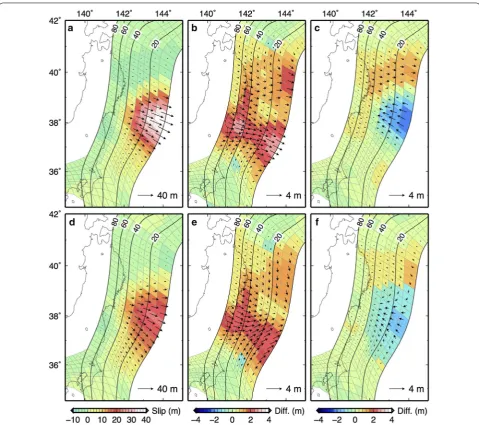
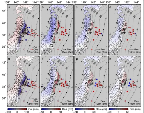
Results for slip inversions with the different elastic structures are shown in Fig. 7. Upper panels (Fig. 7a–c) show results using both onshore and offshore data, and lower panels (Fig. 7d–f) for results using only onshore data. Figure 7a, d shows inversion results for HOM. Fig-ure 7b, e shows slip vectors of LYR subtracting HOM slip, and Fig. 7c, f shows SLAB subtracting LYR. Calculated surface displacements are shown in Fig. 8. Upper pan-els show results using both onshore and offshore data, and lower panels for results using only onshore data. Figure 8a, e shows comparison of the calculated and observed displacements for HOM. Figure 8b, f shows residual (observed minus computed) displacements for HOM, Fig. 8c, g for LYR, and Fig. 8d, h for SLAB. Param-eters for slip distribution and data fitting in each case are summarized in Table 1.
Page 8 of 15 Hashima et al. Earth, Planets and Space (2016) 68:159
magnitude of 9.04. In the SLAB case, the maximum slip drops to 37.3 m, while the seismic moment and the moment magnitude further increase to 7.16 × 10²² Nm and 9.17, respectively. We can see a local slip increase area at 40°N (Fig. 7c). This increase appears to cancel out the negative dip slip seen for HOM (Figs. 6a, 7a). The increase in seismic moment from HOM, to LYR, to SLAB mostly reflects the increase in rigidity in the surround-ing material. Potency is more appropriate for compari-sons of slip characteristics (e.g., Ampuero and Dahlen
2005; Hearn and Bürgmann 2005) and increases from 1.06 × 10¹² m3 (HOM) to 1.18 × 10¹² m3 (LYR) and then drops slightly to 1.16 × 10¹² m3 (SLAB) as does the maxi-mum slip (Table 1). The residual displacements (Fig. 8b– d) decrease in both horizontal and vertical components, and at both onshore and offshore stations, indicating an improvement of fit using SLAB or LYR compared to the HOM case. Looking at the residuals in detail, the decrease in residual occurs more to the south at 37–38°N
at the HOM → LYR step (Fig. 8b, c), and the remaining residual at ~40°N diminishes for the LYR → SLAB step (Fig. 8c, d). These changes appear related to the move-ment of the area of slip change from ~37°N (Fig. 7b) to ~38°N (Fig. 7c). In terms of variance reduction, the layer-ing effect is dominant in improvlayer-ing the HOM model, but the slab also contributes to an improvement (Table 1).
Results for the onshore only inversion show simi-lar features to those for the full inversion. Compared to the results for the combined inversion, the slip in HOM is more broadly distributed, and the maximum slip decreases to 22.4 m, which is consistent with other stud-ies without offshore data (Ozawa et al. 2011; Iinuma et al.
2011). The maximum slip slightly increases to 23.2 m in LYR and then decreases to 22 m in SLAB model. Potency shows a similar trend, from 0.95 × 10¹² m3 (HOM) to 1 × 10¹² m3 (LYR) and 0.97 × 10¹² m3 (SLAB) The seismic moment increases steadily from 3.31 × 10²² Nm (HOM), through 4.01 × 10²² Nm (LYR), to 6.07 × 10²² Nm
(SLAB), as expected from the background modulus increase. Seismic moment and potency in each structure are slightly smaller than those obtained in the combined inversion. These decreases are consistent with the find-ings of Diao et al. (2012) and Kyriakopoulos et al. (2013). Variance reduction generally indicates a better fit in each case compared to the corresponding combined inversion case. The offshore data are difficult to fit because they are biased by spatial sparseness, even for our weighting choices, and may include preseismic and postseismic deformation (Sato et al. 2011).
An interesting feature of these results is the increase and decrease in the maximum slip and potency from HOM to SLAB. We may understand these results by con-sidering the layering and interface effects. In slip inver-sions, the layering effect requires larger slip given the increase in the average rigidity for the same surface dis-placements, and the interface effect requires smaller slip with the stronger footwall for the same surface displace-ments. A balance of these two effects controls the effect of the elastic structure on slip inversions. Comparing the layering and slab effects in slip inversions, the relative importance of the layering displacements is, naturally, larger for the purely layered case, and the relative impor-tance of the interface displacements is larger in the slab case (Fig. 4). This would explain the increase in the maxi-mum slip for LYR and their decrease compared to SLAB.
As we have seen, the offshore displacements are impor-tant for accounting for the effect of elastic structure close to the interface. One might expect that the maximum slip (and potency) would increase at LYR → SLAB step without offshore data, because mainly the layering effect contributes. To the contrary, the result shows the maxi-mum slip decreases for the combined inversion case. This contradiction can be understood by observing the verti-cal component. The vertiverti-cal deformation can be more effective when we do not use the offshore data, because it is more localized in the closer (east) side of the land. From Fig. 4b, c, the change in the vertical displacement at HOM → LYR and LYR → SLAB steps is reversed in sign with the former characterized by decrease in sub-sidence (relative uplift), and the latter is characterized by the weak increase in subsidence (relative subsidence), though the relative subsidence area is placed more on north. Thus, to fit the data requires slip increase in LYR and slip decrease in SLAB. Given our results on the role of the Poisson’s ratio, however, such subtle effects in the verticals may not be robust.
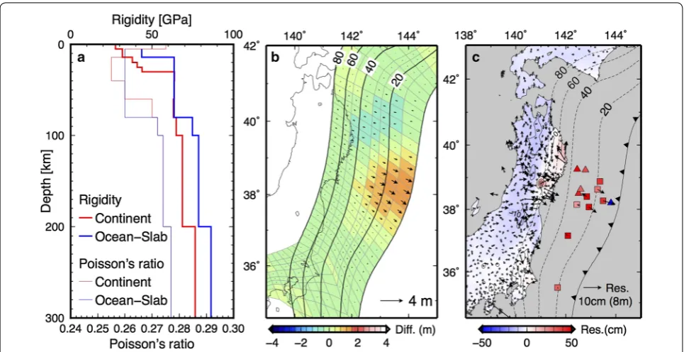
We examined three basic models to understand the basic behavior with changes in the overall elastic struc-ture. Studies of seismic tomography, for example, indi-cate seismic velocity heterogeneity on smaller scales. We therefore further consider if an improvement in data fit can be achieved with possibly more realistic elastic struc-ture. We take 1-D averaged vertical structure under Japan from seismic tomography (Matsubara et al. 2008) and elastic structure of the oceanic lithosphere from Miura et al. (2005). Mantle structure under the oceanic side is assumed to be the same as the continental sides. PAC and PHS slabs under the depth of 80 km are assumed to have 5 % larger seismic velocities than the surrounding mantle (Fig. 9a).
Figure 9 shows the inversion results. The overall slip distribution is similar to Figs. 6a and 7a. Compared Fig. 6 Test results for inversion uncertainties and the effect of the
Page 10 of 15 Hashima et al. Earth, Planets and Space (2016) 68:159
to SLAB, the maximum slip increases from 37.3 to 38.7 m and the potency increases from 1.16 × 10¹² to 1.18 × 10¹² m3. On the other hand, seismic moment decreases from 7.16 × 10²² to 5.61 × 10²² Nm. These changes can be explained by the decrease in the inter-face effect due to the introduction of the weak oceanic crust. The residual pattern of data fit (Fig. 9c) is similar to SLAB, but the overall variance reduction reduced from 0.9981 to 0.9978. The slightly worse fit of the more “real-istic” model may be due to a bias arising from the appli-cation of regional 3-D continental and oceanic velocity structures to our layered model structure and is likely not a comprehensive test of other 3-D heterogeneity.
However, this experiment serves to illustrate robustness of our results.
One might also be interested in effects of elastic struc-tures on coseismic stress change. However, given our simplified elastic structures with little lateral heteroge-neity, we find very little difference for shallow stress in terms of both amplitude and style of the stress tensor throughout the domain.
Discussion
Fig. 8 Calculated displacements from inverted slip for HOM and residual from observed data. Horizontal components are indicated by arrows, and vertical components are indicated by color. Contour for vertical components is taken at a, e 20-cm and b–d, f–h 10-cm intervals. Offshore stations are indicated by triangles and squares. Panels a–d for results using both onshore and offshore data. Panels e–h for results using only onshore data. a, e Calculated displacements for HOM together with observed displacements. b, f Residuals (observed displacements minus calculated displace-ments) for HOM model. c, g Residuals for LYR. d, h Residuals for SLAB. Solid line with triangles shows trench. Dashed lines show PAC slab contours
Table 1 Parameters for slip distribution and variance reduction (VR) in different elastic structures
VR for horizontal and vertical components and for the onshore and offshore regions are also shown. Structure name without and with star indicates inversion results using both onshore and offshore data and using only onshore data, respectively
HOM LYR SLAB HOM* LYR* SLAB*
Maximum slip (m) 38.5 39.6 37.3 22.4 23.2 22.0
Potency (1012 m3) 1.06 1.18 1.16 0.95 1.00 0.97
Moment (1022 Nm) 3.72 4.49 7.16 3.31 4.01 6.07
Magnitude 8.98 9.04 9.17 8.95 9.00 9.12
VR 0.9956 0.9973 0.9981 0.9988 0.9993 0.9994
VR (horizontal) 0.9968 0.9979 0.9985 0.9992 0.9995 0.9995
VR (vertical) 0.4240 0.7290 0.7901 0.6262 0.8372 0.8620
VR (onshore) 0.9985 0.9991 0.9993 0.9988 0.9993 0.9994
Page 12 of 15 Hashima et al. Earth, Planets and Space (2016) 68:159
elastic heterogeneity have been published already. For the layering effects, our results are consistent with an increase in the seismic moment, but not consistent in terms of increasing the maximum slip (Pollitz et al. 2011; Diao et al. 2012; Dong et al. 2014). This is likely because we adopted a stronger smoothing constraint on the slip distribution, adjusting the damping based on consistent trade-off curve analysis. However, the bulk parameter seismic potency is a more robust measure to assess the elastic effect.
As for the slab effect, our results do not indicate a sig-nificant role of contrasts in rigidity across the plate inter-face compared to crust–mantle layering. Instead, fitting in the onshore region also plays an important role. This result conflicts with Kyriakopoulos et al. (2013), who emphasized its importance. One of the reasons for this mismatch might stem from the elastic contrast used. The rigidity ratio in our SLAB model is 2.4, while Kyri-akopoulos et al.’s (2013) model used 3.7. According to studies of seismic tomography (e.g., Nakajima et al. 2001; Huang et al. 2011), velocity anomalies (VP and VS) in the slab compared to the surrounding mantle are ~6 %, implying that even our contrast might be on the high end. Kyriakopoulos et al.’s (2013) larger contrast may lead to an overestimate of the effect of elastic heterogeneity. Their elastic contrast also leads to poor fit of the vertical
displacements (Fig. 4c in Kyriakopoulos et al. 2013). Additionally, their choice of large Poisson’s ratio of 0.34 for continental crust may also cause an underestimate of vertical displacements (Fig. 5h). Studies of seismic tomography do not support VP/VS ratios corresponding to such a high Poisson’s ratio except in the toe part of the overriding plate (Matsubara and Obara 2011; Yamamoto et al. 2014).
comprehensive understanding might be possible based on the two effects. Conversely, incompleteness of data, such as lack of the offshore data, may lead to difficulty in inferring the individual elastic effects.
In this study, the SLAB model shows the best data fit (Table 1). Still, we can see systematic residuals (Fig. 8d). Most notably, vertical residuals are positive on the east coast and negative in the west coast. This broad anom-aly might reflect regional elastic heterogeneity, in par-ticular of Poisson’s ratio, with distance from the trench to the back-arc. Alternatively, the crustal thickness may gradually thin westward, or it could be attributed to the existence of an oceanic crust in the Sea of Japan and the thinned crust in the Miocene back-arc rift basin along the west coast (Matsubara et al. 2008). In this study, we did not consider lateral changes in crustal thickness, but such complexities would be straightforward to imple-ment, and we expect that the misfit would be further reduced. We can also see a large positive vertical residual at (141°E, 39°N). This could be because of the local sub-sidence due to the hot material under a nearby volcano (Takada and Fukushima 2013), though the volcano itself is located slightly to the west.
Systematic horizontal residual vectors are also found in Fig. 8d. Westward-oriented residuals are found along the west coast and northward residuals on both sides of the strait at 41.5°N, which are also found in previous stud-ies (Iinuma et al. 2012; Perfettini and Avouac 2014). The residuals along the west coast might be related to the thin oceanic crust of the Sea of Japan and the Miocene back-arc rift basin. The northward residuals around the strait might reflect some regional tectonics around the corner of the plate boundary zone between the northeast Japan and Kuril arcs. More strongly localized residuals on the east coast may be related to local elastic heterogeneities in the crust (Ohzono et al. 2012).
Conclusions
We investigated effects of elastic structure on coseismic deformation due to the 2011 Tohoku-oki earthquake, Japan, with a 3-D finite element model with forward and inverse approaches. We observed two main effects of het-erogeneity for fixed slip tests: (1) On large spatial scales, elastic layering leads to a decrease in surface displace-ment with an increase in the average rigidity. (2) Close to the slab interface, surface displacements increase with the increase in rigidity across the fault. Both layered structure and slab effects are expressed as the superposi-tion of the layering and interface effects. We also found that the vertical displacement modification due to slab structure was sensitive to the Poisson’s ratio of the con-tinental crust.
When the heterogeneous models are employed in inversions, the maximum slip increases from 38.5 m in the homogeneous to 39.6 m in the layered case and decreases to 37.3 m when slabs are introduced, and potency changes accordingly. While only of order 5–10 % of the maximum slip, patterns of local slip modification are robust, and the rheologically more realistic models do provide a better fit to the data. Inclusion of slip on the Philippine Sea plate interface has little impact. Further improvements of data fit may therefore be possible by introducing local heterogeneity near the surface and local topography.
Among the elastic heterogeneity effects, layering has the larger impact on inferred slip and leads to a broader and deeper slip patch compared to the homogeneous model, particularly to the south of the overall slip maxi-mum. The further introduction of a strong slab leads to a reduction in slip around the maximum slip and a slight increase further toward the north, both effects localized close to the trench. While heterogeneity is thus of minor importance for bulk properties such as potency, a lay-ered medium with a slab shows a systematically modified response, and the inferred differences in slip distribution may matter for detailed regional effects, such as infer-ences on afterslip or viscoelastic relaxation.
Abbreviations
PHS: Philippine Sea plate; EUR: Eurasian plate; PAC: Pacific plate; HOM: homo-geneous structure; LYR: layered structure; SLAB: slab structure.
Authors’ contributions
AH explored the elastic effects, performed the computations, and prepared the manuscript. TWB contributed to the inversion results, their interpretation, and study design. AH and AMF made the finite element model. HS provided the structural data for constructing the finite element model. AH and DAO made the model of plate boundaries. All authors read and approved the final manuscript.
Author details
1 Earthquake Research Institute, University of Tokyo, Yayoi 1-1-1, Bunkyo-ku,
Tokyo 113-0032, Japan. 2 Department of Earth Sciences, University of
South-ern California, Los Angeles, CA, USA. 3 Present Address: Jackson School
of Geosciences, The University of Texas at Austin, Austin, TX, USA. 4
Depart-ment of Earth, Atmospheric, and Planetary Sciences, Purdue University, West Lafayette, IN, USA.
Acknowledgements
Page 14 of 15 Hashima et al. Earth, Planets and Space (2016) 68:159
Competing interests
The authors declare that they have no competing interests.
Appendix: Expression for the roughness matrix The roughness matrix L is constructed with the discre-tized Laplace operator for strike and dip slip components as described below. We may approximate the Laplace operator for slip element xi at the center of patch i using distance to the surrounding patch centers rik in the form,
where C is the normalizing constant, r´i is the average dis-tance to the surrounding patches, n is the number of the surrounding patches and m is the geometric constant. C and r¯i are written as
n and m take the different values with respect to loca-tion in the source region: n = 6 and m = 4 for the patches inside, n = 5 and m = 3 for the patches on the edge, and n = 3 and m = 2 for the corner patches. Note that we use only 6 patches from 8 neighboring patches and likewise for edge patches, considering that the alignment of the patches is generally oblique and twisted. Then, explicit expression for Lij is as follows,
Received: 3 June 2016 Accepted: 14 September 2016
References
Ampuero J-P, Dahlen FA (2005) Ambiguity of the moment tensor. Bull Seismol Soc Am 95:390–400
Baba T, Tanioka Y, Cummins PR, Uhira K (2002) The slip distribution of the 1946 Nankai earthquake estimated from tsunami inversion using a new plate model. Phys Earth Planet Inter 132:59–73
Diao FQ, Xiong X, Zheng Y (2012) Static slip model of the Mw 9.0 Tohoku (Japan) earthquake: results from joint inversion of terrestrial GPS data and seafloor GPS/acoustic data. Chin Sci Bull 57:1990–1997
Dong J, Sun W, Zhou X, Wang R (2014) Effects of Earth’s layered structure, grav-ity and curvature on coseismic deformation. Geophys J Int 199:1442– 1451. doi:10.1093/gji/ggu342
Fujii Y, Satake K, Sakai S, Shinohara M, Kanazawa T (2011) Tsunami source of the 2011 off the Pacific coast of Tohoku Earthquake. Earth Planets Space 63:815–820
Hayes GP, Wald DJ, Johnson RL (2012) Slab1.0: a three-dimensional model of global subduction zone geometries. J Geophys Res 117:B01302. doi:10.1 029/2011JB008524
Hearn E, Bürgmann R (2005) The effect of elastic layering on inversions of GPS data for coseismic slip and resulting stress changes: strike-slip earth-quakes. Bull Seismol Soc Am 95:1637–1653
Hino R, Ito Y, Suzuki K, Suzuki S, Inazu D, Iinuma T, Ohta Y, Fujimoto H, Shino-hara M, Kaneda Y (2011) Foreshocks and mainshock of the 2011 Tohoku Earthquake observed by ocean bottom seismic/geodetic monitoring. Abstract of AGU 2011 Fall Meeting U51B-0008
Hirose F, Nakajima J, Hasegawa A (2008a) Three-dimensional seismic velocity structure and configuration of the Philippine Sea slab in southwestern Japan estimated by double-difference tomography. J Geophys Res 113:B09315. doi:10.1029/2007JB005274
Hirose F, Nakajima J, Hasegawa A (2008b) Three-dimensional velocity structure and configuration of the Philippine Sea slab beneath Kanto district, central Japan, estimated by double-difference tomography (in Japanese with English abstract). J Seismol Soc Jpn 60:123–138
Hsu Y-J, Simons M, Williams C, Casarotti E (2011) Three-dimensional FEM derived elastic Green’s functions for the coseismic deformation of the 2005 Mw 8.7 Nias-Simeulue, Sumatra earthquake. Geochem Geophys Geosyst 12:Q07013. doi:10.1029/2011GC003553
Huang Z, Zhao D, Wang L (2011) Seismic heterogeneity and anisotropy of the Honshu arc from the Japan Trench to the Japan Sea. Geophys J Int 184:1428–1444
Iinuma T, Ohzono M, Ohta Y, Miura S (2011) Coseismic slip distribution of the 2011 off the Pacific coast of Tohoku Earthquake (M 9.0) estimated based on GPS data—Was the asperity in Miyagi-oki ruptured? Earth Planets Space 63:643–648
Iinuma T, Hino R, Kido M, Inazu D, Osada Y, Ito Y, Ohzono M, Tsushima H, Suzuki S, Fujimoto H, Miura S (2012) Coseismic slip distribution of the 2011 off the Pacific Coast of Tohoku Earthquake (M9.0) refined by means of seafloor geodetic data. J Geophys Res 117:B07409. doi:10.1029/201 2JB009186
Ishibe T, Shimazaki K, Satake K, Tsuruoka H (2011) Change in seismicity beneath the Tokyo metropolitan area due to the 2011 off the Pacific coast of Tohoku Earthquake. Earth Planets Space 63:731–735
Ito Y, Tsuji T, Osada Y, Kido M, Inazu D, Hayashi Y, Tsushima H, Hino R, Fujimoto H (2011) Frontal wedge deformation near the source region of the 2011 Tohoku-Oki earthquake. Geophys Res Lett 38:L00G05. doi:10.1029/201 1GL048355
Kido M, Osada Y, Fujimoto H, Hino R, Ito Y (2011) Trench-normal variation in observed seafloor displacements associated with the 2011 Tohoku-Oki earthquake. Geophys Res Lett 38:L24303. doi:10.1029/2011GL050057 Kita S, Okada T, Hasegawa A, Nakajima J, Matsuzawa T (2010) Anomalous
deepening of a seismic belt in the upper-plane of the double seismic zone in the Pacific slab beneath the Hokkaido corner: possible evidence for thermal shielding caused by subducted forearc crust materials. Earth Planet Sci Lett 290:415–426
Kyriakopoulos C, Masterlark T, Stramondo S, Chini M, Bignami C (2013) Coseis-mic slip distribution for the Mw 9 2011 Tohoku-Oki earthquake derived from 3-D FE modeling. J Geophys Res 118:3837–3847
Maeda T, Furumura T, Sakai S, Shinohara S (2011) Significant tsunami observed at ocean-bottom pressure gauges during the 2011 off the Pacific coast of Tohoku Earthquake. Earth Planets Space 63:803–808
Matsubara M, Obara K (2011) The 2011 off the Pacific coast of Tohoku Earth-quake related to a strong velocity gradient with the Pacific plate. Earth Planets Space 63:663–667
Matsubara M, Obara K, Kasahara K (2008) Three-dimensional P- and S-wave velocity structures beneath the Japan Islands obtained by high-density seismic stations by seismic tomography. Tectonophysics 454:86–103 Menke W (2012) Geophysical data analysis: discrete inverse theory, MATLAB
edn (3rd edn). Academic Press (Elsevier), Waltham
Miura S, Takahashi N, Nakanishi A, Tsuru T, Kodaira S, Kaneda Y (2005) Structural characteristics off Miyagi forearc region, the Japan Trench seismogenic zone, deduced from a wide-angle reflection and refraction study. Tec-tonophysics 407:165–188
Nakajima J, Hasegawa A (2006) Anomalous low-velocity zone and linear alignment of seismicity along it in the subducted Pacific slab beneath Kanto, Japan: reactivation of subducted fracture zone? Geophys Res Lett 33:L16309. doi:10.1029/2006GL026773
Nakajima J, Matsuzawa T, Hasegawa A, Zhao D (2001) Three-dimensional struc-ture of Vp, Vs, and Vp/Vs beneath northeastern Japan: implications for arc magmatism and fluids. J Geophys Res 106:21843–21857
Nakajima J, Hirose F, Hasegawa A (2009) Seismotectonics beneath the Tokyo metropolitan area, Japan: effect of slab-slab contact and overlap on seismicity. J Geophys Res 114:B08309. doi:10.1029/2008JB006101 Nishimura T, Munekane H, Yarai H (2011) The 2011 off the Pacific coast of
Tohoku Earthquake and its aftershocks observed by GEONET. Earth Planets Space 63:631–636
Ohzono M, Yabe Y, Iinuma T, Ohta Y, Miura S, Tachibana K, Sato T, Demachi T (2012) Strain anomalies induced by the 2011 Tohoku Earthquake (Mw 9.0) as observed by a dense GPS network in northeastern Japan. Earth Planets Space 64:1231–1238
Ozawa S, Nishimura T, Suito H, Kobayashi T, Tobita M, Imakiire T (2011) Coseismic and postseismic slip of the 2011 magnitude-9 Tohoku-Oki earthquake. Nature 475:373–376
Ozawa S, Nishimura T, Munekane H, Suito H, Kobayashi T, Tobita M, Imakiire T (2012) Preceding, coseismic, and postseismic slips of the 2011 Tohoku earthquake, Japan. J Geophys Res 117:B07404. doi:10.1029/2011JB009120 Perfettini H, Avouac JP (2014) The seismic cycle in the area of the 2011 Mw9.0
Tohoku-Oki earthquake. J Geophys Res 119:4469–4515. doi:10.1002/201 3JB010697
Pollitz FF, Bürgmann R, Banerjee P (2011) Geodetic slip model of the 2011 M9.0 Tohoku earthquake. Geophys Res Lett 38:L00G08. doi:10.1029/201 1GL048632
Pulvirenti F, Jin S, Aloisi M (2014) An adjoint-based FEM optimization of coseismic displacements following the 2011 Tohoku earthquake: new insights for the limits of the upper plate rebound. Phys Earth Planet Inter 237:25–39
Romano F, Trasatti E, Lorito S, Piromallo C, Piatanesi A, Ito Y, Zhao D, Hirata K, Lanucara P, Cocco M (2014) Structural control on the Tohoku earthquake rupture process investigated by 3D FEM, tsunami and geodetic data. Sci Rep 4:5631. doi:10.1038/srep05631
Sagiya T, Miyazaki S, Tada T (2000) Continuous GPS array and present-day crustal deformation of Japan. Pure appl Geophys 157:2303–2322 Sato M, Ishikawa T, Ujihara N, Yoshida S, Fujita M, Mochizuki M, Asada A (2011)
Displacement above the hypocenter of the 2011 Tohoku-oki earthquake. Science 332:1395
Smith WHF, Wessel P (1990) Gridding with continuous curvature splines in tension. Geophysics 55:293–305
Suzuki W, Aoi S, Sekiguchi H, Kunugi T (2011) Rupture process of the 2011 Tohoku-Oki mega-thrust earthquake (M9.0) inverted from strong motion data. Geophys Res Lett 38:L00G16. doi:10.1029/2011GL049136 Takada Y, Fukushima Y (2013) Volcanic subsidence triggered by the 2011
Tohoku earthquake in Japan. Nature Geosci 6:637–641
Wessel P, Smith WHF (1998) New, improved version of the generic mapping tools released. EOS Trans AGU 79:579
Yagi Y, Fukahata Y (2011) Rupture process of the 2011 Tohoku-oki earthquake and absolute elastic strain release. Geophys Res Lett 38:L19307. doi:10.10 29/2011GL048701