Robust Adaptive Time Delay Estimation for Speaker
Localization in Noisy and Reverberant
Acoustic Environments
Simon Doclo
Department of Electrical Engineering, Katholieke Universiteit Leuven, ESAT-SISTA, Kasteelpark Arenberg 10, B-3001 Heverlee, Belgium
Email:[email protected]
Marc Moonen
Department of Electrical Engineering, Katholieke Universiteit Leuven, ESAT-SISTA, Kasteelpark Arenberg 10, B-3001 Heverlee, Belgium
Email:[email protected]
Received 23 September 2002 and in revised form 2 June 2003
Two adaptive algorithms are presented for robust time delay estimation (TDE) in acoustic environments with a large amount of background noise and reverberation. Recently, an adaptive eigenvalue decomposition (EVD) algorithm has been developed for TDE in highly reverberant acoustic environments. In this paper, we extend the adaptive EVD algorithm to noisy and reverber-ant acoustic environments, by deriving an adaptive stochastic gradient algorithm for the generalized eigenvalue decomposition (GEVD) or by prewhitening the noisy microphone signals. We have performed simulations using a localized and a diffuse noise source for several SNRs, showing that the time delays can be estimated more accurately using the adaptive GEVD algorithm than using the adaptive EVD algorithm. In addition, we have analyzed the sensitivity of the adaptive GEVD algorithm with respect to the accuracy of the noise correlation matrix estimate, showing that its performance may be quite sensitive, especially for low SNR scenarios.
Keywords and phrases:time delay estimation, acoustic source localization, generalized eigenvalue decomposition, stochastic gradient.
1. INTRODUCTION
In many speech communication applications, such as tele-conferencing, hand-free voice-controlled systems, and hear-ing aids, it is desirable to localize the dominant speaker. By using a microphone array, it is possible to determine the po-sition of this speaker such that the microphone array can be electronically steered using a fixed (or adaptive) beam-former in order to provide spatially selective speech acquisi-tion [1,2]. In multimedia teleconferencing systems, the po-sition of the speaker can be used not only for microphone array beamforming, but also for automatic video camera steering [3,4] and for determining binaural cues for stereo imaging.
It has been shown that it is possible to calculate the po-sition of a speaker from thetime delaysbetween the different microphone signals, for example, using maximum likelihood or least-squares methods [5,6]. However, accurate estima-tion of the time delays between the different microphone sig-nals is not an easy task because of the room reverberation, the
acoustic background noise, and the nonstationary character of the speech signal. Generally, room reverberation is consid-ered to be the main problem for time delay estimation (TDE) [7], but acoustic background noise can also considerably de-crease the performance of TDE algorithms. Whereas highly noisy situations are not very common in typical teleconfer-encing applications, they frequently occur in, for example, hearing aid applications.
(EVD) algorithm has been developed for (partial) estima-tion of twoacoustic impulse responsesusing a stochastic gra-dient algorithm that iteratively estimates the eigenvector cor-responding to the smallest eigenvalue. From the estimated acoustic impulse responses, the time delay can be calcu-lated as the time difference between the main peak (di-rect path) of the two impulse responses or as the peak of the correlation function between the two impulse responses. Since only the time difference between the main peak (di-rect path) of the impulse responses is required, it is there-fore not necessary to estimate the complete acoustic impulse responses.
The adaptive EVD algorithm for TDE performs much better in highly reverberant environments than the GCC-based methods. However, the adaptive EVD algorithm is— strictly speaking—only valid if either no noise or if spa-tiotemporally white noise is present. In this paper, we extend the adaptive EVD algorithm for TDE to the spatiotemporally colored noise case by using an adaptive generalized eigen-value decomposition (GEVD) algorithm or by prewhitening the noisy microphone signals. Furthermore, we extend all considered TDE algorithms to the case of more than two mi-crophones.
The paper is organized as follows.Section 2discusses the batch, that is, nonadaptive estimation of the complete acous-tic impulse responses from the recorded microphone signals. It is shown that if the length of the impulse responses is ei-ther known or can be overestimated, the complete impulse responses can be identified from the EVD of the speech cor-relation matrix (noiseless case and spatiotemporally white noise case) or from the GEVD of the speech and the noise correlation matrices (colored noise case). These batch im-pulse response estimation procedures form the basis for de-riving stochastic gradient algorithms that iteratively estimate the (generalized) eigenvector corresponding to the smallest (generalized) eigenvalue. These adaptive EVD and GEVD algorithms are discussed in Section 3. In [12], it has been shown that the adaptive EVD algorithm can be used for TDE, remarkably, even when underestimating the length of the acoustic impulse responses. We will show that this re-sult also holds for the spatiotemporally colored noise case when using the adaptive GEVD algorithm (and the adaptive prewhitening algorithm) for TDE. In Section 4, it is shown that all considered batch and adaptive TDE algorithms can easily be extended to the case of more than two micro-phones. Section 5 describes the simulation results for dif-ferent reverberation conditions (ideal and realistic), differ-ent SNRs, and different noise sources (localized and diffuse noise source). For all conditions, it is shown that the time delays can be estimated more accurately using the adaptive GEVD algorithm and the adaptive prewhitening algorithm than using the adaptive EVD algorithm. Since the adaptive GEVD algorithm requires an estimate of the noise correla-tion matrix, we also analyze its sensitivity with respect to the accuracy of this noise correlation matrix estimate, show-ing that the performance of the adaptive GEVD algorithm may be quite sensitive to deviations, especially for low SNR scenarios.
2. BATCH ESTIMATION OF ACOUSTIC IMPULSE RESPONSES
This section discusses the nonadaptive estimation of the complete acoustic impulse responses from the recorded mi-crophone signals, for the noiseless case as well as for the spa-tiotemporally white and colored noise case. The techniques discussed in this section are based on the subspace method, for example, presented in [13,14] for different applications. We will briefly review these well-known techniques since they form the basis for deriving the stochastic gradient al-gorithms that iteratively estimate the (generalized) eigenvec-tor corresponding to the smallest (generalized) eigenvalue, which will be used for TDE in practice (seeSection 3).
ConsiderNmicrophones, where each microphone signal
yn[k], n=0, . . . ,N−1, at timek, consists of a filtered version
of the clean speech signals[k] and additive noise:
yn[k]=hn[k]⊗s[k] +vn[k]=xn[k] +vn[k], (1) wherexn[k] andvn[k] are the speech and the noise compo-nents received at thenth microphone, respectively,hn[k] is the acoustic impulse response between the speech source and thenth microphone, and⊗denotes convolution. The addi-tive noise can be colored and is assumed to be uncorrelated with the clean speech signal. The goal is to estimate the im-pulse responseshn[k] from the recorded microphone signals
yn[k] without any a priori knowledge about the clean speech
signals[k]. From the estimates of the complete acoustic im-pulse responses, it is then trivial to compute the time delays between the direct paths.
If we model the acoustic impulse responsehn[k] with an FIR-filterhnof lengthL, that is,
hn=hn[0] hn[1] · · · hn[L−1]T, (2) the relation
xTi,L[k]hj=xTj,L[k]hi, i, j=0, . . . ,N−1, (3) holds [12], with theL-dimensional data vector
xn,L[k]=xn[k] xn[k−1] · · · xn[k−L+ 1]
T (4)
sincehj[k]⊗xi[k]=hj[k]⊗hi[k]⊗s[k]=hi[k]⊗xj[k]. Although we do not explicitly attribute a time indexkto the impulse responses, this does not imply that they cannot be time variant. In the remainder of this section, we will assume
N=2, although all considered algorithms can be straightfor-wardly extended to the case of more than two microphones (seeSection 4).
2.1. Noiseless case
The (2K×2K)-dimensional correlation matrixRxKis defined as
RxK=
Rx11,K −Rx10,K
−Rx01,K Rx00,K
with the (K×K)-dimensional submatrix
Rxij,K =Ᏹxi,K[k]xTj,K[k], (6) andᏱ{·}denoting the expected value operator. IfK ≥ L, that is, when the true impulse response lengthLis overesti-mated, the correlation matrixRxK has rank K+L−1, and hence, its null space has dimensionK−L+ 1 under the con-dition that [15]
(1) the impulse responsesh0andh1do not have common
zeros;
(2) the ((K+L−1)×(K+L−1))-dimensional autocor-relation matrix of the clean speech signals[k] has full rank.
IfK =L, the null space ofRxK has dimension 1, and the 2L-dimensional vector
u=
h0 h1
(7)
belongs to this null space since, using (3),RxKu=0. Consider the EVD ofRxK,
RxK=Vx∆xVTx, (8) withVx a (2K×2K)-dimensional orthogonal matrix, con-taining the eigenvectors, and∆xa diagonal matrix, contain-ing the eigenvalues. Hence, the unit-norm eigenvector, corre-sponding to the only zero eigenvalue ofRxK, contains a scaled version of the two impulse responsesh0andh1.
IfK > L, the null space ofRxK is spanned byK−L+ 1 eigenvectors, corresponding to the K −L+ 1 zero eigen-values, which all contain a different filtered version of the impulse responses. By extracting the common part of the eigenvectors, which can be done, for example, by perform-ing a QR decomposition of the full null space or by usperform-ing a least squares approach [14], the correct impulse responses of lengthLcan be identified. IfK < L, the null space ofRxK is empty and the impulse responses cannot be correctly identi-fied.
2.2. Spatiotemporally white noise
If additive noise is present, we define the (2K × 2K )-dimensional speech correlation matrix RyK and the (2K × 2K)-dimensional noise correlation matrixRvK, similar to (5), as
RKy =
R11y,K −R10y,K −R01y,K R00y,K
,
RvK=
Rv11,K −Rv10,K
−Rv01,K Rv00,K
,
(9)
with the (K×K)-dimensional submatrices
Rij,Ky =Ᏹyi,K[k]yTj,K[k],
Rvij,K =Ᏹvi,K[k]vTj,K[k], (10)
and the K-dimensional vectorsyn,K[k] andvn,K[k] defined similarly as in (4). Assuming that the clean speech signals[k] and the noise components vn[k] are uncorrelated, we can write
RyK=RxK+RvK. (11) If the noise is spatiotemporally white, that is,RKv =σ2
vI, with
σ2
vthe noise power andIthe identity matrix, the impulse
re-sponses can be identified from the EVD of the speech corre-lation matrix
RyK=Vy∆yVTy. (12) In this case, we can write (12) using (8) and (11) as
RKy =Vx∆x+σv2IVTx, (13) such that Vy = Vx and∆y = ∆x +σv2I. If K = L, only
one of the diagonal elements of ∆y is equal toσ2
v (smallest
eigenvalue), and the eigenvector inVy, corresponding to this eigenvalue, again contains a scaled version of the impulse re-sponses. IfK > L, the procedure for estimating the impulse responses of lengthLis similar to the procedure in the noise-less case, now based on theK−L+ 1 eigenvectors inVy cor-responding to eigenvalues which are equal toσ2
v.
2.3. Spatiotemporally colored noise
If spatiotemporally colored noise is present, the acoustic im-pulse responses cannot be identified from the EVD of RyK, but they can still be identified from the GEVD ofRyKandRvK or from the EVD of the prewhitened speech correlation ma-trix. In both cases, the noise correlation matrixRvKneeds to be known in advance or we have to estimate it during noise-only periods, requiring the use of a voice activity detector which determines when speech is present.
(1) GEVD procedure. The GEVD ofRKy andRvK is defined as [16]
RyK=QΛyQT, RKv =QΛvQT, (14) withQa (2K×2K)-dimensional invertible, but not necessarily orthogonal, matrix, andΛyandΛv diago-nal matrices. From (11) and (14), it follows that
RvK−1RxK=RKv−1RKy −RvK =Q−TΛ−1
v Λy−IQT.
(15)
Since (RKv)−1Rx
K has rankK+L−1 (RvK is assumed
to be of full rank),K−L+ 1 diagonal elements of the diagonal matrixΛ−1
v Λyare equal to 1. Therefore,K−
L+ 1 columnsqofQ−Texist for which
contains a scaled version of the impulse responses. If
K > L, theK−L+ 1 vectorsqcontain different filtered versions of the impulse responses, and the procedure for estimating the correct impulse responses of length
Lis similar to the procedure in the noiseless case. (2) Prewhitening procedure. The (2K×2K)-dimensional
prewhitened speech correlation matrix ¯RKy is defined as
¯
RKy RvK−T/2RyKRvK−1/2, (17)
with (RvK)1/2 the (2K × 2K)-dimensional
(upper-triangular) Cholesky factor of the noise correlation matrixRvK, that is,RvK = (RvK)T/2(Rv
a scaled version of the impulse responses. IfK > L, the
K−L+ 1 vectors (RvK)−1/2u¯ contain different filtered
versions of the impulse responses, and the procedure for estimating the correct impulse responses of length
Lis similar to the procedure in the noiseless case.
It is readily verified that the GEVD procedure and the pre-whitening procedure are in fact equivalent since
¯
Λy=Λ−v1Λy, Q−T =RvK−1/2V¯y. (21)
However, the adaptive versions of both algorithms, which are presented in Section 3 and which will be used for TDE in practice, can produce different results.
2.4. Practical computation
In practice, we will not work with correlation matrices, but with data matrices. The (p×2K)-dimensional speech data matrixYK[k] is defined as
with p typically much larger thanK, such that the empir-ical speech correlation matrix can be computed as RKy = YTK[k]YK[k]/p. The noise data matrixVK[k] is defined simi-larly.
(1) GSVD procedure. Instead of computing the GEVD of RKy andRvK, we compute the generalized singular value decomposition (GSVD) of the data matrices YK[k] andVK[k], defined as
YK[k]=UyΣyQT, VK[k]=UvΣvQT, (23) withUyandUvorthogonal matrices,ΣyandΣv diag-onal matrices, andQa (2K×2K)-dimensional invert-ible, but not necessarily orthogonal, matrix [16,17]. Again, the impulse responses are estimated from the columnsqof the matrixQ−T.
(2) Prewhitening procedure. The prewhitened speech data matrix ¯YK[k] is defined as
¯
YK[k]=YK[k]RvK−1/2, (24) where the (2K×2K)-dimensional (upper-triangular) Cholesky factor (RvK)1/2can be computed using the QR
decomposition of the noise data matrix, that is,
VK[k]=QvRvK1/2. (25) The singular value decomposition (SVD) of ¯YK[k] is defined as
¯
YK[k]=U¯yΣ¯yV¯T
y, (26)
with ¯Uyand ¯Vy orthogonal matrices and ¯Σya diago-nal matrix. Again, the impulse responses are estimated from the columns ¯uof the matrix ¯Vy.
2.5. Simulation results
We have filtered a 16-kHz speech segment of 160000 samples (10 seconds) with 2 impulse responses (L = 20), which are depicted inFigure 1a. A stationary colored speech-like noise signal, having the same long-term spectrum as speech [18], has been added, and the SNR of the microphone signals is 10 dB.
−0.5 0 0.5 1
1 5 10 15 20
A
m
plitude
Filter taps
−0.5 0 0.5 1
1 5 10 15 20
A
m
plitude
Filter taps (a) Impulse responsesh0andh1.
−0.5 0 0.5 1
1 5 10 15 20
Am
p
li
tu
d
e
Filter taps
−0.5 0 0.5 1
1 5 10 15 20
Am
p
li
tu
d
e
Filter taps (b) Estimated impulse responses with SVD procedure.
−0.5 0 0.5 1
1 5 10 15 20
Am
p
li
tu
d
e
Filter taps
−0.5 0 0.5 1
1 5 10 15 20
Am
p
li
tu
d
e
Filter taps (c) Estimated impulse responses with GSVD procedure.
Figure1
3. ADAPTIVE PROCEDURE FOR TIME DELAY ESTIMATION
In practice, acoustic impulse responses may have thousands of taps,depending on the room reverberation. Because of the correlated nature of speech, correspondingly large autocor-relation matrices of the clean speech signals[k] can be rank deficient or at least ill conditioned [19]. Therefore, it is quite difficult to identify the complete impulse responses, espe-cially when a large amount of background noise is present [14]. If we underestimate the length of the impulse responses (K < L), the acoustic impulse responses estimated with the batch procedures are biased. This makes it difficult to cal-culate the correct time delays from these estimated acoustic impulse responses.
In [12], an adaptive EVD algorithm has been presented, which iteratively estimates the eigenvector corresponding to the smallest eigenvalue. Remarkably, even when underesti-mating the length of the impulse responses (K < L), simu-lations show that this adaptive EVD algorithm is still able to identify the main peak (direct path) of the impulse responses. Obviously, only the time difference between the main peak of the impulse responses is required for TDE.
the generalized eigenvector corresponding to the smallest generalized eigenvalue. Using simulations with spatiotem-porally colored noise, it will be shown that—just as for the adaptive EVD algorithm—it is possible to correctly estimate the time delays with the adaptive GEVD algorithm, even when underestimating the length of the acoustic impulse re-sponses (seeSection 5).
In the remainder of the text, we will assume that the length of the acoustic impulse responses is underestimated (K < L), and hence, we will derive algorithms that estimate the one-dimensional subspace corresponding to the smallest (generalized) eigenvalue.
3.1. Adaptive EVD algorithm [12]
Instead of updating the full EVD ofRKy [20] and then us-ing the eigenvector correspondus-ing to the smallest eigenvalue, it is possible to iteratively estimate this eigenvector by min-imizing the cost function uTRyKu subject to the constraint uTu=1. A cheap procedure consists in minimizing the mean square value of the error signale[k], defined as
e[k]=uT[k]yK[k]
u[k] , (27)
withyK[k] = yT1,K[k] −yT0,K[k]T. This expression in fact
is a Rayleigh quotient, whereλmax
y ≥Ᏹ{e2[k]} ≥λminy , with
λmax
y andλminy , respectively, the largest and the smallest
eigen-values of the correlation matrixRKy. Minimizing (27) can be done, for example, using a gradient-descent LMS procedure, where normalization is included in each iteration step in or-der to avoid roundofferror propagation [21],
u[k+ 1]= u[k]−µe[k]
∂e[k]/∂u[k] u[k]−µe[k]
∂e[k]/∂u[k], (28)
withµthe step size of the adaptive algorithm. The gradient ofe[k] is equal to
In [12], it has been assumed that the smallest eigenvalue of RKy is very small (in the noiseless case) such that the gradient eventually reduces to ∂e[k]/∂u[k] ≈yK[k], and the update
In [12], it has been indicated that a good initialization ofu and a proper choice of the parametersK andµare essential for a good convergence behavior. It has also been shown by simulations that the adaptive EVD algorithm performs more robustly in highly reverberant environments than the GCC-based methods.
3.2. Adaptive GEVD and prewhitening algorithm For the noise-robust GEVD and prewhitening procedures, described inSection 2.3, it is also possible to derive stochas-tic gradient algorithms which iteratively estimate the gen-eralized eigenvector corresponding to the smallest general-ized eigenvalue ofRKy andRvK. It will be assumed that the noise correlation matrix RvK (or its Cholesky factor) is ei-ther known or updated during noise-only periods. Since the noise correlation matrix cannot be updated during speech-and-noise periods, we have to assume that the noise is sta-tionary enough such that the noise correlation matrix com-puted during noise-only periods can be used in the up-date formulas during subsequent speech-and-noise peri-ods.
Adaptive GEVD algorithm
Instead of updating the full GEVD of RKy andRvK [22] and then using the generalized eigenvector corresponding to the smallest generalized eigenvalue, it is possible to iteratively es-timate this generalized eigenvector by minimizing the cost function qTRKyq subject to the constraint qTRvKq = 1. A cheap procedure consists in minimizing the mean square value of the error signal e[k], defined as the generalized Rayleigh quotient
which can be done, for example, using a gradient-descent LMS procedure
q[k+ 1]=q[k]−µe[k]∂e[k]
∂q[k], (32)
withµthe step size of the adaptive algorithm. The gradient ofe[k] now is equal to
such that, when taking mathematical expectation after con-vergence, we get
RKyq[∞]=Ᏹe2[k]Rv
Kq[∞]. (35)
simplify the expression in (34). In order to avoid roundoff error propagation, we include an additional normalization in each iteration step such that the update formulas can be written as
The prewhitening procedure can be made adaptive by using prewhitened speech data vectors ¯yK[k]=(RvK)−T/2y
K[k] in
the adaptive EVD procedure ofSection 3.1. The update for-mulas then become rithm) since the smallest eigenvalue of ¯RKy is not equal to zero (seeSection 2.3). The impulse response at timekis esti-mated as (RvK)−1/2u¯[k]. If the noise correlation matrixRv
Kis
not known in advance, the Cholesky factor (RvK)−1/2can be
updated by inverse QR updating during noise-only periods.
The computational complexity of the adaptive GEVD and the adaptive prewhitening algorithm is higher than that of the adaptive EVD algorithm since in each iteration step two additional matrix-vector multiplications (either with the noise correlation matrix or with the inverse Cholesky fac-tor) have to be performed. Reducing the computational com-plexity of these algorithms is a topic of further research. The noise correlation matrixRvKin the adaptive GEVD algorithm could be replaced, for example, by its instantaneous estimate v[k]vT[k], wherev[k] is a noise data vector which is stored in a buffer during noise-only periods and which is used in the update equations during subsequent speech-and-noise peri-ods. Similarly as in the momentum LMS algorithm [23], it could then also be advantageous to perform an averaging op-eration on (part of) the gradient∂e[k]/∂q[k].
In addition, the computational complexity of all pre-sented adaptive TDE algorithms can be reduced by using subsampling, that is, the estimated impulse response vectors are not updated for every time step at the expense of a slower convergence and tracking behavior.
4. EXTENSION TO MORE THAN TWO MICROPHONES
All presented (batch and adaptive) algorithms can easily be extended to the case of more than two microphones, either by constructing (p(N−1)×NK)-dimensional data matri-ces, considering the time delays between every microphone and the first microphone, or by constructing (pC2N×NK
)-dimensional data matrices (with C2
N all possible
combina-tions of two out ofN), considering the time delays between every combination of two microphones. For example, ifN= 3, the speech data matrixYK[k] in (22) can be redefined by
considering time delays between every microphone and the first microphone, or by the matrix
considering time delays between every combination of two microphones. The noise data matrix VK[k] is constructed similarly. It can easily be verified that, ifK =Land for the noiseless case, theNL-dimensional vector consisting of the impulse responses
belongs to the null space of the speech data matrix. There-fore all presented (batch and adaptive) algorithms can be used with the redefined data matrices and data vectors. For the adaptive algorithms, several updates now have to be per-formed in each iteration step, either withN−1 orC2
N data
vectors. However, the computational complexity can be re-duced, for example, by only performing an update with one data vector in each iteration step, that is, by using consecutive rows of the matrices (38) or (39) in each iteration step.
In [24], another adaptive algorithm has been proposed for extending these TDE procedures to more than two micro-phones. This algorithm is based on the minimization of an error signal constructed using all cross-correlations between the different microphone signals, either using a stochastic gradient (MCLMS) or a Newton (MCN) method, and re-quires only one update in each iteration step. It has been shown that this class of algorithms can be efficiently imple-mented in the frequency domain [25].
5. SIMULATIONS
A
m
plitude
−1
−0.5 0 0.5 1
Time (s)
0 1 2 3 4 5 6 7 8 9 10
(a) Clean speech signals[k].
A
m
plitude
−1
−0.5 0 0.5 1
Time (s)
0 1 2 3 4 5 6 7 8 9 10
(b) Noisy speech signaly0[k] (SNR=−5 dB).
Figure2
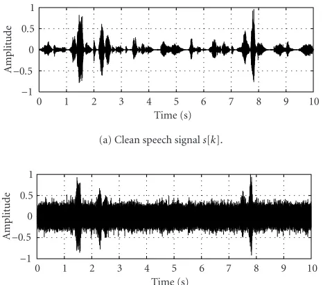
Figure 2a), such that no voice activity detector is required and we continuously estimate the time delays. For the sim-ulations in Sections5.1,5.2, and5.3, we have calculated the (exact) noise correlation matrix estimateRvK in advance us-ing the noise componentsvn[k], whereas, inSection 5.4, the sensitivity of the adaptive GEVD algorithm with respect to the accuracy of this noise correlation matrix estimate is an-alyzed. The time delay between the microphone signals is computed using the peak of the correlation function between the different estimated acoustic impulse responses.
5.1. No reverberation,N=2
In a first simulation, we have assumed no reverberation and
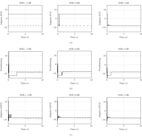
N = 2 microphones. We have used a colored noise sig-nal constructed by filtering white noise with the five-tap FIR filter [1 −4 6 4 0.5]. The microphone signals are con-structed such that the time delay between the speech com-ponents is−8 samples, whereas the time delay between the noise components is 5 samples. We have performed simula-tions using the adaptive EVD, prewhitening, and GEVD al-gorithms for different SNRs (−5 dB, 0 dB, 5 dB). The used filter lengthK =40, the subsampling factor for the update formulas is 10, and the step sizeµof the adaptive algorithms is chosen such that the optimal performance is obtained, that is, most of the estimated time delays are close to the correct time delay (in this case,µ=1e−7 for all algorithms).
Figure 3shows the TDE convergence plots for the diff er-ent adaptive algorithms for differer-ent SNRs. The correct time delay is indicated by the dashed line. As can be seen, the adaptive EVD algorithm converges to the correct time de-lay for SNR = 5 dB, but converges to the wrong time de-lay of the noise source for lower SNRs. Both the adaptive prewhitening and the adaptive GEVD algorithm converge to the correct time delay for all SNRs. The adaptive GEVD
algorithm converges faster than the adaptive prewhitening al-gorithm.
5.2. Realistic conditions,N=2
In order to simulate realistic reverberation conditions, we have simulated a room with dimensions 5m×4m×2m, hav-ing a reverberation timeT60 =250 milliseconds. The
rever-beration timeT60 can be expressed as a function of the
ab-sorption coefficientγof the walls, according to Eyring’s for-mula [26]
T60=
0.163V
−Slog(1−γ), (41)
withVthe volume of the room andSthe total surface of the room. The room consists of a microphone array, withN = 2 omnidirectional microphones at positions [1 1 1] and [1.5 1 1], and a speech source at position [2 2 1.7]. The speech componentsxn[k] received at the microphone array are filtered versions of the clean speech signal using simulated acoustic impulse responses, which are constructed using the image method [27,28] with a filter lengthL=1000.Figure 4 depicts the acoustic impulse responses h0[k] andh1[k] for
the speech source. The exact time delay between the speech components is−12.18 samples, which has been obtained by a simple geometrical calculation. We will perform simula-tions for a localized noise source at position [4 1.5 1] and for a diffuse, that is, isotropic, noise source. For the localized noise source, we have used a stationary colored speech-like noise signal having the same long-term spectrum as speech [18], and the noise componentsvn[k] received at the micro-phone array are filtered versions using simulated acoustic im-pulse responses. The diffuse noise source has been generated by considering 1000 uncorrelated white noise sources equally distributed over all directions.
We have performed simulations using the adaptive EVD, prewhitening, and GEVD algorithms for different SNRs (ranging from −10 dB to 10 dB) and for subsampling fac-tor 1, that is, no subsampling. The noisy microphone signal
y0[k] with SNR = −5 dB is plotted inFigure 2b. We have
usedK=40 and, for each algorithm, we have chosen the step sizeµwhich gives the best performance, that is the smallest percentage of anomalous estimates. An anomalous estimate is defined as a time delay estimate which corresponds to an angle outside a 5◦error region from the correct angle of in-cidence.
SNR=−5 dB
Figure3: TDE convergence plots of (a) adaptive EVD, (b) prewhitening, and (c) GEVD algorithms for different SNRs without reverberation (N=2,K=40, subsampling=10, andµ=1e−7).
algorithm converges to the correct time delay for SNR=0 dB without any knowledge of the noise characteristics.
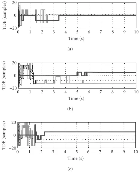
For the different adaptive TDE algorithms and for dif-ferent SNRs, Figure 7a shows the percentage of anomalous time delay estimates for the localized noise source, whereas Figure 7b shows the percentage of anomalous estimates for the diffuse noise source. As can be seen from both figures, the performance of the adaptive prewhitening and the adap-tive GEVD algorithms is better than the performance of the adaptive EVD algorithm for all scenarios. For the localized noise source, the performance of the adaptive EVD algorithm decreases dramatically when the SNR is smaller than 0 dB, whereas the performance of both the adaptive prewhitening
Am
p
li
tu
d
e
−1
−0.5 0 0.5 1
Taps
0 100 200 300 400 500 600 700 800 900 1000
(a) Speech impulse response of microphone 1.
Am
p
li
tu
d
e
−1
−0.5 0 0.5 1
Taps
0 100 200 300 400 500 600 700 800 900 1000
(b) Speech impulse response of microphone 2.
Figure4: Acoustic impulse responsesh0[k] andh1[k] for the speech
source.
TDE
(samples)
−20 0 20
0 1 2 3 4 5 6 7 8 9 10
Time (s) (a)
TDE
(samples)
−20 0 20
0 1 2 3 4 5 6 7 8 9 10
Time (s) (b)
TDE
(samples)
−20 0 20
0 1 2 3 4 5 6 7 8 9 10
Time (s) (c)
Figure5: TDE convergence plots of (a) adaptive EVD algorithm (µ=1e−3), (b) adaptive prewhitening algorithm (µ=1e−5), and (c) adaptive GEVD algorithm (µ=1e−3) withN =2,K =40, SNR= −5 dB,T60 =250 milliseconds, and subsampling=1. The
correct time delay is indicated by the dashed line.
TDE
(samples)
−20 0 20
0 1 2 3 4 5 6 7 8 9 10
Time (s) (a)
TDE
(samples)
−20 0 20
0 1 2 3 4 5 6 7 8 9 10
Time (s) (b)
TDE
(samples)
−20 0 20
0 1 2 3 4 5 6 7 8 9 10
Time (s) (c)
Figure6: TDE convergence plots of (a) adaptive EVD algorithm (µ=1e−3), (b) adaptive prewhitening algorithm (µ=1e−5), and (c) adaptive GEVD algorithm (µ=1e−3) withN =2,K =40, SNR = 0 dB,T60 = 250 milliseconds, and subsampling=1. The
correct time delay is indicated by the dashed line.
Instead of using the adaptive prewhitening or the adap-tive GEVD algorithm in highly noisy acoustic environments, it is also possible to first perform a noise reduction procedure as a preprocessing step for the adaptive EVD algorithm. We have considered two noise reduction algorithms.
(i) Aspectral subtraction(SS) technique on each micro-phone signal independently [29]. We have calculated the average noise spectrum for each microphone sig-nal in advance and have used a simple magnitude sub-traction weighting function [30] (FFT size=512, half-wave rectification, no noise overestimation, and no magnitude averaging).
(ii) A multichannel Wiener filtering (MWF) technique, making an optimal (MMSE) estimate of the speech components in each microphone signal using knowl-edge about the spatiotemporal correlation properties of the noise components. We have used a GSVD based implementation [31] with a filter length K = 40 on each microphone signal. Other implementations hav-ing a lower computational complexity, such as a sub-band implementation [32] or a QRD-based imple-mentation [33], could have also been used.
per-P
er
centage
anomalies
0 10 20 30 40 50 60 70 80 90 100
SNR (dB)
−10 −8 −6 −4 −2 0 2 4 6 8 10
EVD
EVD (preproc SS) EVD (preproc MWF)
Prewhitening GEVD
(a) Continuous speech—BLU noise.
P
er
centage
anomalies
0 5 10 15
SNR (dB)
−10 −8 −6 −4 −2 0 2 4 6 8 10
EVD
EVD (preproc SS) EVD (preproc MWF)
Prewhitening GEVD
(b) Continuous speech—diffuse noise.
Figure7: Percentage of anomalous estimates versus SNR for tive EVD (no preprocessing, SS and MWF preprocessing), adap-tive prewhitening, and adapadap-tive GEVD algorithms for (a) local-ized noise source and (b) diffuse noise source (N = 2,K =40, T60=250 milliseconds, and subsampling=1).
formance improvement, certainly for low SNR scenarios, whereas, for the diffuse noise source, the SS preprocessing apparently does not give rise to a performance improvement. For both the localized and the diffuse noise source, the MWF preprocessing reduces the percentage of anomalous estimates to below 1% for all SNRs. However, the computational com-plexity of the adaptive EVD algorithm combined with MWF preprocessing is still higher than the computational com-plexity of the adaptive GEVD algorithm.
TDE
(samples)
−20 0 20
0 1 2 3 4 5 6 7 8 9 10
Time (s) (a)
TDE
(samples)
−20 0 20
0 1 2 3 4 5 6 7 8 9 10
Time (s) (b)
TDE
(samples)
−20 0 20
0 1 2 3 4 5 6 7 8 9 10
Time (s) (c)
Figure8: TDE convergence plots of (a) adaptive EVD algorithm (µ=1e−3), (b) adaptive prewhitening algorithm (µ=1e−4), and (c) adaptive GEVD algorithm (µ=1e−2) withN =3,K =40, SNR= −5 dB,T60=250 milliseconds, and subsampling=10. The
TDE between microphones 1 and 2 is denoted by the solid line, the TDE between microphones 1 and 3 by the dotted line, and the TDE between microphones 2 and 3 by the thick solid line.
5.3. Realistic conditions,N=3
For the same acoustical conditions as inSection 5.2, we have performed simulations usingN=3 microphones, where the position of the third microphone is [1 1 1.5]. We have con-sidered the time delays between every combination of 2 mi-crophones and, in each iteration step, we have performed up-dates using all three data vectors from (39). The exact time delay between the speech components of the first and the sec-ond microphone signal is−12.18 samples, between the first and the third microphone signal−7.04 samples, and between the second and the third microphone signal 5.14 samples. We have performed simulations for different SNRs (−5 dB, 0 dB), the used filter lengthK =40, the subsampling factor is 10, and, for each algorithm, we have chosen the step sizeµ which gives rise to the best performance.
TDE
(samples)
−20 0 20
0 1 2 3 4 5 6 7 8 9 10
Time (s) (a)
TDE
(samples)
−20 0 20
0 1 2 3 4 5 6 7 8 9 10
Time (s) (b)
TDE
(samples)
−20 0 20
0 1 2 3 4 5 6 7 8 9 10
Time (s) (c)
Figure9: TDE convergence plots of (a) adaptive EVD algorithm (µ=1e−2), (b) adaptive prewhitening algorithm (µ=1e−4), and (c) adaptive GEVD algorithm (µ=1e−2) withN =3,K =40, SNR=0 dB,T60=250 milliseconds, and subsampling=10. The
TDE between microphones 1 and 2 is denoted by the solid line, the TDE between microphones 1 and 3 by the dotted line, and the TDE between microphones 2 and 3 by the thick solid line.
convergence plots for SNR=0 dB. In this case, all algorithms converge to the correct time delays, although the time delay between the second and the third microphone signal is only correctly estimated by the adaptive EVD algorithm in signal segments with a high segmental SNR.
From these simulations, we can conclude that, for all SNRs and microphone configurations, the adaptive prewhit-ening and the adaptive GEVD algorithms converge more ro-bustly to the correct time delays than the adaptive EVD algo-rithm, certainly in low SNR scenarios.
5.4. Sensitivity to the accuracy of the noise correlation matrix estimate
In the previous simulations, we have always assumed that an accurate estimate of the noise correlation matrixRvKis avail-able. Since it is well known that GEVD-based algorithms may be sensitive to the accuracy of this noise correlation matrix estimate, we will analyze the sensitivity of the adaptive GEVD algorithm in this section. Instead of using the (correct) noise correlation matrix estimateRvK, we will use
˜
RvK=RvK+αReK, (42)
P
er
centage
anomalies
0 10 20 30 40 50 60 70 80 90 100
Norm deviation of noise correlation matrix 1 1.5 2 2.5 3 3.5 4 4.5 5
SNR=−10 dB SNR=−5 dB SNR=0 dB
SNR=5 dB SNR=10 dB (a) Continuous speech—BLU noise (case 1).
P
er
centage
anomalies
0 10 20 30 40 50 60 70 80 90 100
Norm deviation of noise correlation matrix 1 1.5 2 2.5 3 3.5 4 4.5 5
SNR=−10 dB SNR=−5 dB SNR=0 dB
SNR=5 dB SNR=10 dB (b) Continuous speech—BLU noise (case 2).
Figure10: Sensitivity of adaptive GEVD algorithm with respect to noise correlation matrix estimate for (a) random deviation and (b) uncorrelated white noise deviation (localized noise source,N =2, K=40,T60=250 milliseconds, and subsampling=1).
withReK the deviation correlation matrix. We will consider two cases forReK:
(1) ReK is a random (symmetric) matrix corresponding to random errors on all correlation coefficients;
(2) ReKis equal to the identity matrix corresponding to un-correlated white noise on the microphones.
P
er
centage
anomalies
0 10 20 30 40 50 60 70 80 90 100
Norm deviation of noise correlation matrix 1 1.5 2 2.5 3 3.5 4 4.5 5
SNR=−10 dB SNR=−5 dB SNR=0 dB
SNR=5 dB SNR=10 dB (a) Continuous speech—diffuse noise (case 1).
P
er
centage
anomalies
0 1 2 3 4 5 6 7 8 9
Norm deviation of noise correlation matrix 1 1.5 2 2.5 3 3.5 4 4.5 5
SNR=−10 dB SNR=−5 dB SNR=0 dB
SNR=5 dB SNR=10 dB (b) Continuous speech—diffuse noise (case 2).
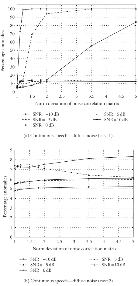
Figure11: Sensitivity of adaptive GEVD algorithm with respect to noise correlation matrix estimate for (a) random deviation and (b) uncorrelated white noise deviation (diffuse noise source,N = 2, K=40,T60=250 milliseconds, and subsampling=1).
β=R˜vK2 Rv
K2
. (43)
For the localized noise source,Figure 10ashows the sensitiv-ity of the adaptive GEVD algorithm for different SNRs when ReKis a random matrix, whereasFigure 10bshows the sensi-tivity whenReKis equal to the identity matrix. As can be seen, the adaptive GEVD algorithm is more sensitive to the accu-racy of the noise correlation matrix estimate for low SNR sce-narios and whenReKis a random matrix.
Figure 11shows the sensitivity of the adaptive GEVD al-gorithm for a diffuse noise source. As can be seen fromFigure 11a, whenReK is a random matrix, the sensitivity for a dif-fuse noise source is comparable to the sensitivity for a local-ized noise source. However, as can be seen fromFigure 11b, for a diffuse noise source, the adaptive GEVD algorithm is not very sensitive when ReK is equal to the identity matrix. This can be explained by the fact that, for a large microphone distance, the noise correlation matrixRvKfor a diffuse noise source is approximately equal to the identity matrix.
6. CONCLUSION
In this paper, we have presented two adaptive algorithms for robust TDE in adverse acoustic environments where a large amount of reverberation and additive noise is present. We have extended a recently developed adaptive EVD algorithm for TDE to noisy environments by using an adaptive GEVD or by prewhitening the microphone signals. For the adap-tive GEVD, we have derived a stochastic gradient algorithm which iteratively estimates the generalized eigenvector corre-sponding to the smallest generalized eigenvalue. In addition, we have extended all presented TDE algorithms to the case of more than two microphones. It has been shown by simula-tions that, for all considered scenarios, the time delays can be estimated more accurately using the adaptive prewhitening and the adaptive GEVD algorithms than using the adaptive EVD algorithm. However, the difference in performance be-tween the adaptive EVD and GEVD algorithms is negligible for SNRs higher than 5 dB and for a diffuse noise source, and the adaptive GEVD algorithm is quite sensitive to the accu-racy of the noise correlation matrix estimate for low SNR sce-narios.
ACKNOWLEDGMENTS
This work was carried out at the ESAT laboratory of the Katholieke Universiteit Leuven, and was sup-ported in part by the FWO Research Project G.0233.01, Signal Processing and Automatic Patient Fitting for Advanced Auditory Prostheses, the IWT Project 020540, Performance Improvement of Cochlear Implants by Innovative Speech Pro-cessing Algorithms, the IWT Project 020476, Sound Man-agement System for Public Address systems (SMS4PA), the Concerted Research Action,Mathematical Engineering Tech-niques for Information and Communication Systems (GOA-MEFISTO-666) of the Flemish Government, and the In-teruniversity Attraction Pole IUAP P5-22 (2002-2007), Dy-namical Systems and Control: Computation, Identification, and Modelling, initiated by the Belgian State, Prime Minis-ter’s Office, Federal Office for Scientific, Technical, and Cul-tural Affairs, and was partially sponsored by Cochlear. The authors would like to thank the reviewers for their valuable comments and suggestions.
REFERENCES
[2] S. Doclo and M. Moonen, “Design of broadband beamform-ers robust against gain and phase errors in the microphone array characteristics,” IEEE Trans. Signal Processing, vol. 51, no. 10, pp. 2511–2526, 2003.
[3] H. Wang and P. Chu, “Voice source localization for automatic camera pointing system in videoconferencing,” inProc. IEEE Int. Conf. Acoustics, Speech, Signal Processing, vol. 1, pp. 187– 190, Munich, Germany, April 1997.
[4] Y. Huang, J. Benesty, and G. W. Elko, “Microphone arrays for video camera steering,” inAcoustic Signal Processing for Telecommunication, S. L. Gay and J. Benesty, Eds., vol. 551 ofKluwer International Series in Engineering and Computer Science, chapter 11, pp. 239–259, Kluwer Academic Press, Boston, Mass, USA, March 2000.
[5] M. Wax and T. Kailath, “Optimum localization of multiple sources by passive arrays,” IEEE Trans. Acoustics, Speech, and Signal Processing, vol. 31, no. 5, pp. 1210–1218, 1983. [6] Y. Huang, J. Benesty, G. W. Elko, and R. M. Mersereau,
“Real-time passive source localization: a practical linear-correction least-squares approach,” IEEE Trans. Speech, and Audio Pro-cessing, vol. 9, no. 8, pp. 943–956, 2001.
[7] B. Champagne, S. B´edard, and A. St´ephenne, “Performance of time-delay estimation in the presence of room reverbera-tion,” IEEE Trans. Speech, and Audio Processing, vol. 4, no. 2, pp. 148–152, 1996.
[8] C. H. Knapp and G. C. Carter, “The generalized correlation method for estimation of time delay,” IEEE Trans. Acous-tics, Speech, and Signal Processing, vol. 24, no. 4, pp. 320–327, 1976.
[9] D. V. Rabinkin, R. J. Renomeron, A. J. Dahl, J. C. French, J. L. Flanagan, and M. H. Bianchi, “A DSP implementation of source location using microphone arrays,” inProc. SPIE, vol. 2846, pp. 88–99, Denver, Colo, USA, August 1996. [10] A. St´ephenne and B. Champagne, “A new cepstral prefiltering
technique for estimating time delay under reverberant condi-tions,”Signal Processing, vol. 59, no. 3, pp. 253–266, 1997. [11] P. C. Ching, Y. T. Chan, and K. C. Ho, “Constrained
adap-tation for time delay estimation with multipath propagation,” IEE Proceedings Part F: Radar and Signal Processing, vol. 138, no. 5, pp. 453–458, 1991.
[12] J. Benesty, “Adaptive eigenvalue decomposition algorithm for passive acoustic source localization,”Journal of the Acoustical Society of America, vol. 107, no. 1, pp. 384–391, 2000. [13] L. Tong, G. Xu, and T. Kailath, “Fast blind equalization via
antenna arrays,” inProc. IEEE Int. Conf. Acoustics, Speech, Sig-nal Processing, vol. 4, pp. 272–275, Minneapolis, Minn, USA, April 1993.
[14] S. Gannot and M. Moonen, “Subspace methods for multi-microphone speech dereverberation,” inInternational Work-shop on Acoustic Echo and Noise Control (IWAENC ’01), pp. 47–50, Darmstadt, Germany, September 2001.
[15] E. Moulines, P. Duhamel, J.-F. Cardoso, and S. Mayrargue, “Subspace methods for the blind identification of multichan-nel FIR filters,” IEEE Trans. Signal Processing, vol. 43, no. 2, pp. 516–525, 1995.
[16] G. H. Golub and C. F. Van Loan,Matrix Computations, Johns Hopkins University Press, Baltimore, Md, USA, 3rd edition, 1996.
[17] F. T. Luk, “A parallel method for computing the generalized singular value decomposition,” Journal of Parallel and Dis-tributed Computing, vol. 2, no. 3, pp. 250–260, 1985. [18] J. Wouters, W. Damman, and A. J. Bosman, “Vlaamse opname
van woordenlijsten voor spraakaudiometrie,” Logopedie, vol. 7, no. 6, pp. 28–34, 1994.
[19] R. J. McAulay and T. F. Quatieri, “Speech analysis/synthesis based on a sinusoidal representation,” IEEE Trans.
Acous-tics, Speech, and Signal Processing, vol. 34, no. 4, pp. 744–754, 1986.
[20] M. Moonen, P. Van Dooren, and J. Vandewalle, “A singular value decomposition updating algorithm for subspace track-ing,” SIAM Journal on Matrix Analysis and Applications, vol. 13, no. 4, pp. 1015–1038, 1992.
[21] P. A. Regalia, “An adaptive unit norm filter with appli-cations to signal analysis and Karhunen-Lo`eve transforma-tions,” IEEE Trans. Circuits and Systems, vol. 37, no. 5, pp. 646–649, 1990.
[22] M. Moonen, P. Van Dooren, and J. Vandewalle, “A systolic algorithm for QSVD updating,”Signal Processing, vol. 25, no. 2, pp. 203–213, 1991.
[23] S. Roy and J. J. Shynk, “Analysis of the momentum LMS al-gorithm,”IEEE Trans. Acoustics, Speech, and Signal Processing, vol. 38, no. 12, pp. 2088–2098, 1990.
[24] Y. Huang and J. Benesty, “Adaptive multi-channel least mean square and Newton algorithms for blind channel identifica-tion,”Signal Processing, vol. 82, no. 8, pp. 1127–1138, 2002. [25] Y. Huang and J. Benesty, “A class of frequency-domain
adap-tive approaches to blind multichannel identification,” IEEE Trans. Signal Processing, vol. 51, no. 1, pp. 11–24, 2003. [26] F. A. Everest,The Master Handbook of Acoustics, McGraw-Hill,
New York, NY, USA, 4th edition, 2001.
[27] J. B. Allen and D. A. Berkley, “Image method for efficiently simulating small-room acoustics,” Journal of the Acoustical Society of America, vol. 65, no. 4, pp. 943–950, 1979.
[28] P. M. Peterson, “Simulating the response of multiple micro-phones to a single acoustic source in a reverberant room,” Journal of the Acoustical Society of America, vol. 80, no. 5, pp. 1527–1529, 1986.
[29] E. J. Diethorn, “Subband noise reduction methods for speech enhancement,” inAcoustic Signal Processing for Telecommuni-cation, S. L. Gay and J. Benesty, Eds., vol. 551 ofKluwer Inter-national Series in Engineering and Computer Science, chapter 9, pp. 155–178, Kluwer Academic, Boston, Mass, USA, March 2000.
[30] S. F. Boll, “Suppression of acoustic noise in speech using spec-tral subtraction,” IEEE Trans. Acoustics, Speech, and Signal Processing, vol. 27, no. 2, pp. 113–120, 1979.
[31] S. Doclo and M. Moonen, “GSVD-based optimal filtering for single and multimicrophone speech enhancement,” IEEE Trans. Signal Processing, vol. 50, no. 9, pp. 2230–2244, 2002. [32] A. Spriet, M. Moonen, and J. Wouters, “A multichannel
sub-band generalized singular value decomposition approach to speech enhancement,”European Transactions on Telecommu-nications, vol. 13, no. 2, pp. 149–158, 2002, Special Issue on Acoustic Echo and Noise Control.
[33] G. Rombouts and M. Moonen, “QRD-based unconstrained optimal filtering for acoustic noise reduction,”Signal Process-ing, vol. 83, no. 9, pp. 1889–1904, 2003.
Simon Doclo was born in Wilrijk, Bel-gium, in 1974. He received the M.S. degree in electrical engineering and the Ph.D. de-gree in applied sciences from the Katholieke Universiteit Leuven, Leuven, Belgium, in 1997 and 2003, respectively. Currently he is a Postdoctoral Researcher at the Electri-cal Engineering Department, KU Leuven. His research interests are in microphone ar-ray processing for acoustic noise reduction,
M.S. thesis in 1997 and he received a Best Student Paper Award at the International Workshop on Acoustic Echo and Noise Control in 2001. He has been the Secretary of the IEEE Benelux Signal Pro-cessing Chapter (1997–2002).
Marc Moonenreceived the Electrical Engi-neering degree and the Ph.D. degree in ap-plied sciences from the Katholieke Univer-siteit Leuven, Leuven, Belgium, in 1986 and 1990, respectively. Since 2000, he has been an Associate Professor at the Electrical Engi-neering Department of Katholieke Univer-siteit Leuven, where he is currently head-ing a research team of sixteen Ph.D. candi-dates and postdocs, working in the area of