R E S E A R C H
Open Access
Sparse signal processing on estimation grid
with constant information distance applied
in radar
Edwin de Jong
1and Radmila Pribi´c
2*Abstract
Radar obtains its parameters on a grid whose design supports resolution of underlying radar processing. Existing radar exploits a regular grid although the resolution changes with stronger echoes at shorter ranges. We compute the radar resolution from the intrinsic geometrical structure of data models that is characterized in terms of the Fisher
information metric. Based on the information-based approach, we design an estimation grid whose cells have a constant Fisher information distance. In addition, we explore how this information-based grid can suit radar processing in practice and propose information-based processing on such an irregular estimation grid by applying the sparse signal processing from compressive sensing. Accordingly, the grid was adjusted to the sensing
incoherence needed in sparse signal processing by setting a lower bound for the cell size. Our approach enables an adaptive estimation grid that can be adjusted with respect to the available resolution, the desired sensing
incoherence, available computational power, and required operational priorities. The information-based design and processing are illustrated in a one-dimensional case of range estimation.
Keywords: Sparse signals; Compressive sensing; Fisher information distance; Radar resolution
1 Introduction
A radar grid is designed to support the resolution of underlying radar processing. Radar resolution is the min-imum distance between two objects that radar still can resolve. Besides the effective sensing bandwidth, the signal-to-noise ratio (SNR) is also crucial in the abil-ity to resolve close objects (e.g., [1]). In existing radar, the cell size is constant, i.e., the estimation grid is reg-ular because of the real-time computations done by fast Fourier transform (FFT). However, the resolution is not constant because it increases with stronger echoes at closer ranges as well known from the radar equation (e.g., [2]).
In this paper, we continue exploring a practical com-bination of information geometry (IG) and compressive sensing (CS) in a basic radar example of range estima-tion (started in [3,4]). IG is applied to design a resoluestima-tion
*Correspondence: [email protected]
2Sensors Advanced Developments Delft, Thales Nederland B.V., Delft 2628 XH, The Netherlands
Full list of author information is available at the end of the article
cell in a radar system as related not only to the sens-ing bandwidth but rather to information distances on the statistical manifold of the Fisher information matrix of a data model. In a range-only case, this implies that closer ranges would have smaller cells. Our resolution analysis differs from previous work (e.g., [5,6]) as we include the range-dependent amplitude and use raw radar measure-ments throughout the whole analysis. In addition, we also explore how such an irregular grid suits radar processing and propose applying sparse signal processing (SSP) that is nowadays a major part of CS.
SSP designates a sparse model-based refinement of existing signal processing. In radar, matched filtering remains vital within SSP but followed by the 1-norm iterative refinements promoting the sparsity [7]. SSP is a major part in the back end of a sensor with CS, while its front end enables compressive acquisition of measure-ments. CS is optimized to the information in received measurements through a specific view based on the two assumptions: sparsity of processing results and the sensing incoherence (e.g., [8,9]).
IG raises a new approach to stochastic signal process-ing by treatprocess-ing the stochastic inferences as structures in differential geometry (e.g., [5,10]). The intrinsic geomet-rical structure of measurement models is conveniently characterized in terms of the Fisher information met-ric. Accordingly, resolution of sensors can be based on information distances on such statistical manifolds.
Both IG and CS have a potential to improve radar processing because of the emphasis on the information density in received data instead of the much larger sens-ing bandwidth. Accordsens-ingly, conventional processsens-ing can be improved if the demands of data acquisition and sig-nal processing are optimized to the information content in radar measurements.
In our work, we have been exploring the innovative IG-CS combination that offers the new flexibility in radar design. In [3], we had focussed only on design of the IG-based grid. In [4], we proceeded by focusing on a combination of the IG-based grid design with SSP. The emphasis was on the effects of the IG-based estimation grid to the sensing incoherence (typical for SSP or CS). In this journal paper, we provide a more detailed analy-sis, express the Fisher information metric in more generic terms of the waveform specific constant, and indicate the grid adaptivity leading to a coherence-adjusted irregular grid. Moreover, we give numerical results to illustrate the theoretical analysis in a practical radar example.
In Section 2, typical radar processing is recalled first fol-lowed by the information-based approaches of IG and CS. In Section 3, the analysis is illustrated with simulations results in a range-only case. In Section 4, conclusions are drawn, and future work is indicated.
2 Information-based radar processing 2.1 Typical radar processing
Raw radar measurements gathered in a vector y are described by nonrandom signals sin receiver (thermal) noisezin a model:y=s+z. Ifsis described as in CS, by a linear model:s=Ax, it writes as
y=Ax+z, (1)
by a sensing matrixA, a sparse radar profilex, signalsAx , and complex Gaussian noisezwith zero mean and equal variancesγ,p(z|γ )∝ exp−|z|2/γ. The sensing matrix Acontains a radar signal model with a desired profilex that is known from the physics. For example, in range, columns ofAare time-delayed replicas of the transmitted waveform that is usually a linear chirp (linear frequency modulation (LFM)) because of the optimal processing gain.
Typical radar processing starts with matched filtering (MF) because of the optimal SNR of a single target in radar echoes (e.g., [2]). The MF profilexMF,xMF = AHy (H denoting hermitian) is computed using FFT and also
decoupled for angle(s), range, and Doppler. Accordingly, both observation and estimation grids are regular. The time resolution ofxMFis proportional to the signal band-widthBand√SNR, while a grid cell is usually 1/Blarge (as given by the Nyquist sampling of complex signals).
2.2 CS and sparse signal processing
In CS, x from Equation 1 is assumed sparse (or com-pressible). In a Bayesian framework, it can be formal-ized by a multivariate Laplace prior p(x|λ), p(x|λ) ∝ minimizing the noise, together with a threshold h that balances between the two tasks (e.g., [8,11]). An undeter-mined system can be solved by SSP from Equation 2, i.e., Mmeasurements inycan be enough forN outputs inx, M < N, because of the sparsity, i.e., onlyK nonzeros in x,K <M, and incoherence ofA, i.e., a low inner product between its different columns. There are three measures for the incoherence of a matrix: the mutual coherence, the restricted isometry property (RIP), and null space prop-erty (NSP); the last two being more difficult to compute (e.g. [8]).
The mutual coherencec(A)of a matrixAis given by the largest inner product of columns ofA, denoted asan, with n=1,. . .,Nand normalized, i.e.,|ai| =1, as:
In radar, the straight physical nature of a sensing matrix Asuits CS and the incoherence well. The mutual coher-encec(A)can be viewed as the largest off-diagonal value ofAHA, i.e., the highest sidelobe (e.g., [12]). The sparsity ofxis bounded byc(A), e.g.,|x|0<1+1/c(A), where|x|0 is the (pseudo) norm0, i.e., a number of nonzeros inx. The number of measurementsMneeded to solvexis also related toc(A)as
c(A) > N−M
M(N−1). (4)
Practical CS in radar prefers stochastic SSP when treating noise, prior knowledge on signals or their data acquisition, and when providing results ([13]). In a way, stochastic SSP is giving a fresh boost to radar initiated in the 1950s ([14]). Accordingly, we use the algorithm complex fast Laplace (CFL, [15] and [13] for complex signals). In CFL, the priorp(x|λ)is built from a complex Gaussian prior forxand a hyperprior for the variance ofx. CFL refines actually the MF profilexMF in a num-ber of iterations by selecting significant elements based on increase in the assessed posterior in each element of x. For the optimal processing gain, measurementsyare to be gathered over the whole observation time and space, supporting the SSP of a profilexover all its parameters: range, doppler and angle(s). The matrixAas well as the SSP size becomes huge but well arranged, what makes SSP even achievable in real time (as in [13], CFL implemented in range-Doppler SSP on GPU).
When SSP is applied on an irregular grid, the effects on the incoherence of the sensing matrixA should be first considered. When the cell size decreases, the columns of sensing matrix A become more coherent because they come closer to each other. This limits a minimum grid cell size, as the incoherence is a requirement for SSP. Thus, IG gives us possible grid cells while SSP poses the lower bound to the cell size.
In addition, the computational demands of SSP applied on an irregular grid should also be considered. The num-ber of cells can become equal or even smaller as opti-mized to the possible resolution, desired incoherence, and available processing power. Finally, operational needs will also benefit from the grid adaptivity. For example, closer ranges can have a higher priority in the radar operation.
How SSP on irregular grid can suit radar processing, and make it even more efficient, is illustrated in a range-only case in a case study in Section 3. Note that with the same number of cells, closer targets are resolved.
2.3 Information geometry
IG is the study of manifolds in the parameter space of probability distributions, using the tools of differential geometry [5]. These spaces are generally non-Euclidean, which basically implies that the scalar product of two vectorsxandy,
x,y= i
xiyi (5)
is redefined by a metric tensorgij(e.g. [16]), i.e.,
x,y= i
j
xigijyi= x Gy. (6)
Here, metricgij may depend on the location θon the manifold, sogij→gij(θ). A consequence of the metric ten-sor is that the actual length of curve is different from the length in Euclidean space. For an arbitrary, differentiable curve ψ(t) = (ψ1(t) . . . ψn(t)), that is on the manifold equipped with metricg, denoted as( ,g), the length is given by
L(t)=
t 0
ψ(τ)dt
=
t
0
ψ(τ) G(ψ(τ))ψ(τ)dt.
(7)
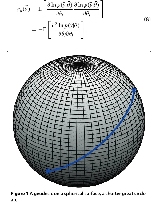
Whenψ(t)is (locally) the shortest paths between two points,ψ(t)is called ageodesicof( ,g): this is the exten-sion of the notion of a straight line to non-Euclidean spaces.
A clear example of a geodesic in a non-Euclidean space is the shortest path on the spherical surface. There are no straight lines here: the shortest path between two points on the spherical surface is the shorter great circle arc (see Figure 1).
In IG, the metric tensor is defined by the Fisher infor-mation matrix. The Fisher inforinfor-mation matrix is defined for some likelihood functionp(y|θ)and parameter vector
θas the expectation value
gij(θ) =E
∂lnp(y|θ) ∂θi
∂lnp(y|θ) ∂θj
= −E
∂2lnp(y|θ)
∂θi∂θj
.
(8)
In this paper, we will study the basic case for range only. For this one-dimensional case, the Fisher information metric reduces to
Distances on this one-dimensional statistical manifold can simply be calculated fromds2 = G(τ)dτ2(e.g., [5]). We will derive an expression for the Fisher information metricG(τ)for arbitrary waveforms in the next part.
2.3.1 Information distance cell design
We derive the Fisher information metricG(τ)to design and construct grid cells with a constant information dis-tance as they support radar resolution. In the derivation ofG(τ), we closely follow the approach from [6]. How we construct the grid cells differs from the previous works (e.g., [5] and [6]) as we directly incorporate the delay-dependent amplitude and use raw radar measurements in the data model. This is incorporated by letting the signal amplitudeabe a function of delay, i.e.,a → a(τ). The signal amplitudea(that is independent ofτ) is our refer-ence case. The received signal is modeled in continuous form as
y(t)=a(τ)s(t−τ)+z(t), (10)
wheres(t−τ)is a replica of the transmitted signal delayed by τ andz(t)is the zero-mean, complex Gaussian noise with varianceγ. The measurementyis complex Gaussian, defined by
p(y|τ)⇔CN(a(τ)s(t−τ),γ ). (11)
The probability density functionp(y|τ)is given by
p(y|τ)= 1
whereτ is the parameter of interest. The Fisher informa-tion metric is given by Equainforma-tion 9, or
G(τ)= −
∞
−∞
∂2lnp(y|τ)
∂τ2 p(y|τ)dy. (13) In order to avoid certain convergence problems [17], we divide the likelihood function to obtain a likelihood ratio (y|τ), which is again a likelihood function:
(y|τ)= pp(y)(y|τ). (14)
is independent ofτ, we know that
E
so we can continue to find the Fisher information metric based on(y|τ). We then take the natural logarithm of
Differentiating twice with respect toτresults in
∂2(y|τ)
Taking the expectation value and multiplying by −1 gives the Fisher information metric
G(τ)= γ2
∞
−∞
∂a(τ)∂τs(t−τ)2dt. (19) Note that for the reference case, this result reduces to
G0= In previous work, the resultG0was derived and the sub-stitution a → a(τ) was made to incorporate the delay into the Fisher information. The difference from current work is that the delay dependence in the Fisher infor-mation metric G(τ) was derived by incorporating the fundamental radar equation in the model of raw data.
2.4 Delay-dependent amplitude and phase-modulated waveforms
From the fundamental radar equation (e.g., [18]), we know that the received power scales withτ−4. This means that the amplitude of the received signal can be written as
a(τ)= b
τ2, (21)
withb some complex parameter that may include gain, RCS, etc. The delay-dependent Fisher information metric G(τ)from Equation 19 can then be written as
In order to apply the previous equation to a test case, we define the unit energy replica of the transmitted waveform with square envelope and phase modulation (PM)ϕ(t)as
s(t)= 1
Tp
exp [iϕ(t)] fort∈[ 0,Tp] , (23)
whereTpis the pulse duration andϕ(t)is a real, differen-tiable function on the interval [ 0,Tp] that represents the phase of the signal. Note that using this construction, the frequency and phase modulation is controlled byϕ(t)and the amplitude bya(τ). The first derivative is calculated as
∂s(t−τ)
where the constantC is specific for a waveform and its PM, defined as
Information distances on both manifolds are calcu-lated intrinsically different. For the reference case, it is a Euclidean metric, i.e.,
d0(τa,τb)=
G0(τa−τb), (28)
while the distance on the new manifold, with delay-dependent amplitude control is calculated as
d(τa,τb)=
With these results, the grid cells will be constructed in the next part.
2.4.1 Choice of the cell size
Using the expression in Equation 29, we have to con-struct resolution cells. For this, we need to determine the information distance of one grid cellδ. We start with the calculation of the total information distance of the listen-ing interval, i.e. the time interval betweenTp and pulse repetition time (PRT),d(Tp, PRT) and the choice of an
appropriate number of grid cellsNcells. Combining these, the size of the information grid cell is determined through
δ= d(Tp, PRT)
Ncells
. (30)
Note that in the current analysis, the relative size of the grid cell with respect to the total PRT δ/d(Tp, PRT) is independent of parametersbandγ because they are held constant.
An alternative method is to (experimentally) determine at what distance the conventional resolution (from the ref-erence grid) is ‘correct’. The conventional resolution cell at this positionm(and thus given on the interval [τm,τm+1]) determines the size of the information resolution cell
δ=d(τm,τm+1). (31) Another possibility is to use the method from [5]. This paper uses information distance in a Monte Carlo method for determining whether there are one or two targets present in a small area. The critical distance for the model radar in distinguishing the two targets with some empiri-cal probability of error is defined as the resolution cell.
When the value forδis determined, the new resolution grid is constructed by starting atτ1 = Tp and iterating along the PRT
τi+1=argτ[d(τi,τ)−δ=0] . (32) Note that when Equation 30 is used, this results in an integer number of grid cells on the listening interval.
Processing on the grid will be done with SSP. For this, the coherence of the sensing matrix c(A) must be low. This is not the case when the grid cells are too close together, which leads to a lower bound in grid cell size. This coherence-adjusted grid is designed for the practical case in Section 3.
2.4.2 LFM pulse
We apply the above results to the test case of a linear chirp (LFM pulse) of bandwidthB. The phase is given by
ϕ(t)=πB
Now, constant Cfor this waveform is calculated from Equation 27 as
C= (πB)
2
12 . (34)
This gives expressions for both metrics,
20 40 60 80 100 120
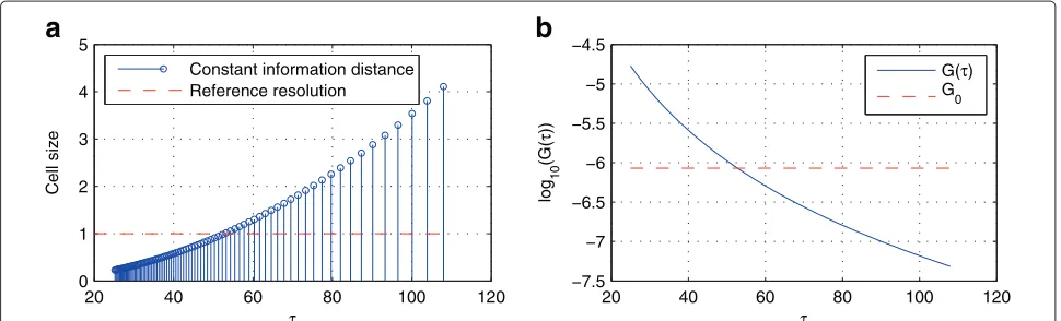
Figure 2Fisher information metrics and grid cell sze.(a)The Fisher information metrics of the amplitude-dependent (constant information distance) model and the reference case.(b)Grid cell size as a function of distance for both models.
The Fisher information metricsG0andG(τ)are shown in Figure 2a.
Distances on the statistical manifold of the delay-dependent case are calculated as
d(τa,τb)=|
By combining the last result with Equations 30 and 32, the cells were constructed and their size is shown in Figure 2b.
3 Numerical results
The information-based design and processing with the adaptive grid will be demonstrated using simulated data in the basic case of range only in pulse radar. We consider the LFM pulse from Equation 33 and set parameterbto be|b| = 1, the pulse lengthTp = 25, the bandwidthB equal to the normalized sampling frequencyfs,B=fs=1, PRT=108, and varianceγ =1. Note that no compressive acquisition is involved yet but regular Nyquist sampling in the observation grid (as we focus here on the estimation grid).
We first determine the total information distance dur-ing the listendur-ing time on the PRT:d(Tp, PRT). Then, we determine a desirable number of cellsNcells: for this par-ticular case, we setNcells = PRT−Tp = 83, which is the same number of cells as for the reference case. From this, in Equations 30 and 32, we calculate the constant information distanceδand construct the grid cells, which are found in Figure 3. Note that our analysis holds for all the radar types providingG(τ)from Equation 26 with the waveform specific constantCin and the parameterbthat includes the gain, RCS, etc. The sensing matricesAand
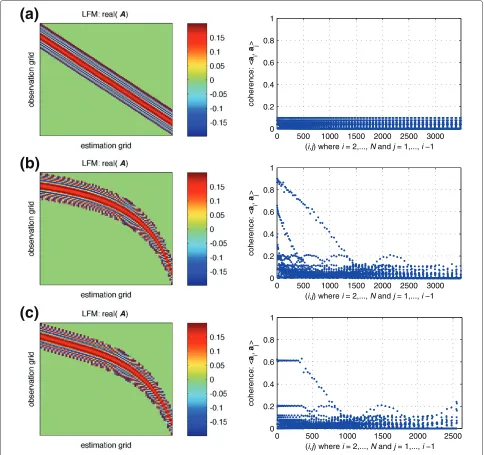
corresponding coherencesc(A)are illustrated in Figure 4. SSP on the grids is shown in Figure 5.
The reference grid (Figure 3) causes the coherence to be low and its maximum is constant for all ranges (Figure 4a). The information-based grid (Figure 3) leads to higher coherence for close ranges because of the smaller cells (Figure 4b). An optimal smallest grid size is to be designed as a compromise between the information-based distance (Equation 29), the incoherence of the sensing matrix (Equation 3), operational needs, and the available processing power.
The coherence of the sensing matrixc(A)is taken into consideration after the grid cells are determined with the constant information distanceδ. For very small grid cells, the coherence is very high. An attempt in lowering the coherence is made by setting the minimum cell size to half the cell size of the reference case. For the test case, this means that for all cells withτ <37 the cell size is fixed, as is seen in Figure 3 and Figure 4c.
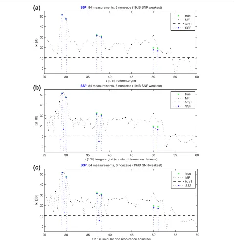
In a range-only case, we show an example of the radar operation where closer ranges may have a higher priority. In our test case, there are three pairs of targets at differ-ent ranges from radar, where each pair consists of two targets that are equally distant from each other at every of
25 30 35 40 45 50 55 60
Figure 4Sensing matrices and corresponding coherences.Sensing matrix (left) and coherence plot (right) for the reference grid(a), the constant information distance grid(b), and the coherence-adjusted grid(c). Note that in (c), the sensing matrix contains less elements because a lower bound on cell size has been applied in order to limit the coherence, hence the lower number of column combinations(i,j).
the three different ranges (Figure 5). The distance between the two targets in a pair is equal to one unit cell from the reference grid. On the reference grid (Figure 5a), the targets cannot be resolved at any range. SSP on both irreg-ular grids (Figure 5b,c) enables resolving the two targets at closer ranges but on the coherence-adjusted grid with less cells. The coherence-adjusted grid (Figure 5c) is an exam-ple how the grid can be adapted by limiting its cell size to the half as it is small enough for a given scenario, and moreover, it lowers coherence (Equation 3) as well as the
computational demands. We applied anad hoc cell size that illustrates the design compromise well.
4 Conclusions
25 30 35 40 45 50 55 60 0
10 20 30 40 50
τ [1/B]: irregular grid (coherence adjusted)
|
x
| [dB]
SSP: 84 measurements, 6 nonzeros (19dB SNR weakest)
true MF
h:γ 1
SSP
25 30 35 40 45 50 55 60
0 10 20 30 40 50
τ [1/B]: irregular grid (constant information distance)
|
x
| [dB]
SSP: 84 measurements, 6 nonzeros (19dB SNR weakest)
true MF
h:γ 1
SSP
25 30 35 40 45 50 55 60
0 10 20 30 40 50
τ [1/B]: reference grid
|
x
| [dB]
SSP: 84 measurements, 6 nonzeros (19dB SNR weakest)
true MF
h:γ 1
SSP
(a)
(b)
(c)
Figure 5Results of SSP on the reference grid (a), information-based grid (b), and coherence-adjusted grid (c).The closer targets are only resolved on the irregular grids. The coherence-adjusted grid gives the best results.
In addition, we also explore how such an irregular esti-mation grid suits radar processing in practice, propose applying SSP from CS, and adjust the grid accordingly for this type of processing.
The IG-based grid and its processing by SSP enable the adaptive grid adjustments that ensure better radar per-formance and more efficient radar processing because the processing power and resolution are optimized over ranges. Thus, such an adaptive grid compromises the
IG-based grid with the CS-IG-based sensing incoherence and naturally, also with the available processing power and operational demands. In existing radar processing, there is no flexibility in the FFT-based grid.
Competing interests
The authors declare that they have no competing interests.
Author details
1Department of Applied Physics, University of Groningen, Groningen 9747 AG, The Netherlands.2Sensors Advanced Developments Delft, Thales Nederland B.V., Delft 2628 XH, The Netherlands.
Received: 19 February 2014 Accepted: 15 May 2014 Published: 30 May 2014
References
1. AJ den Dekker, A van den Bos, Resolution: a survey. J. Opt. Soc. Am. A.
14(3) (1997)
2. CE Cook, M Bernfeld,Radar Signals; An Introduction to Theory and Application. (Academic Press, 1967)
3. E de Jong, R Pribi´c,Design of radar grid cells with constant information distance. (SEE Radar, Lille, France, 2014)
4. E de Jong, R Pribi´c, Sparse-signal processing on information-based range grid, inIEEE Workshop SAM, A Coruña, Spain, (2014)
5. Y Cheng, X Wang, T Caelli, X Li, B Moran, On information resolution of radar systems. IEEE Trans. Aero. Electron. Syst.48(4), 3084–3102 (2012). http://dx.doi.org/10.1109/TAES.2012.6324679
6. P Stinco, Performance analysis of bistatic radar and optimization methodology in multistatic radar system. PhD thesis, University of Pisa (2012)
7. R Pribi´c, I Kyriakides, Design of sparse-signal processing in radar systems, inIEEE Conference ICASSP(Florence, Italy, 2014)
8. D Donoho, Compressed sensing. IEEE Trans. Inform. Theor.52(4), 1289–1306 (2005)
9. M Herman, T Strohmer, High-resolution radar via compressive sensing. IEEE Trans. Signal Process.57(6), 2275–2284 (2009)
10. S Kay, The geometry of statistical inference, inPlenary at IEEE Workshop SAM, (2012)
11. JA Trop, SJ Wright, Computational methods for sparse solution of linear inverse problems. Proc. IEEE.98(6), 948–958 (2010)
12. L Zegov, R Pribi´c, G Leus, Optimal waveforms for compressive sensing radar, inEUSIPCO(Marrakech, Morocco, 2013)
13. R Pribi´c, HJ Flisijn,Back to Bayes-ics in Radar: Advantages for Sparse-Signal Recovery. (CoSeRa, Bonn, 2012)
14. PM Woodward,Probability and Information Theory, with Applications to Radar, (Pergamon, 1953)
15. SD Babacan, R Molina, AK Katsaggelos, Bayesian compressive sensing using laplace priors. IEEE Trans. Image Process.19(1), 53–63 (2010). http://dx.doi.org/10.1109/TIP.2009.2032894
16. B O’Neill,Elementary Differential Geometry, Revised 2nd Edition. (Elsevier, 2006)
17. HL Van Trees,Detection, Estimation and Modulation Theory, Part I. (Wiley-VCH Verlag GmbH & Co. KGaA, 2001), pp. 238–356 18. N Levanon,Radar Principles. (Wiley-VCH, 1988)
doi:10.1186/1687-6180-2014-78
Cite this article as:de Jong and Pribi´c:Sparse signal processing on estimation grid with constant information distance applied in radar.
EURASIP Journal on Advances in Signal Processing20142014:78.
Submit your manuscript to a
journal and benefi t from:
7Convenient online submission
7Rigorous peer review
7Immediate publication on acceptance
7Open access: articles freely available online
7High visibility within the fi eld
7Retaining the copyright to your article