A Reduced-Complexity Fast Algorithm for Software
Implementation of the IFFT/FFT in DMT Systems
Tsun-Shan Chan
VXIS Technology Corporation, Hsin-chu, Taiwan, ROC Email: [email protected]
Jen-Chih Kuo
Department of Electrical Engineering, Graduate Institute of Electronics Engineering, National Taiwan University, Taipei 106, Taiwan, ROC
Email: [email protected] An-Yeu (Andy) Wu
Department of Electrical Engineering, Graduate Institute of Electronics Engineering, National Taiwan University, Taipei 106, Taiwan, ROC
Email: [email protected]
Received 31 August 2001 and in revised form 15 May 2002
The discrete multitone (DMT) modulation/demodulation scheme is the standard transmission technique in the application of
asymmetric digital subscriber lines (ADSL)andvery-high-speed digital subscriber lines (VDSL). Although the DMT can achieve higher data rate compared with other modulation/demodulation schemes, its computational complexity is too high for cost-efficient implementations. For example, it requires 512-point IFFT/FFT as the modulation/demodulation kernel in the ADSL systems and even higher in the VDSL systems. The large block size results in heavy computational load in running programmable digital signal processors (DSPs). In this paper, we derive computationally efficient fast algorithm for the IFFT/FFT. The proposed algorithm can avoid complex-domain operations that are inevitable in conventional IFFT/FFT computation. The resulting soft-ware function requires less computational complexity. We show that it acquires only 17% number of multiplications to compute the IFFT and FFT compared with the Cooly-Tukey algorithm. Hence, the proposed fast algorithm is very suitable for firmware development in reducing the MIPS count in programmable DSPs.
Keywords and phrases:FFT, IFFT, DMT, software implementation.
1. INTRODUCTION
Recent progress of Internet access has a strong demand on high-speed data transmission. To overcome the transmission bottleneck over the conventional twisted-pair telephone lines, several sophisticated modulation/demodulation schemes have been proposed, including carrierless-amplitude-phase (CAP) modulation [1], discrete multitone modulation (DMT) [2, 3, 4, 5] and QAM technology [6]. Among these advanced modulation schemes, the DMT can achieve highest transmission rate since it incorporates lots of advanced DSP techniques such as dynamic bit allocation, multidimensional tone encoding, frequency-domain equal-ization, and so forth. As a consequence, the DMT has been chosen as the physical layer transmission standard by the ADSL standardization committee.
One major disadvantage of the DMT scheme is its high
Modulator
X(0)
X(1)
X(2)
X(0)
X(1)
X(2) Encoded
complex symbols (from encoder)
X(N−1)
X(N)
2
N
-point
IFFT
Pa
ra
ll
el
/S
er
ia
l
Con
ju
ga
te
X(2N−2)
X(2N−1)
y(n)
Channel y˜(n)
Demodulator ˜
X(0) ˜
X(1) ˜
X(2) ˜
X(0) ˜
X(1) ˜
X(2)
Ser
ial/P
ar
allel
2
N
-point
FFT
˜
X(N−1)
˜
X(2N−2) ˜
X(2N−1)
Discar
d
Demodulated complex symbols (to decoder) .
. .
. . .
. . .
. . . . . .
Figure1: The IFFT/FFT block diagram in the DMT system.
The new scheme can avoid redundant complex-domain of the IFFT/FFT. That is, it involves only real-valued opera-tions to compute the IFFT/FFT. Hence, we can avoid the spe-cial data structure in software programming to run complex-domain addition/multiplication operations in computing the IFFT/FFT. In addition, our analysis shows that we need only 17% and multiplications in computing the IFFT and FFT compared with Cooly-Tukey algorithm [10]. The low computational complexity as well as real-domain operations makes it very suitable for firmware coding in DSPs, which helps to save the MIPS counts. Also, the DSP program can be written in recursive form which requires less ROM/RAM program storage space to implement the IFFT/FFT.
The rest of this paper is organized as follows. Section 2 shows the derivation of the IFFT algorithm. In Section 3, the derivation of the FFT algorithm is discussed. The computa-tion complexity comparison is shown in Seccomputa-tion 4. The finite precision effect of our algorithm is also discussed. Finally, we conclude our work in Section 5.
2. REDUCED-COMPLEXITY IFFT ALGORITHM
2.1. The IFFT derivation
The IFFT/FFT block diagram in the DMT system is showed in Figure 1. At the transmitter side, to ensure the IFFT gen-erates only real-valued outputs, the inputs of the IFFT in the DMT standard have the constraint [11],
X(0)=X(N)=0,
X(k)=X∗(2N−k) fork=1,2, . . . , N−1, (1)
whereX(k)=Xr(k) + j·Xi(k) are encoded complex sym-bols. As defined in [12, Chapter 9], the IFFT of a finite-length sequence of length 2Nis
x(n)= 1 2N·
2N−1
k=0
X(k)W2−nkN
, forn=0,1, . . . ,2N−1,
(2) where
Wnk 2N=exp
−j2πnk 2N
=cos2πnk
2N −jsin 2πnk
2N . (3)
By decomposingninto the first half and the second half, (2) becomes
x(n)= 1
2N · N−1
k=0
X(k)W2−nkN + 2N−1
k=N
X(k)W2−nkN
. (4)
Next, by substituting (3) into (4), and using (1), we can sim-plify (4) as (see Appendix A)
x(n)=N1 ·
N−1
k=0
Xr(k) cos22πnkN − N−1
k=0
Xi(k) sin22πnkN
= 1
N·
MDCT(n)−MDST(n),
forn=0,1, . . . ,2N−1.
Xr(0)
Xr(1)
. . .
Xr(N−2)
Xr(N−1)
Even-odd index mapping
Xr(0)
Xr(2) . . .
Xr(N−4)
Xr(N−2)
Xr(1)
Xr(3) . . .
Xr(N−5)
Xr(N−3)
Xr(N−1) + . . . + +
N/ 2-point MDCT
g(n)
N/ 2-point MDCT
h(n)
xr(N−1)
−xr(N−1) + + . . .
xr(N−1) −xr(N−1)
+ +
Γ0
Γ1 . . . ΓN/2−2
ΓN/2−1 . . .
+ +
. . . + +
+
+ + . . . + +
+ +
−
−
−
MDCT (0) MDCT (1)
. . .
MDCT (N/2−2) MDCT (N/2−1)
Special case
MDCT (N/2) MDCT (N/2 + 1) MDCT (N/2 + 2)
. . . MDCT (N−1)
Odd summation
Injected items
Γn=1/2Cn2N
n: 0∼N/2−1
N-point MDCT
Xr(k) 1-point MDCT
MDCT (n) Xr(k) MDCT (n)
Figure2:N-point MDCT(n) butterfly structure, where 1-point MDCT is the minimum-sized processing block.
From (5), we can see that the computation of the IFFT is decomposed into two real-valued operations. One is a discrete cosine transform DCT-like operation with Xr(k), k = 0,1,2, . . . , N −1, as the inputs. The other is a dis-crete sine transform DST-like operation with Xi(k), k =
0,1,2, . . . , N − 1, as the inputs. We will name the first term Modified DCT (MDCT), and the second term Modi-fied DST (MDST). Note that the MDCT and MDST involve only real-valued operators. Furthermore, it can be shown that
MDCT(n)=MDCT(2N−n), forn=0,1, . . . , N−1, (6)
MDST(n)= −MDST(2N−n), forn=0,1, . . . , N−1. (7)
Hence, we can focus on computing MDCT(n) and MDST(n) forn=0,1, . . . , N−1. Then, expand the results forn=N+ 1, N+ 2, . . . ,2N−1. For the special cases ofn=0 andn=N, the MDCT and MDST can be simplified as
MDCT(0)=
N−1
k=0
Xr(k) cos2π0k 2N =
N−1
k=0 Xr(k),
MDST(0)=
N−1
k=0
Xi(k) sin2π0k 2N =0,
MDCT(N)=
N−1
k=0
Xr(k) cos2πNk 2N =
N−1
k=0
Xr(k)(−1)k,
MDST(N)= N−1
k=0
Xi(k) sin2πNk 2N =0,
(8)
respectively. These simple relationships can help us to save additional computation complexity.
2.2. MDCT/MDST operations of the IFFT
of the MDCT. We follow the derivation in [9] and define Cnk
2N =cos(2πnk/2N). Then, the MDCT can be written as
MDCT(n)=
N−1
k=0
Xr(k)Cnk2N, forn=0,1, . . . , N−1. (9)
Decompose the MDCT into even and odd indices ofk, then (9) can be rewritten as
MDCT(n)=g(n) +h(n), forn=0,1, . . . ,N
2 −1, (10)
where
g(n)=
N/2−1
k=0
Xr(2k)C2nN(2k)= N/2−1
k=0
Xr(2k)CNnk,
h(n)=N/2−1 k=0
Xr(2k+ 1)Cn2N(2k+1).
(11)
Defineh(n)=2C2nNh(n). Following the derivation in Lee’s algorithm [9], we can find
MDCT(n)=g(n) +h(n)=g(n) + 1
2C2nNh(n). (12)
That is,
N−1
k=0
Xr(k)C2nkN N-point MDCT
=
N/2−1
k=0
Xr(2k)CnkN N/2-point MDCT, g(n)
+ 1 2Cn2N
N/2−1
k=0
Xr(2k+ 1) +Xr(2k−1)CnkN
N/2-point MDCT, h(n)
+Xr (N−1)(−1)n
injected item ,
forn=0,1, . . . ,N 2 −1.
(13)
On the other hand, by replacing indexnwith (N−n) in (12), it can be shown that
MDCT(N−n)=g(n)−h(n)=g(n)− 1
2C2nNh(n). (14)
The special case MDCT(N/2) needs to be computed sepa-rately, which can be simplified as
MDCT N
2
=
N−1
k=0
Xr(k)C2kN(N/2)=
N−1
k=0
Xr(k) coskπ 2 . (15)
The mapping of (13), (14), and (15) is shown in Figure 2. As we can see, theN-point MDCT is decomposed into twoN/
2-point MDCT (g(n) andh(n)) plus some pre-processing and post-processing modules. Then we can apply the technique of divide-and-conquer to recursively expand the N/2-point MDCT until 1-point MDCT is formed. That is, we repeat the decomposition in (10) and (11) untilN=1.
Next, we consider the recursive implementation of the MDST. We defineSnk2N = sin (2πnk/2N). As with the deriva-tion in (10), (11), (12), (13), and (14), we can find
MDST(n)=
N/2−1
k=0
Xi(2k)SnkN
+ 1 2Cn2N
N/2−1
k=0
Xi(2k+ 1) +Xi(2k−1)SnkN,
MDST(N−n)= −
N/2−1
k=0
Xi(2k)SnkN
+ 1 2Cn2N
N/2−1
k=0
Xi(2k+ 1) +Xi(2k−1)SnkN,
forn=0,1, . . . ,N 2 −1.
(16)
It is worth noting that the injected item is zero in the MDST. Besides, the MDST also has a special case for indexN/2 as
MDST N
2
=
N−1
k=0
Xi(k)Sk2N(N/2)= N−1
k=0
Xi(k) sinkπ2 . (17)
The mapping of the MDST structure in Figure 3 is similar to the MDCT structure, except that minimum processing block is 2-point MDST (see Figure 3) and the injected items do not exist in the MDST implementation. That is, we repeat the de-composition in (16) untilN=2. Note that the 1-point MDST is always equal to zero.
2.3. Overall IFFT computation procedures
The overall IFFT computation flow is shown in Figure 4. It consists of the MDCT/MDST operations and a post-processing operation. The operations in Figure 4 are as fol-lows:
(1) set the butterfly operation to MDCT mode;
(2) Xr(k),k = 0,1, . . . , N −1, are first fed into the but-terfly architecture to obtain the MDCT(n), for n =
0,1, . . . , N−1;
(3) the post-processing operation expands the N-point MDCT outputs to 2N-point MDCT using the sym-metric property in (6);
(4) set the butterfly operation to MDST mode;
(5) repeat the computation in Steps 2 and 3 usingXi(k), k=0,1, . . . , N−1 as inputs, and obtain the MDST(n), forn=0,1, . . . , N−1;
Xi(0)
N-point MDST
Xi(k0)
Figure3:N-point MDST(n) butterfly structure, where 2-point MDST is the minimum-sized processing block.
(7) based on (5), we combine the MDCT and MDST re-sults together with the scaling operation (which is achieved by shifting right by log2(N) bits) to obtain the IFFT results. This is done in the post-processing operation.
2.4. Matrix notation of the MDCT/MDST
In this section, we present the matrix notation of the pro-posed fast IFFT algorithm. The matrix form can help to see the divide-and-conquer nature of our approach. By follow-ing the notation in [13], we rewriteXr(k) and MDCT(n) as
respectively. Then (9) can be represented as
MDCT(n)N=TN,MDCT
Xr(k)N, (20)
where [TN,MDCT] denotes the transform kernel matrix of the
MDCT operation. Next, the injected items of (13) can be
represented as
We define theodd-summation matrixas
and thescaling matrixas
The special case of the MDCT in (15) can be represented as
MDCT N
2
Xi(0)
Figure4: The proposed IFFT architecture.
where
[JN/2] denotes the opposite-diagonal identity matrix. We can
also represent (20) and (27) in the recursive form as shown in Figure 5. Following the above derivations, the matrix no-tation of transform kernel of the MDST can be derived as
MDST is similar to the MDCT except that there is no in-jected items. Also, the special case matrix can be modified as
SN=0 1 0 −1 0 · · · −1. (29)
The block diagram of the MDST in the matrix form is shown in Figure 6.
3. REDUCED-COMPLEXITY FFT ALGORITHM
3.1. The FFT derivation
At the receiver side (see Figure 1), the 512-point FFT is used to demodulate the received signals, which is given by
˜ Hence, (30) can be rewritten as
˜
Xr(0)
Xr(1)
. . .
Xr(N−2)
Xr(N−1)
Even-odd index mapping
Even
Odd
[TN/2]
[TN/2] [LN/2]
Xr(N−1) [Q N/2]
[SN]
+ [ΦN/2]
+ +
+
+ +
−
[JN/2] MDCT (n)N
Figure5: Block diagram of the MDCT operation in matrix form.
Xi(0)
Xi(1)
. . .
Xi(N−2)
Xi(N−1)
Even-odd index mapping
Even
Odd
[TN/2]
[TN/2] [LN/2]
[SN]
[ΦN/2]
+ + +
+ +
− [JN/2] MDST (n)N
Figure6: Block diagram of the MDCT operation in matrix form.
decomposed into a combination of two real-domain kernels—MDCT(k) and MDST(k). Both MDCT and MDST use ˜x(n), n = 0,1, . . . ,2N −1, as the inputs. Hence, we only employ two real-valued kernels (MDCT and MDST), thus no complex-valued operations are required in com-puting the FFT. In addition, in the DMT system, the lower N-point FFT outputs are conjugate-symmetric to the up-perN-point outputs. We are only interested inN-point data fork = 0,1, . . . , N −1. Hence, we can neglect the outputs
˜
X(k),fork=N, N+ 1, . . . ,2N−1.
3.2. MDCT/MDST operations of the FFT
In (32), the transform kernels are 2N-point MDCT(k) and MDST(k). Here, we propose a novel approach to further re-duce the computational complexity. Hence, we only need to performN-point MDCT/MDST.
We first decompose input sequence into a symmet-ric sequence, ˜xc(n), plus an antisymmetric sequence, ˜xs(n), where
˜
xc(n)=1
2
˜
x(n) + ˜x(2N−n),
˜ xs(n)=1
2
˜
x(n)−x˜(2N−n), forn=1,2, . . . , N−1. (33)
Hence, we have
˜
x(n)=xc˜(n) + ˜xs(n), (34)
˜
x(2N−n)=x˜c(n)−x˜s(n), forn=1,2, . . . , N−1. (35)
By substituting (34) and (35) into (30), we can simplify (30) as (see Appendix B)
˜ X(k)=
˜
x(0) + ˜x(N)(−1)k
+ 2 N−1
n=0
˜
xc(n) cos2πnk 2N −j
N−1
n=0
˜
xs(n) sin2πnk 2N
=x˜(0) + ˜x(N)(−1)k+ 2MDCT(k)−jMDST(k),
fork=0,1, . . . , N−1,
(36)
where ˜xc(0)=0 and ˜xs(0)=0. Since the block size is reduced from 2N-point (see (32)) toN-point (see (36)).
MDCT(k)=g(k) + 1
Similarly, for the MDST(k), we have
MDST(k)=g(k) + 1
The two special cases for indexN/2 are
MDCT
The block diagram of the MDCT(k) is shown in Figure 7. The mapping of the MDST structure is similar to the MDCT structure in Figure 7 except that minimum processing block is 2-point MDST and the injected items do not exist in the MDST(k) implementation (see Figure 8). Then we can just combine the MDCT(k) and MDST(k) outputs, followed by adding ˜x(0) and ˜x(N)(−1)k, to obtain the FFT results based on (36).
3.3. Overall FFT computation procedures
The overall computation flow of the FFT is shown in Figure 9. The operations are as follows.
(1) The received signals ˜x(n),n = 0,1, . . . ,2N−1, are decomposed to ˜xc(n) and ˜xs(n),n=0,1, . . . , N−1, through the pre-processing operation.
(2) In the first phase, the generated ˜xc(n) are fed into re-cursive butterfly operation to obtain the MDCT(k) outputs. (3) In the second phase, we repeat the computation by using the ˜xs(n) as inputs into recursive butterfly operation to obtain the MDST(k) outputs.
(4) We combine the MDCT(k) and MDST(k) results then add ˜x(0) and ˜x(N)(−1)ktogether to obtain the FFT re-sults based on (36). This is done in the post-processing oper-ation.
3.4. Matrix notation of the MDCT/MDST
Based on (19), (20), (21), (22) (23), (24), (25), and (26), we can represent (37), (38), and (39) as
MDCT(k)/MDST(k), respectively. The block diagrams of the MDCT(k) and MDST(k) are very similar to the MDCT(n) and MDST(n) in Section 2. The difference is that it requires a pre-processing to compute the ˜xc(n) and ˜xs(n). The block diagrams of the MDCT and MDST are shown in Figures 10 and 11, respectively.
4. COMPLEXITY COMPARISON AND FINITE-PRECISION EFFECT
4.1. Comparison of hardware complexity
˜
N-point MDCT
˜
xc(n) 1-point MDCT
MDCT(k) x˜c(n) MDCT(k)
Figure7:N-point MDCT(k) butterfly structure, where 1-point MDCT is the minimum-sized processing block of the FFT module.
2N-point
N-point MDST ˜
2N-point ˜
x(0) ˜
x(1)
. . .
˜
x(2N−2) ˜
x(2N−1) Pre-processing
N-point N-point ˜
xs(0),x˜c(0) ˜
xs(1),x˜c(1)
. . .
. . .
˜
xs(N−2),x˜c(N−2) ˜
xs(N−1),x˜c(N−1) 2nd
phase 1st phase
N-point MDCT(1st phase) MDST(2nd phase)
˜
x(0) + ˜x(N)(−1)k
+ R X˜(0)
. . .
. . . ˜
x(0) + ˜x(N)(−1)k
+ R X˜(N/2)
. . .
. . . ˜
x(0) + ˜x(N)(−1)k
+ R X˜(N−1)
Post-processing
Figure9: The proposed FFT architecture.
˜
x(0) ˜
x(1)
. . .
˜
x(2N−2) ˜
x(2N−1) Pre-processing
˜
xs(0) ˜
xs(1)
. . .
˜
xs(2N−2) ˜
xs(2N−1)
Even-odd index mapping
Even
Odd [LN/2]
˜
xc(N−1)
[TN/2]
[TN/2]
[ON/2]
[SN]
+ [ΦN/2]
+ +
+
+ −
+ [JN/2] MDCT (k)N
Figure10: Block diagram of the MDCT in matrix form for the FFT operation.
˜
x(0) ˜
x(1)
. . .
˜
x(2N−2) ˜
x(2N−1) Pre-processing
˜
xs(0) ˜
xs(1)
. . .
˜
xs(N−2) ˜
xs(N−1)
Even-odd index mapping
Even
Odd [L N/2]
[TN/2]
[TN/2]
[SN]
[ΦN/2]
+ +
+
+ −
+ [JN/2] MDST (k)N
Figure11: Block diagram of the MDST in matrix form for the FFT operation.
algorithm. The corresponding butterfly architecture requires log2(2N) stages in the 2N-point IFFT/FFT. Each stage consists of N multiplications and 2N additions. Because
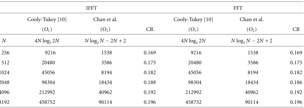
Table1: Comparison of computational complexity for 2N-point IFFT/FFT.
IFFT FFT
Cooly-Tukey [10] Chan et al. Cooly-Tukey [10] Chan et al.
(O1) (O2) CR (O1) (O2) CR
N 4Nlog22N Nlog2N−2N+ 2 4Nlog22N Nlog2N−2N+ 2
256 9216 1538 0.169 9216 1538 0.169
512 20480 3586 0.175 20480 3586 0.175
1024 45056 8194 0.182 45056 8194 0.182
2048 98304 18434 0.188 98304 18434 0.186
4096 212992 40962 0.192 212992 40962 0.192
8192 458752 90114 0.196 458752 90114 0.196
(a) Number of multiplication operations.
IFFT FFT
Cooly-Tukey [10] Chan et al. Cooly-Tukey [10] Chan et al.
(O1) (O2) CR (O1) (O2) CR
N 6Nlog22N (9/2)Nlog2N+N+ 1 6Nlog22N (9/2)Nlog2N+N
256 13824 9473 0.685 13824 9472 0.685
512 30720 21249 0.692 30720 21248 0.692
1024 67584 47105 0.697 67584 47104 0.697
2048 147456 103425 0.701 147456 103424 0.701
4096 319488 225281 0.705 319488 225281 0.705
8192 688128 487425 0.708 688128 487424 0.708
(b) Number of addition operations.
multiplication. Also, it takes 2 real additions to realize a com-plex addition. As a result, the direct approach requires a to-tal of 4Nlog2(2N) real multiplications and 6Nlog2(2N) real additions. The large computation complexity are not suitable for cost-effective realization of the IFFT/FFT modules in the DMT system.
The complexity comparison for 2N-point IFFT/FFT are listed in Table 1. Thecomplexity ratio (CR)is defined as
CR= O2 O1,
(44)
whereO1andO2are the number of multiplications (or
ad-ditions) in other fast algorithms and our approach, respec-tively. We can see that the complexity ratio of the multi-plication is only 17% for N =256 compared with conven-tional IFFT/FFT. Table 1 also shows that our approach can gain more computation savings asNgets larger in the VDSL systems [14].
4.2. Experiment results
There are lots of DSP processors on the market. Due to the variety or hardware structure, coding styles, compli-ers, and so forth, we are not trying to do the detail op-timization for specific processors. On the other hand, we would like to compare the proposed algorithm with Cooly-Tukey’s algorithm, which is a baseline of the FFT realiza-tion. The implementation platform is TI TMS320C54 eval-uation board, http://www.ti.com. Both algorithms are writ-ten in C language without any assembly-level program-ming tricks. During compilation, the TI C54X C com-plier is used without adding special compilation options, neither.
Table2: Comparison of clock cycle for Cooley-Tukey FFT and pro-posed recursive algorithm.
128-point 256-point 512-point
Cooley-Tukey FFT 16,485 37,118 82,347
Proposed 11,869 25,726 55,435
Clock cycle Ratio 28% 31% 33%
0 5 10 15 20 25 30 35 40 45 50
Wordlength (B) 0
50 100 150 200
A
ver
aged
SNR
(dB)
Direct butterfly approach Our approach
(a)
0 5 10 15 20 25 30 35 40 45 50
Wordlength (B) 0
50 100 150 200
A
ver
aged
SNR
(dB)
Direct butterfly approach Our approach
(b)
Figure12: Averaged SNR versus wordlength for the 512-point (2N
value) (a) IFFT. (b) FFT.
4.3. Finite-precision effect
In fixed-point implementation of the IFFT/FFT kernels, it is important to consider the effects of finite register length in the IFFT/FFT calculations (see [12, Chapter 9] and [15]). To compare the butterfly approach and our approach in fixed-point implementation, we conduct extensive computer sim-ulation by using MATLAB for finite-wordlength IFFT/FFT architecture. Figure 12 shows the SNR performance with as-signed wordlength B =8, 16, 32 bits. We observe that the SNR performance withB=16 bits is good enough in prac-tical fixed-point implementations. From the simulation re-sults, we can see that the SNR performance of our approach is comparable to the traditional butterfly approach under the same wordlength.
5. CONCLUSIONS
In this paper, we develop a computationally efficient fast al-gorithm for the software implementation of the IFFT/FFT kernel in the DMT system. We reformulate the IFFT/FFT functions so as to avoid complex-domain operations. The complexity ratio of the multiplications is only 17% compared with the direct butterfly implementation approach. The pro-posed algorithm provides a good solution in reducing MIPS count in programmable DSP implementation for the appli-cations of the DMT transceiver systems.
APPENDICES
A. DERIVATION OF (4)
Decomposing (4) into the first half and second half with the fact thatX(0)=X(N)=0, (4) can be represented as
x(n)= 1
2N · N−1
k=1
X(k)W2−nkN + 2N−1
k=N+1
X(k)W2−nkN
. (A.1)
Usek=2N−kto replace the variable in the second term. Then, we have
x(n)= 1 2N·
N−1
k=1
X(k)W2−nkN + 1
k=N−1
X(2N−k)W2−N(2N−k)n
.
(A.2) Becausekis a dummy variable, we can rewrite (A.2) as
x(n)= 1
2N · N−1
k=1
X(k)W2−nkN + N−1
k=1
X(2N−k)W2−N(2N−k)n
= 1
2N · N−1
k=1
X(k)W2−nkN + N−1
k=1
X(2N−k)W2−N2NnW2nkN
.
(A.3)
By using the facts that
W2Nn 2N =1,
Wnk 2N =exp
−j2πnk 2N
=cos2πnk
2N −jsin 2πnk
2N ,
W−nk 2N =exp
j2πnk
2N
=cos2πnk
2N +jsin 2πnk
2N ,
X(0)=X(N)=0,
(A.4)
we can rearrange (A.3) to
x(n)= 1
N · N−1
k=0
Xr(k) cos2πnk
2N −Xi(k) sin 2πnk
2N
.
B. DERIVATION OF (30)
Equation (30) can be represented as
˜
X(k)=x˜(0)+ ˜x(N)(−1)k+ N−1
n=1
˜
x(n)W2nkN+
2N−1
n=N+1
˜ x(n)W2nkN
.
(B.1) Usen =2N−nto replace the variable in the second term. Then, we have
˜
X(k)=x˜(0) + ˜x(N)(−1)k
+ N−1
n=1
˜
x(n)W2nkN+
1
n=N−1
˜
x(2N−n)Wk(2N−n) 2N
.
(B.2)
Becausenis a dummy variable, we can rewrite (B.2) as
˜
X(k)=x˜(0) + ˜x(N)(−1)k
+ N−1
n=1
˜
x(n)W2nkN+ N−1
n=1
˜
x(2N−n)W2kN(2N−n)
=x˜(0) + ˜x(N)(−1)k
+ N−1
n=1
˜
x(n)W2nkN+ N−1
n=1
˜
x(2N−n)W22NkNW2−nkN
.
(B.3)
By using the fact thatW22NkN=1 and applying the assumption of the input data in (35), we can rearrange (B.3) as
˜
X(k)=x˜(0) + ˜x(N)(−1)k
+ 2 N−1
n=1
˜
xc(n) cos2πnk 2N −j
N−1
n=1
˜
xs(n) sin2πnk 2N
.
(B.4)
ACKNOWLEDGMENT
T. S. Chan is with the VXIS Tech. Corp. Hsin-Chu, Taiwan, ROC. This work is supported in part by the National Science Council, ROC, under Grant NSC 87-2213-E-008-011.
REFERENCES
[1] G. H. Im, D. D. Harman, G. Huang, A. V. Mandzik, M. H. Nguyen, and J. J. Werner, “51.84 Mb/s 16-CAP ATM LAN standard,”IEEE Journal on Selected Areas in Communications, vol. 13, no. 4, pp. 620–632, 1995.
[2] J. S. Chow, J. C. Tu, and J. M. Cioffi, “A discrete multitone transceiver system for HDSL applications,” IEEE Journal on Selected Areas in Communications, vol. 9, no. 6, pp. 895–908, 1991.
[3] K. Sistanizadeh, P. Chow, and J. M. Cioffi, “Multi-tone trans-mission for asymmetric digital subscriber lines (ADSL),” in
Proc. IEEE International Conf. on Communications, vol. 2, pp. 756–760, Geneva, Switzerland, 1993.
[4] I. Lee, J. S. Chou, and J. M. Cioffi, “Performance eval-uation of a fast computation algorithm for the DMT in high-speed subscriber loop,” IEEE Journal on Selected Areas in Communications, vol. 13, no. 9, pp. 1560–1570, 1995.
[5] T. N. Zogakis, J. T. Aslanis Jr., and J. M. Cioffi, “A coded and shaped discrete multitone system,” IEEE Trans. Communica-tions, vol. 43, no. 12, pp. 2941–2949, 1995.
[6] B. Daneshrad and H. Samueli, “A 1.6 Mbps digital-QAM sys-tem for DSL transmission,” IEEE Journal on Selected Areas in Communications, vol. 13, no. 9, pp. 1600–1610, 1995. [7] B. R. Wiese and J. S. Chow, “Programmable implementations
of xDSL transceiver systems,” IEEE Communications Maga-zine, vol. 38, no. 5, pp. 114–119, 2000.
[8] A.-Y. Wu and T. S. Chan, “Cost-efficient parallel lattice VLSI architecture for the IFFT/FFT in DMT transceiver technol-ogy,” inProc. IEEE Int. Conf. Acoustics, Speech, Signal Pro-cessing, pp. 3517–3520, Seattle, Wash, USA, May 1998. [9] B. G. Lee, “A new algorithm to compute the discrete cosine
transform,”IEEE Trans. Acoustics, Speech, and Signal Process-ing, vol. 32, no. 6, pp. 1243–1245, 1984.
[10] J. W. Cooly and J. W. Tukey, “An algorithm for the machine calculation of the complex Fourier series,” Math. Comp., vol. 19, pp. 297–301, April 1965.
[11] ANSI Standard T1.413, “Network and customer installation interface-Asymmetric digital subscriber line (ADSL) metallic interface,” 1995.
[12] A. V. Oppenheim and R. W. Schafer,Discrete-Time Signal Pro-cessing, Prentice-Hall, Englewood Cliffs, NJ, USA, 1989.
[13] H. D. Yun and S. U. Lee, “On the fixed-point-error analysis of several fast DCT algorithms,”IEEE Trans. Circuits and Systems for Video Technology, vol. 3, no. 1, pp. 27–41, 1993.
[14] T1E1.4/2000-013R3, “Very-high-speed digital subscriber lines (VDSL) metallic interface, part 3: Technical specification of a multi-carrier modulation transceiver,” 2000.
[15] K. J. R. Liu, A.-Y. Wu, A. Raghupathy, and J. Chen, “Algorithm-based low-power and high-performance multi-media signal processing,”Proceedings of the IEEE, vol. 86, no. 6, pp. 1155–1202, 1998, Special Issue on Multimedia Signal Processing.
Tsun-Shan Chanwas born in Chang-Hui, Taiwan, ROC, in 1973. He received his M.S. degree in electrical engineering from the National Central University, Taiwan, in 1998. During 1998–1999, he worked on communication applications in Industrial Technology Research Institute, Hsin-Chu, Taiwan. Since 1999, he has been serving as a system engineer of the video processing projects in VXIS Technology Corporation.
An-Yeu (Andy) Wu received his B.S. de-gree from National Taiwan University in 1987, and the M.S. and Ph.D. degrees from the University of Maryland, College Park in 1992 and 1995, respectively, all in elec-trical engineering. During 1987–1989, he served as a signal officer in the Army, Taipei, Taiwan, for his mandatory military service. During 1990–1995, he was a graduate teach-ing and research assistant with the