Differences in ground motion and fault rupture process between the surface and
buried rupture earthquakes
Takao Kagawa1, Kojiro Irikura2, and Paul G. Somerville3
1Geo-Research Institute, 4-3-2 Itachibori, Nishi-ku, Osaka 550-0012, Japan 2Disaster Prevention Research Institute, Kyoto University, Japan
3URS Corporation, USA
(Received July 22, 2003; Revised December 19, 2003; Accepted December 26, 2003)
We have studied differences in ground motion and fault rupture characteristics between surface rupture and buried rupture earthquakes. We found that the ground motion generated by buried rupture in the period range around 1 second is on average 1.5 times larger than the average empirical relationship. In contrast, ground motion from earthquakes that rupture the surface is 1.5 times smaller in the same period range. This phenomenon is considered to be caused by differences in fault rupture process between the two types of earthquakes. To examine possible reasons of the above effect we analyzed source slip distribution data derived from waveform inversions, and divided them into two groups: surface rupture and buried rupture earthquakes. It was found that the large slip areas (asperities) of surface rupture earthquakes are concentrated in the depth range shallower than about 5 km. In contrast, large slip areas of buried rupture earthquakes are spread over the depth deeper than 5 km. We also found that the total rupture area of buried rupture earthquakes is 1.5 times smaller than that of surface rupture earthquakes having the same seismic moment, and that deep asperities have about 3 times larger effective stress drops and 2 times higher slip velocities than shallow asperities. These observations are verified by numerical simulations using stochastic Green’s function method.
Key words:Strong ground motion, surface rupture fault, buried rupture fault, rupture process, asperity, stress drop, slip velocity.
1.
Introduction
Empirical attenuation relationships are commonly used to predict earthquake strong ground motions. In the attenua-tion relaattenua-tionships, the seismic engineering parameters (such as peak acceleration or response spectrum) are related to the source/site parameters (e.g. source magnitude, hypocen-tral distance and site soil conditions) on an empirical basis. Although such attenuation relations are based on recorded strong motion data, the limited number of model parameters and the simplified functional form of the attenuation relation-ships does not allow it to achieve high prediction accuracy. Recent seismological development have lead to new predic-tion techniques, that are based on wave propagapredic-tion calcula-tions using detailed velocity structure including the site, and on the asperity model of the seismic source.
To employ the asperity source model for the prediction of strong ground motions, the characterized asperity model was introduced (e.g. Somervilleet al., 1999; Miyakoshiet al., 2000). In this model, the complex slip distribution of a real earthquake is represented by a few rectangular as-perities with uniform slip distribution embedded in a fault plane having lower background slip. Based on the analysis of many source slip inversion results of crustal earthquakes, Somervilleet al.(1999) introduced scaling relationships for
Copy right cThe Society of Geomagnetism and Earth, Planetary and Space Sciences (SGEPSS); The Seismological Society of Japan; The Volcanological Society of Japan; The Geodetic Society of Japan; The Japanese Society for Planetary Sciences; TERRA-PUB.
parameters of the characterized asperity model. Irikuraet al. (2001) proposed a recipe for the prediction of strong ground motions from future earthquakes that is based on the charac-terized asperity model and on the scaling relations adapted to Japan. The main scaling parameter is the seismic moment M0.
In this work we introduce more detailed aspects of the earthquake source by considering differences in source char-acteristics and ground motion charchar-acteristics between sur-face rupture and buried rupture crustal earthquakes. Here we define a surface rupture earthquake as an earthquake which has clear surface dislocation caused by the earthquake, and significant slip at shallow depth (shallower than 5 km), as inferred from slip model inversion. On the other hand, we define a buried rupture earthquake as an earthquake that does not have clear surface dislocation and shallow slip. Prelim-inary analysis of Somerville (2003) shows that the ground motions of the buried ruptures are stronger than the ground motions of surface ruptures in the period range aroundT =1 sec. The importance of this observation is enhanced by the fact that some buried rupture earthquakes occur on buried faults which have no surface trace and whose locations are unknown in some cases.
We first compare the observed ground motions for surface ruptures and buried ruptures, following to Somerville (2003). Then, we analyze the depth distribution of the asperities of the available slip models, and re-estimate the asperity locations based on the original slip distribution data and on
Fig. 1. Ratio of response spectra of recorded ground motions to that of an empirical attenuation relationship for the cases of surface rupture earthquake (top and center) and buried rupture earthquake (bottom). The zero line represents the level of the empirical attenuation relationship. Lines above the zero line indicate an event’s ground motion exceeding the model.
the results of analysis of the distribution of asperities with depth. Finally, separate scaling relationships are derived for surface ruptures and buried ruptures. These results are verified by numerical simulations using the stochastic Green function method.
2.
Observed Difference in Ground Motions
be-tween Buried and Surface Rupture Earthquakes
Table 1. Numbers of rock and soil sites of the records used in the Fig. 1. Italic fonts indicate earthquakes that are not used in the empirical relationship by Abrahamson and Silva (1997).
(bottom). The plots indicate residuals between the ground motions of selected individual earthquakes and the empiri-cal ground motion attenuation relationship of Abrahamson and Silva (1997), i.e. event term, versus period. The zero line represents the model of Abrahamson and Silva (1997) that takes into account the magnitude, distance, and site con-ditions. Lines above the zero line indicate an event whose ground motion exceeds the model level. Here, 0.4 natural log units equals a factor of nearly 1.5. Some of the earth-quakes treated in the Fig. 1 occurred after 1997, so the event terms were not calculated by Abrahamson and Silva (1997). For these earthquakes, we use the residuals between the data and the model to represent the event term.
In the period range around 1 second (sayT =0.5–3.0 sec), the ground motions from magnitude MW = 6.5–7.0 earth-quakes without surface rupture (bottom panel) are clearly larger than the average level (∼1.5 times). In the period rangeT =0.3–3.0 sec, the ground motions from the earth-quakes with similar magnitude, that produced large tectonic surface rupture, are significantly weaker (∼1.5 times) even though rupture occurred at the surface (center). We catego-rize the 1995 Kobe earthquake as a buried rupture earthquake because the strong ground motions observed in the Kobe City area are affected by the north-east portion of the fault which does not have surface break. Similar trends are present for the 1999 Kocaeli, Turkey and 1999 ChiChi, Taiwan earth-quakes (top), which have larger magnitudeMW >7.0. Be-cause the ground motions are averaged over many records at various site conditions for each earthquake, the event terms pertain to the effects of the earthquake source. Table 1 shows the numbers of rock and soil sites of the records used in the Fig. 1. From the table, it appears that the Kocaeli, Kobe and Imperial Valley event terms might be biased by site condition effects, but the event terms for the other earthquakes are not likely to be biased.
We conclude that the ground motion generated by buried rupture earthquakes is larger than the ground motion gen-erated by surface rupture earthquakes. This phenomenon
is considered to be caused by differences in the fault rup-ture process between these two types of earthquakes. In this paper we study differences in rupture parameters, namely: rupture area, asperity area, asperity depth, stress drop of the fault, stress drop of the asperities, and slip velocity.
3.
Depth Distribution of Asperities
Somerville et al. (1999) analyzed the slip distributions of 15 crustal earthquakes derived by waveform inversion mainly from strong ground motion data. The slip models that we used were developed using a fairly uniform pro-cedure, mostly by the technique proposed by Hartzell and Heaton (1983). The resolution of shallow slip is important for this study. Strong ground motions are sensitive to shal-low slip, because shalshal-low slip causes large surface waves. For this reason, we expect that the resolution of shallow slip should be quite good. For example, Wald and Heaton (1994) analyzed the 1992 Landers earthquake using geodetic data, strong ground motion data, teleseismic data, and combined data. The slip model obtained using strong ground motion data alone yielded a distribution of surface slip that is similar to that obtained by the other data sets, and to the observed slip distribution.
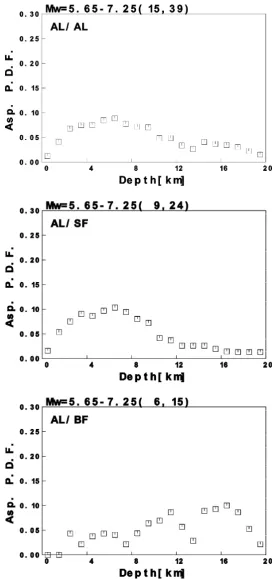
Fig. 2. Depth distribution of the probability density function of asperity location according to the data of Somervilleet al.(1999). The top, center, and bottom panels show the cases of all earthquakes, surface rupture earthquakes, and buried rupture earthquakes respectively.
separately in this work, based on the original field data. Figure 2 clearly demonstrates that asperities of surface rupture earthquakes are concentrated in the shallow depth range between 2 and 10 km, and asperities of buried rupture earthquakes are distributed almost uniformly with depth in the upper crust at depths greater than 5 km.
4.
Identification of Shallow and Deep Asperities
in-Table 2. Fault parameters of the analyzed earthquakes.
Fig. 3. An example of the asperity identification procedure. The top panel shows the slip distribution in the 1992 Landers Earthquake (Wald and Heaton, 1994). The center and bottom panels show asperities identified without and with partition into shallow and deep asperities respectively.
clude the 1984 Nagano (Yoshida and Koketsu, 1990), 1997 Kagoshima, 1997 Yamaguchi and 1998 Iwate (Miyakoshi et al., 2000) and 2000 Tottori (Sekiguchi and Iwata, 2001) earthquakes in Japan, the 1999 Kocaeli earthquake in Turkey (Sekiguchi and Iwata, 2002) and 1999 ChiChi earthquake, Taiwan (Iwata et al., 2000). Except for the 1984 Nagano earthquake, the slip models were derived using the same
Fig. 4. Categorization of the considered earthquakes into four groups. The horizontal line separates earthquakes with and without shallow asperities, and vertical line separates earthquakes with and without surface breaks.
(1994). An elongated zone of large shallow slip is present just beneath the surface break. The center panel of the fig-ure shows the result of characterizing slip model using the methodology of Somerville et al.(1999). This process in-corporated part of the shallow large slip zone into a deep asperity. We used an automated computer-based procedure to identify asperities, following the criteria of Somervilleet al.(1999), p. 64.
Next, we identified shallow asperities and deep asperi-ties. We first identified asperities from the slip distribution shallower than 5 km and then we identified deeper asperities from the remaining portion of the fault. We defined the crit-ical depthhc = 5 km as the best value using a grid search in the depth rangeh =3–8 km, by analyzing the fault rup-ture models of all earthquakes. The bottom panel of Fig. 3 shows the asperities identified in this manner. The effective stress drops are also indicated in the figure. They were esti-mated assuming a circular crack model (Eshelby, 1957) for the deep asperities (Eq. (1)) where M0 andS indicate seis-mic moment and area of an asperity. A semi-ellipsoid crack model (Watanabeet al., 1998) was applied for the shallow open asperity (Eq. (2)) where the aspect ratio (length (L) over width (W)) is assumed to be two and Poisson’s ratio (ν) is assumed to be 0.25.
Shallow asperities have smaller effective stress than deeper asperities.
Applying the above analysis to all earthquakes, we ob-tained two groups of earthquakes: those with shallow as-perities and those without shallow asas-perities. Then, by
di-viding the earthquakes into events with surface rupture and without surface rupture following Wells and Coppersmith (1994), we divided all the treated earthquakes into the four groups shown in Fig. 4. In this figure, the upper portion con-tains earthquakes with shallow asperities and the lower half shows those without shallow asperities. Also, the right por-tion indicates earthquakes with surface breaks and the left portion indicates earthquakes without surface breaks. The events in the upper right quadrant are defined as pure surface rupture earthquakes and those in the lower left quadrant are defined as pure buried rupture earthquakes. Here the 1995 Kobe earthquake is categorized as a surface rupture earth-quake because it has clear surface break and shallow asper-ity, although they did not affect the strong ground motion observed in the Kobe City area as mentioned before. We used the data of these two groups for further analysis.
5.
Scaling Relationships of Surface and Buried
Rupture Earthquakes
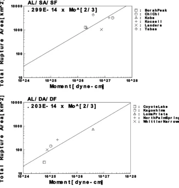
Here we analyzed scaling characteristics of both types of earthquakes. First, we analyzed the macroscopic fault rupture parameters, i.e. the total rupture area A0, the stress dropσ0and the ratio of the combined asperity area to the fault area Aa/A0. Figure 5 and Table 3 show the result-ing scalresult-ing relationships between these parameters and the seismic momentM0. Here we used the scale invariant, self-similarity assumption, i.e. A0 ∼ M02/3, σ0 = const and
Aa/A0=const.
Fig. 5. Scaling relationship between fault rupture area and seismic moment. The self-similar least squares fit lines for surface rupture (upper panel) and for buried rupture (lower panel) are indicated.
Table 3. Scaling relations for the whole ruptures: rupture areaA0versusM0, stress dropσ0, and the ratio of the combined asperity area to the fault area
Aa/A0.
ratio is almost same as the standard error of each scaling relationship, indicating the difference is significant despite the small number of analyzed earthquakes. The average effectiveσ value for buried rupture earthquakes is almost 2 times larger than that for earthquakes with surface rupture. Standard deviations from the averages are shown in the table. The standard deviations are not small enough, however, the difference of the average values between the two types of earthquake is significant enough. The ratios of the asperity
area to the fault area Aa/A0 are practically the same for these two cases. Standard deviations of the values are also indicated in the table.
(a)
(b)
(c)
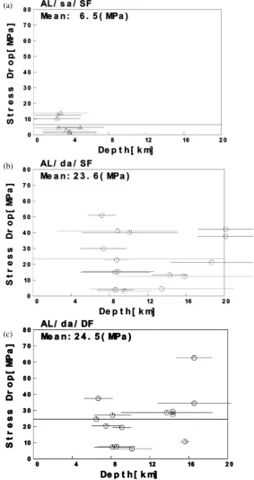
Fig. 6. Depth distribution of effective stress drops estimated for asperities. Asperities (from top to bottom) are indicated by horizontal lines, and circle marks are the centroids of each asperity. (a) Shallow asperities of surface rupture earthquakes. (b) Deep asperities of surface rupture earthquakes. (c) Deep asperities of buried rupture earthquakes.
Figure 6 and Table 4 show the depth distribution ofσa. From the figure, we can clearly see that theσavalues of the shallow asperities are much smaller (∼3 times) than those of the deep asperities. Deep asperities both on surface rupture faults and on buried rupture faults have almost the same stress drop,σa = 23.6±15.2 MPa and σa = 24.5± 14.5 MPa respectively. Standard deviations are evaluated similarly as Table 3. The values of the effective stress drops of shallow and deep asperities seem to have large scatter
when the values from all of the earthquakes are combined. However, the ratio of stress drops between shallow and deep asperities of each earthquake has less scatter, and is a factor of about three. The scatter in the effective stress drops of asperities is considered to be caused by the distribution of average stress drops of the individual earthquakes shown in Table 3.
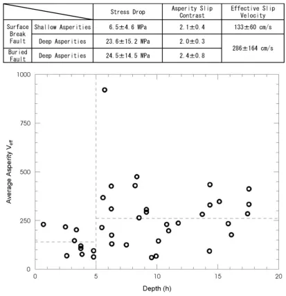
Table 4. Scaling parameters (theconstvalues) for individual asperities: effective stress dropsσa, asperity slip contrastDa/D0and slip velocityVe f f.
Fig. 7. Depth distribution of slip velocity for all asperities. Indicated depths are the centroids of the asperities.
deep asperities are about twice those of the shallow asperi-ties: 133±60 cm/s and 286±164 cm/s respectively. The outlier in Fig. 7, from the 1985 Oct. Nahanni earthquake, makes the standard deviation large. Values of the asperity slip contrast Da/D0 in Table 4 are practically the same for the shallow and deep asperities.
We consider the significant differences of effective stress drop and slip velocity between shallow and deep asperities reflect the depth dependency of these values in the crustal layer. However, the depth dependency is not gradual but abrupt at a depth around 5 km. This critical depth might have local and regional variations.
6.
Simulation of Strong Ground Motions of
Shal-low and Buried Earthquakes
To test whether the derived differences in the source char-acteristics can explain the observed differences in the ground motions between the two types of earthquakes, we con-structed examples of the characterized fault rupture models
for surface and buried rupture earthquakes, and calculated the strong ground motion records in the near fault region by the stochastic Green’s function method (Boore, 1983; Kamae and Irikura, 1992).
(a)
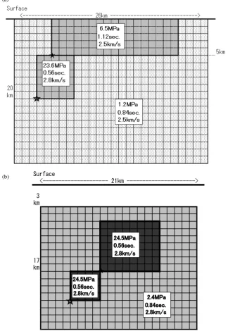
(b)
Fig. 8. Standard characteristic slip models for (a) surface rupture fault and (b) buried rupture fault;MW =6.5 in both cases. The largest shallow asperity on surface rupture fault was set between 0 and 5 km depth; it has lower effective stress drop, longer rise time and slower rupture velocity than the deep asperity.
Table 5. Velocity and attenuation structures assumed for strong ground motion simulation.Qvalues are explained as functions of frequencyf.
were set at 80% of the shear wave velocityVS. Locations of the rupture starting points, asperities, and sites were almost the same for the surface and for the buried rupture earth-quakes.
To avoid generation of surface fault rupture, following
Fig. 9. Results of the dynamic simulation of generation of tensile cracks due to variation of top depth of asperity (Dalguer and Irikura, 2002, courtesy of Luis Angel Dalguer). Distributions of newly generated tensile cracks (diagonal thin lines) around the main fault (vertical thick line) are shown in the panels. When the top depth of the asperity becomes 5 km, tensile cracks barely reach the surface.
Fig. 10. Site locations for strong ground motion simulation.
Fig. 11. Comparison of the simulated response spectra with the empirical spectral attenuation relationship of Abrahamson and Silva (1997). Compare this figure with Fig. 1.
parameter shown in Fig. 8. They found that if the asperity depth equals or exceeds 5 km, the probability that the crack reaches the surface is very low.
We calculated ground motion response spectra for 21 sites on a 5 ×5 km grid shown in Fig. 10. Figure 11
the ground motions between the surface and buried rupture earthquakes in Fig. 11 have similar characteristics to those of the observed ground motions shown in Fig. 1. In the pe-riod range around 1 second, the ground motion due to buried rupture earthquake is larger than that from surface rupture earthquake, even though the surface rupture earthquake has a shallow asperity close to the surface and to the near-fault sites. Thus, we can conclude that the combined effect due to the differences in the (1) rupture area versus magnitude scaling, (2) depth of asperities, (3) their effective stress drop and slip velocity, is able to produce the observed difference in ground motions between the two types of earthquakes.
7.
Discussion and Conclusions
Differences were identified in the ground motion and in the fault rupture characteristics between surface and buried rupture earthquakes. It was found and confirmed by the nu-merical simulations that in the period range around 1 sec, the ground motions from buried rupture earthquakes are signif-icantly larger than the ground motions from surface rupture earthquakes.
At first glance this observation contradict the observation of large damage of buildings in surface rupture earthquakes such as the 1999 ChiChi, Taiwan, and 1999 Kocaeli, Turkey, earthquakes, in spite of them having lower ground motions than average (see Fig. 1, top panel). However, more detailed analysis in case of the 1999 ChiChi, Taiwan earthquake, shows that the damage was concentrated in a very narrow belt-like zone along fault, where the surface dislocation due to fault rupture could directly affect the buildings. This kind of phenomenon is usually reported through field surveys of earthquake damage, e.g. the 1990 Philippine earthquake, the 1995 Kobe, Japan, earthquake, and the 1999 Kocaeli, Turkey, earthquake. This suggests that the buildings were damaged mainly by the effects of surface dislocation, not by the strong ground motion.
The result derived here is important for evaluating the near-field ground motion for both surface rupture and buried rupture earthquakes. It is desirable to perform additional numerical verification of these observations using dynamic source simulations with realistic parameters.
The main results of the study are as follows.
1) Ground motion generated by buried rupture earthquakes in the period range around 1 second is larger than the ground motion generated by surface rupture events.
2) The large slips of surface rupture earthquakes are con-centrated in the shallow portion of the fault.
3) The total rupture area of buried rupture earthquakes is smaller than that of surface rupture earthquakes. The effective stress drop of buried rupture earthquakes is larger than that of surface rupture earthquakes.
4) Deep asperities have larger effective stress drops and higher slip velocities than shallow asperities.
5) Ground motions simulated using fault rupture models constructed according to the above results demonstrate
spectral differences between surface and buried rupture earthquakes similar to observed differences.
Acknowledgments. We would like to thank Ken Miyakoshi, To-motaka Iwata, Haruko Sekiguchi, and David J. Wald for their works on waveform inversion. Without their efforts, we could not com-plete this study. Anatoly Petukhin kindly proofread the manuscript and made technical corrections. We also thank associate editor and reviewers for suggestions that improved this paper.
References
Abrahamson, N. A. and W. J. Silva, Empirical response spectral attenuation relations for shallow crustal earthquake,Seism. Res. Lett.,68, 94–127, 1997.
Boore, D., Stochastic simulation of high-frequency ground motions based on seismological models of the radiation spectra,Bull. Seism. Soc. Am., 73, 1865–1894, 1983.
Dalguer, L. A. and K. Irikura, Generation of tensile cracks during a 3D dynamic shear rupture propagation, Japan Earth and Planetary Science Joint Meeting, S042-P017 (CD-ROM), 2002.
Dalguer, L. A., K. Irikura, and J. D. Riera, Simulation of tensile crack generation by three-dimensional dynamic shear rupture prop-agation during an earthquake, J. Geophys. Res., 108(B3), 2144, doi:10.1029/2001JB001738, 2003.
Eshelby, J. D., The determination of the elastic field of and ellipsoidal inclusion, and related problems,Proc. Roy. Soc.,A241, 376–396, 1957. Hartzell, S. H. and T. H. Heaton, Inversion of strong ground motion and
tele-seismic waveform data for the fault rupture history of the 1979 Imperial Valley, California, earthquake,Bull. Seism. Soc. Am.,73, 1,553–1,583, 1983.
Irikura, K., H. Miyake, T. Iwata, K. Kamae, T. Kagawa, and K. Miyakoshi, A recipe of strong motion prediction for scenario earthquake, AGU Fall Meeting, S31C-01, 2001.
Iwata, T., H. Sekiguchi, and A. Pitarka, Source and site effects on strong ground motions in near-source area during the 1999 Chi-Chi, Taiwan, earthquake, AGU Fall Meeting, S72-P05, 2000.
Kamae, K. and K. Irikura, Prediction of site-specific strong ground motion using semi-empirical methods, 10WCEE, 801–806, 1992.
Miyakoshi, K., T. Kagawa, H. Sekiguchi, T. Iwata, and K. Irikura, Source characterization of inland earthquakes in Japan using source inversion results, 12WCEE, 1850, CD-ROM, 2000.
Sekiguchi, H. and T. Iwata, Source process inversion and near-source ground motion simulation of the 2000 Tottoriken-Seibu, Japan, earth-quake (MW6.8), AGU fall meeting, S42C-0654, 2001.
Sekiguchi, H. and T. Iwata, Rupture process of the 1999 Kocaeli, Turkey earthquake estimated from strong-motion waveforms,Bull. Seism. Soc. Am.,92, 300–311, 2002.
Shimazaki, K., Small and large earthquake: the effects of thickness of seismogenic layer and the free surface, inEarthquake Source Mechan-ics,AGU Monograph, 37 (Maurice Ewing Ser. 6), edited by S. Das, J. Boaghtwright, and C. H. Sholz, pp. 209–216, 1986.
Somerville, P. G., Magnitude scaling of the near fault rupture directivity pulse,Phys. Earth Planet. Int.,137, 201–212, 2003.
Somerville, P. G., K. Irikura, R. Graves, S. Sawada, D. Wald, N. Abraham-son, Y. Iwasaki, T. Kagawa, N. Smith, and A. Kowada, Characterizing earthquake slip models for the prediction of strong ground motion,Seism. Res. Lett.,70, 59–80, 1999.
Wald, D. J. and T. H. Heaton, Spatial and temporal distribution of slip of the 1992 Landers, California earthquake,Bull. Seism. Soc. Am.,84, 668–691, 1994.
Watanabe, M., T. Sato, and K. Dan, Scaling relations of fault parameters for inland earthquakes, 10th Jpn. Earthq. Eng. Symp., 583–588, 1998. Wells, D. L. and K. J. Coppersmith, New empirical relationships among
magnitude, rupture length, rupture width, rupture area, and surface dis-placement,Bull. Seism. Soc. Am.,84, 974–1002, 1994.
Yoshida, S. and K. Koketsu, Simultaneous inversion of waveform and geodetic data for the rupture process of the 1984 Naganoken-Seibu, Japan, earthquake,Geophys. J. Int.,103, 355–362, 1990.