F U L L P A P E R
Open Access
A statistical study of satellite traces and evolution
of equatorial spread F
Viswanathan Lakshmi Narayanan
1,2*, Sukanta Sau
3, Subramanian Gurubaran
4, Kazuo Shiokawa
1, Nanan Balan
1,
Kaliappan Emperumal
3and Samireddipalle Sripathi
4Abstract
The ionosonde observations made at 5-min intervals at the Indian dip equatorial station Tirunelveli (8.7°N, 77.8°E geographic; 1.1°N dip latitude) from March 2008 to February 2009 during the extended solar minimum period are used to study the interlink between equatorial spread F (ESF) and satellite traces (STs) which are assumed to represent tilts in the bottomside iso-electron density surfaces probably caused by large-scale wave-like structures (LSWS). The data show different patterns of ESF onset in the bottomside F region, which are illustrated through examples. In addition, the statistics of occurrence of ST and its relation to the formation of ESF are studied. The results indicate that (1) the zonally drifting ESF irregularities can be differentiated from those forming over the observing station. (2) Nearly half of the ESF events were preceded by ST. (3) In about 30% of the cases of occurrence of ST, ESF was not formed afterwards implying that LSWS may not always lead to ESF. (4) The percentage of ESF following ST was high in summer and increased with the time of the night. (5) Following the first occurrence of ST, the ESF onset was delayed by about 30 min on the average suggesting that ST may be used as a precursor of ESF. (6) Pre-reversal enhancement (PRE) of upward plasma drift was found insignificant during the period of study. The trapping of high-frequency radio waves between the E and F regions during intense sporadic E is also illustrated.
Keywords:Ionosonde; Equatorial spread F; Plasma bubbles; Satellite traces; Large-scale wave-like structures
Background
The spreading of the F region trace in nighttime iono-grams at low latitudes was first noticed in 1930s (Booker and Wells 1938). Since then, different aspects of the phenomenon known as equatorial spread F (ESF) have been studied using ionosondes, VHF radars, airglow
ob-servations, VHF and GPS scintillations, in situ rocket
and satellite measurements, GPS-TEC map, etc. (e.g., Woodman and LaHoz 1976; Rastogi 1977; Weber et al. 1978; Basu and Basu 1981; Prakash et al. 1991; Aggson et al. 1996; Valladares et al. 2004; Park et al. 2013). Those experimental observations and theoretical investi-gations (e.g., Ossakow and Chaturvedi 1978; Zalesak et al. 1982; Kelley and Maruyama 1992; Sekar et al. 1994; Huba et al. 2009) together seem to establish that the
Rayleigh-Taylor instability (RTI) is the causative mechanism behind the formation of ESF.
Under favorable conditions in the evening/nighttime ionosphere, bottomside density perturbations lead to the growth of magnetic field-aligned plasma-depleted re-gions through the RTI mechanism. The plasma-depleted regions known as plasma bubbles often extend well into the topside ionosphere (Woodman and LaHoz 1976). The plasma bubbles host different scale sizes of electron density irregularities that reflect radio waves in a ran-dom manner hindering trans-ionospheric communica-tions. The phenomena have therefore been studied widely with a view to reach a prediction capability. The seasonal dependence of ESF and plasma bubble occur-rence is reasonably well understood based on the align-ment of solar terminator with the magnetic meridian and trans-equatorial meridional winds (Abdu et al. 1981; Maruyama and Matuura 1984; Tsunoda 1985), though their day-to-day variability is not yet understood.
The generation of plasma bubbles requires favorable background ionospheric conditions and a seed perturbation
* Correspondence:[email protected]
1
Solar-Terrestrial Environment Laboratory, Nagoya University, Furo-cho, Chikusa-ku, Nagoya, Aichi, 464-8601, Japan
2
Present address: Indian Institute of Science Education and Research Mohali, Sector 81, Manauli PO 140306, SAS Nagar, India
Full list of author information is available at the end of the article
triggering the instabilities. Earlier studies indicate that fa-vorable background ionospheric condition is brought about by the pre-reversal enhancement (PRE)-induced height rise of the ionosphere (Farley et al. 1970; Abdu et al. 1983; Jayachandran et al. 1993; Fejer et al. 1999). Gravity waves are believed to provide the seed perturbations (Kelley et al. 1981; Balachandran Nair et al. 1992; Abdu et al. 2009; Takahashi et al. 2009; Tsunoda 2010; Narayanan et al. 2012; Patra et al. 2013), though other theories also discuss the generation of the irregularities (e.g., Kudeki and Bhattacharyya 1999). Another important likely source for the seeding discussed in recent years is the large-scale wave-like structures (LSWS) detected by azimuthal scanning VHF radars (Tsunoda 2005, 2008), TEC mea-surements (Thampi et al. 2009), and airglow images (Narayanan et al. 2012). Though the source and nature of LSWS are not understood well, they are recognized as wave-like structures in the bottomside ionosphere with scale sizes of a few hundred kilometers.
The ionograms often reveal the presence of additional traces situated close to the F region trace (1F trace) and its higher order reflections, which are known as satellite traces (STs) (Lyon et al. 1961; Abdu et al. 1981). Tsunoda (2008) suggested that the STs are probably sig-natures of LSWS. In the ionograms obtained at close time intervals, ST often appears before the onset of ESF implying that ST can be regarded as a precursor signa-ture of ESF. In addition, Tsunoda (2012) identified the presence of highly tilted traces in ionograms known as multi-reflected echoes (MRE) and suggested them as probable signatures of larger scale tilts than those that could have led to the formation of ST. More recently, Thampi et al. (2012) and Abdu et al. (2014) studied the relationship between ST and ESF onset.
However, a detailed statistical relationship between ST (or LSWS) and ESF is not yet reported to our know-ledge. We present such a study using the ionosonde ob-servations described in the‘Database’section. Since the ionosonde probes only the bottomside ionosphere, in this article, by ESF we refer to those bottomside irregu-larities associated with ESF which caused the spreading of the F region traces observed in the ionograms. The results are presented and discussed in the ‘Results and
discussions’ section which contains cases of different
types of onset of ESF.
Methods
Database
We use the data from the ionospheric sounding experi-ment made with a Canadian Advanced Digital Iono-sonde (CADI) installed at the Indian dip equatorial station, Tirunelveli (8.7°N, 77.8°E geographic; 1.1°N dip latitude). The observations were made at 5-min intervals from 19 March 2008 to 12 February 2009 during the
extended solar minimum period when magnetic activity was generally quiet (AP <15). However, there were some data gaps during 17 October to 10 November 2008, 9 to 11 December 2008, and 17 to 19 December 2008. The ionosonde comprises a delta-type dipole transmitter an-tenna with a peak power of 600 W. The four center-fed dipole receivers are arranged in a square configuration to receive the reflected echoes from the ionosphere. The ionosonde was swept in the frequency range from 2 to 16 MHz in 295 steps. Though the ionograms were noisy in this site, the F region traces were clear enough for the study. Since this work discusses nighttime phenomena, we note the nights using dates of pre-midnight and post-midnight hours. For example, the night of 1 April 2008 will be noted as 1/2 April 2008. Further, all the data are presented in Indian Standard Time (IST) which is 19 min behind the local solar time at Tirunelveli (for example, 18:00 IST = 17:41 LST).
Results and discussion
Examples of onset of ESF with and without ST
This section presents examples of the different types of ESF onsets observed with and without ST. Figure 1 shows a sequence of ionograms on the night of 6/7 October 2008. The ionogram at 19:20 IST did not show ST or ESF. By 19:30 IST, the F trace was doubled below the critical frequency (or satellite trace appeared just above the 1F trace) and continued until 19:40 IST with-out ESF. Around 19:50 IST, ESF started and became intense with time. It is based on this type of observations that ST (or LSWS) is believed to play a key role in the generation of ESF.
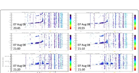
However, on some occasions ST is not observed before the onset of ESF. Figure 2 shows such an example on the night of 7/8 August 2008. As shown, ESF got initi-ated at 21:00 IST without prior ST and developed into intense spreading afterwards. It may be argued that ST could have appeared during the few minutes before the ESF onset at 21:00 IST, the verification of which requires observations at closer than 5-min intervals.
1 1 0 0
2 0 0 4 0 0 6 0 0
Al
t
i
t
u
d
e
(
k
m
)
M H z
Figure 1Example for ESF onset after the occurrence of ST.
1 1 0
0 2 0 0 4 0 0 6 0 0
Al
t
it
u
d
e
(
k
m
)
M H z
patch increases in the later ionograms (compare the iono-grams at 00:20 IST and 00:40 IST). This increase in the virtual height may be due to the increase in the range of the irregularities that are drifting away from the over-head ionosphere horizontally as reported by Calvert and Cohen (1961).
The suggestion is illustrated schematically in Figure 4. Assuming that the irregularities drift horizontally at nearly the same altitude, the range and hence the esti-mated virtual height are higher when the irregularities are in the off-zenith than when they are overhead. The irregularities in Figure 3 therefore appear to drift hori-zontally as reported earlier (Calvert and Cohen 1961; Lynn et al. 2011, 2013; Fagundes et al. 2012). The simple algebraic equations shown in the schematic (Figure 4) can be used to estimate the approximate zonal drift speed. Recently, Lynn et al. (2013) used this technique to estimate the drift speed of the irregularities from the ionograms and showed that they coincide with the movement of plasma bubbles observed in airglow images. The ionograms alone, however, cannot indicate whether
the drift is eastward or westward unless the reception is made with direction-finding capability. However, the drift is generally assumed eastward because plasma bubbles usually drift eastwards (e.g., Chapagain et al. 2013).
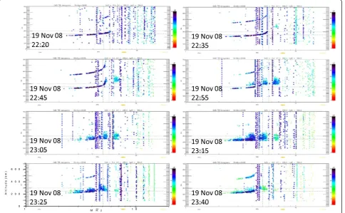
Figure 5 shows an example of the zonal drifting of ESF irregularities on the night of 19/20 November 2008. A small patch of ESF appeared at 22:35 IST around 350-km height range in the ionograms, and the patch oc-curred at the frequencies that are well above the critical frequency of the background ionosphere. The F region trace was unperturbed and clear with a base height at approximately 225 km. In the subsequent ionograms, the ESF patch got intensified, approached the F region trace, and fully covered it by about 23:15 IST. After-wards, the ESF patch was seen to rise slightly in its range until 23:40 IST. The observation can be explained by assuming eastward drifting plasma bubbles (Calvert and Cohen 1961). Initially during 22:35 IST to 23:15 IST, the irregularities entered the ionosonde beam from the west and moved towards the zenith with an estimated drift speed of approximately 110 m/s, and they continued to
1 1 0
0 2 0 0 4 0 0 6 0 0
Al
t
i
t
u
d
e
(
k
m
)
M H z
Figure 3Sudden onset of ESF without the presence of F region trace prior to it.
drift eastward with a speed of approximately 75 m/s. The speeds are within the limit of the drift speeds re-ported earlier (e.g., Chapagain et al. 2013) and they show a reduction in magnitude with time.
When the patch of ESF was first seen at 22:35 IST in Figure 5, it was situated between 6- and 7-MHz frequen-cies while the critical frequency of overhead ionosphere was around 5.5 MHz (see Figure 5). As the ESF patch moved to the overhead sky and continued to approach the 1F trace, its maximum frequency did not decrease but rather stayed nearly stable at approximately 7 MHz. This illustrates that the maximum frequency within the spread F is dependent on the electron densities in the region of irregularities and it does not decrease like the virtual range when the irregularities move towards the overhead sky. In a uniformly stratified ionosphere (within the area covered by ionosonde beam), the electron content can increase in oblique ray paths, but the electron densities will be the same as that for a vertical inci-dence ray path. Since the plasma frequency is propor-tional to the electron density, oblique reflections do not show any pseudo enhancement or reduction in the plasma frequency.
However, since plasma density depletions correspond to ESF irregularities, the frequencies of ESF echoes are not expected to be higher than the critical frequency of
the F region ionosphere. Recently, Abdu et al. (2012) discussed the mechanisms of radio wave echoes due to ESF irregularities and concluded that a significant por-tion arises out of coherent backscattering perpendicular to the magnetic field lines in addition to the total reflec-tions. On the other hand, previous studies indicate that total reflection mechanism explains the observed iono-gram patterns even during ESF times (King 1970; Wright et al. 1996). Further, earlier studies have shown the exist-ence of enhanced electron density regions known as plasma blobs often situated around the electron density depletions (Le et al. 2003; Park et al. 2003; Pimenta et al. 2004). Since ionosonde beam covers a large area, such enhanced electron density regions, if present between adjacent depletions, will also be noticed in the iono-grams. We believe that the ESF reflections at frequen-cies higher than the critical frequency of overhead ionosphere might be due to the presence of plasma blobs in between adjacent plasma depletions hosting the electron density irregularities.
ESF usually starts as range type that turns into fre-quency type (Rastogi 1977; Sastri et al. 1979; Abdu et al. 1981). However, a reverse sequence of development was also observed as illustrated in Figure 6. The spread started near the critical frequency at approximately 23:35 IST on 29/30 April 2008 and subsequently covered
1 1 0
0 2 0 0 4 0 0 6 0 0
Al
t
i
t
u
d
e
(
k
m
)
M H z
the whole 1F trace. It appears that such events also cor-respond to the drifting plasma bubbles. The maximum electron density surrounding the plasma depletions in such cases might be close to that of the peak electron density of the unperturbed background ionosphere. Therefore, such irregularities may be devoid of any plasma blobs around them. In such a case when the ESF irregularities drift from off-zenith locations, the spread will be seen at higher virtual height ranges close to the critical frequency region and will occupy the
whole F region trace when they reach the overhead ionosphere.
Example of ST without ESF
The examples shown above illustrated the development of ESF with or without ST. Recently, Abdu et al. (2014) stud-ied the relationship between the ST and ESF using the digisonde measurements over the dip equator and two magnetically conjugate locations in the Brazilian sector. In their study, STs were observed prior to the onset of ESF
1 1 0
0 2 0 0 4 0 0 6 0 0
A
l
ti
tu
d
e
(
k
m)
M H z
Figure 6Example for ESF onset as frequency type and its expansion to the whole 1F trace.
1 1 0
0 2 0 0 4 0 0 6 0 0
A
l
ti
tu
d
e
(
k
m)
M H z
over the dip equator, and later, STs were detected in the conjugate sites nearly simultaneously prior to the occur-rence of ESF. With such observations during 66 days of solar maximum period, Abdu et al. (2014) suggested that ST might represent early phase of evolution of ESF. How-ever, studies by Narayanan et al. (2012) and Li et al. (2012) have shown cases in which STs were not followed by ESF. The following example illustrates such an observation.
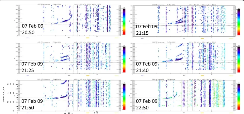
Figure 7 shows an example of ST without the subse-quent generation of ESF at the dip equator on 7/8
February 2009. It can be seen that ST was observed for about 30 min (21:15 IST to 21:40 IST) and no ESF
oc-curred subsequently. As mentioned in the ‘Background’
section, we may consider ST as a manifestation of dy-namically tilted pattern in the bottomside F region which will be the likely seed perturbation for triggering ESF. However, in the case shown in Figure 7, such a seed was present, but plasma irregularities did not develop. That might be because the background conditions were not conducive.
1 1 0
0 2 0 0 4 0 0 6 0 0
A
l t i
t
u
d
e
(
k
m
)
M H z
a
b
c
Other signatures of LSWS
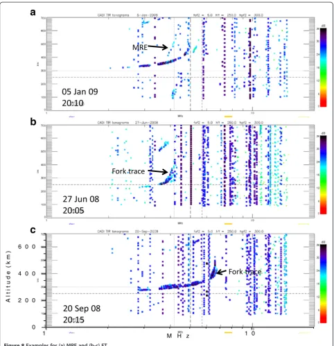
Apart from ST, another ionogram signature conceived to be associated with LSWS is the multi-reflected echoes (or MRE) that appear as highly tilted traces in the iono-grams (Tsunoda 2012; Thampi et al. 2012). Such traces result from the higher order multiple reflections between the ionosphere and ground, which was observed on only one night in our data set as shown in Figure 8a (corre-sponding to the observations of 5/6 January 2009). MREs were rare probably because of the smaller power of the higher order reflections (typically seventh- or eighth-order reflections) which might be below the sen-sitivity level of the instrument. Figure 8b,c shows
exam-ples of what are called ‘fork traces’ (FT) which are
branching of the F trace near the critical frequency. Figure 8b,c was obtained respectively on 27/28 June 2008 and 20/21 September 2008. Such traces were frequently observed by Lyon et al. (1961) along with ST before the formation of ESF. In our data, FT was observed on 30 nights of which 22 nights showed ST as well. In the remaining eight nights, four nights showed the formation of ESF. The purpose of showing MRE and FT (Figure 8) is to indicate that they are probably other signatures of
LSWS. However, since they are infrequent, we discuss the statistics based only on ST.
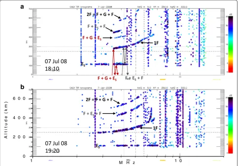
Pseudo ST
Before proceeding to the statistics, we would like to mention about‘pseudo STs’which are not STs but often
observed in the presence of intense sporadic E (ES)
layers. Mixed reflections occur at times when ES layers
are present as described in Piggott and Rawer (1978)
and termed as ‘M reflections’. They arise due to the
combination of multiple reflections between the
iono-spheric F layer, ES layer, and ground. Figure 9 shows
sample ionograms obtained on 7/8 July 2008 illustrating
‘pseudo STs’caused by mixed reflections. The examples indicate that all traces situated between the 1F and 2F traces are not ST. We have taken enough care that such pseudo STs are not counted as STs in the statistical analysis.
Statistics of ST and ESF
STs were often observed in more than one ionogram at 5-min intervals. All ST occurrences within 2 h are con-sidered as one ST event. The ST signatures separated in
1 1 0
0 2 0 0 4 0 0 6 0 0
A
l t i
t u d e
(
k
m )
M H z
a
b
excess of 2 h are considered as separate ST events. Simi-larly, we presume that the ST and ESF are related only if the ESF is observed within 2 h of the last observation of ST. If the time gap was more than 2 h, the ST and ESF are considered to be unrelated. Time gap of up to 2 h seems sufficient for the LSWS to trigger ESF.
In addition to the abovementioned criteria, we con-sider only those STs occurring near the 1F trace and well below the 2F trace. To study the role of LSWS on the generation of ESF, the STs are first identified and those ESFs that follow the STs are identified next. This makes the statistics more robust. Further, we consider only clear STs that are not affected by a spread. Sometimes, STs are observed with a spread (Lynn et al. 2013) which indicates the presence of ESF irregularities at off-zenith locations probably approaching the zenith of the obser-vation site as discussed earlier (refer to Figure 5). The presence of ST without any spread indicates bottomside tilts associated with LSWS, as mentioned above. In this study, we make an attempt to understand the role of such tilts and how often do they lead to the formation of ESF.
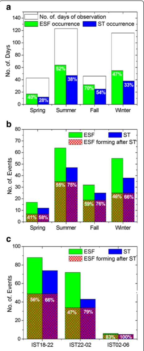
With the above selection criteria, we have observed 122 ST events on the whole of which 86 events (70%) were followed by ESF. A total of 166 ESF events were observed indicating that 52% of the ESF events were formed after the occurrence of ST. Figure 10a shows the seasonal occurrence rate of ESF and ST during the extended solar minimum period considered herein. The periods March to April 2008, May to August 2008, Sep-tember to October 2008, and November 2008 to Febru-ary 2009 are considered as (northern hemisphere) spring equinox, summer, fall equinox, and winter, respectively. The ESF occurrence percentages were maximum during fall equinox and minimum during spring equinox in the extended solar minimum period considered herein. This pattern is different from the usual equinox maxima for the occurrences of ESF in the Indian sector reported earlier (Sastri et al. 1979; Sripathi et al. 2011). The oc-currence pattern of STs was also similar to that of ESF with maximum during fall equinox and minimum dur-ing sprdur-ing equinox. However, the number of ST occur-rence is less than the number of ESF occuroccur-rence revealing that ESF are not always preceded by ST. The absence of ST cannot be taken as an evidence for the absence of LSWS because ST is one of the signatures of LSWS and it is not necessary that the presence of LSWS should always be recorded as ST. Further, since the ionograms are acquired in discrete time steps, ST signa-tures will be missed if they occur between two successive transmissions. Indeed, this is the reason for observing ST more frequently when ionograms are acquired at closely spaced time intervals. The presence of ST thus indicates the existence of LSWS, while its absence does
not preclude LSWS. Therefore, we will focus our discus-sion on the occurrences of ST and the formation of ESF following ST. By this, we attempt to identify how often LSWS signatures lead to the formation of ESF.
Figure 10b shows the seasonal occurrences of ESF and ST along with the number of events in which ESF followed ST. The percentage occurrences of ESF following ST was small during spring equinox (58%) and winter (66%) com-pared to other seasons (76% and 75% during fall equinox and summer, respectively). This pattern is similar to the occurrence rates of ESF and ST separately. Further, the ob-servations are separated into three time bins correspond-ing to 18 to 22 IST, 22 to 02 IST, and 02 to 06 IST as shown in Figure 10c. A significant number of ST occur-rences are observed later in the night indicating that LSWS does not always occur around the post-sunset verti-cal motions associated with PRE. Figure 10c shows that the percentage of ESF following the ST increases with
time. This indicates that LSWS plays comparatively a greater role in triggering ESF later in time when the iono-sphere is less dense. It may be seen from Figure 10c that the number of events was very less during 02 to 06 IST. This observation would have instrumental bias in that the F region electron density is very much reduced resulting in smaller foF2 values below the lower frequency limit of the ionosonde.
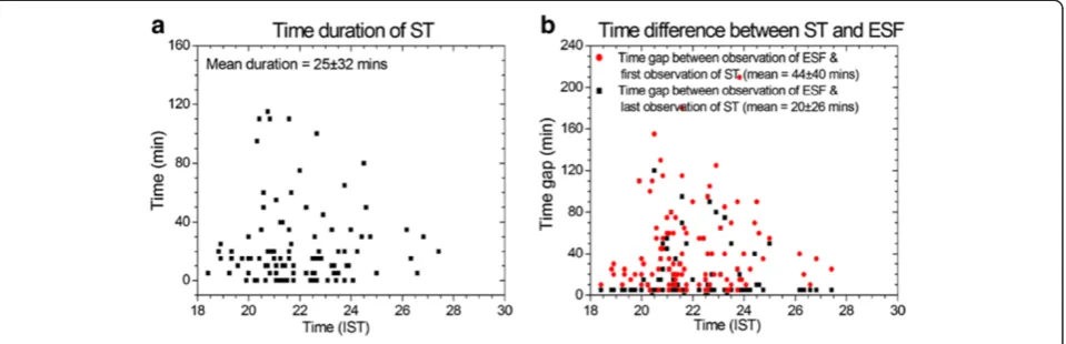
As mentioned above, 70% of events show the forma-tion of ESF after the occurrence of ST indicating that it is an important parameter in the generation of ESF. For considering ST as a precursor of ESF, it is important to understand how early ST appears before ESF onset. An average time delay between ST events and ESF is ob-tained here. Figure 11a shows the duration of ST events with IST. If ST is noticed in only one ionogram, its dur-ation is represented as 0 min. If ST occurs in more num-ber of ionograms (at 5-min intervals), the duration is
Figure 11Duration of ST (a) and time delays between ST occurrences and observations of ESF (b).
taken as the time difference between the last and first occurrences. Figure 11a reveals that the average ST dur-ation was about 25 min. The median value of 15 min indicates that the ST in general lasted for approximately 15 min.
Figure 11b shows the time delays (i) between the first occurrence of ST and the first occurrence of ESF (red dots) and (ii) between the last occurrence of ST and the first occurrence of ESF (black dots). On the average, the ESF occurred about 44 min after the first occurrence of ST, with a median value of approximately 30 min. This implies that ST can be used as a potential precursor signature, with an average warning time of 30 min. Our results (Figure 11b) indicate that on about half of the cases ESF was observed immediately following the last occurrence of ST, while there is a time delay between the last occurrence of ST and the formation of ESF in the remaining cases.
It may be rightly argued that the formation of ESF also depends on several other parameters such as PRE. Re-cent satellite observations show that the vertical drift due to PRE is generally absent at satellite altitudes dur-ing the extended solar minimum period of the present study (Stoneback et al. 2011). A detailed investigation on the intensity of PRE (if present), altitudes, and electron density gradients in the bottomside ionosphere is under-way. Preliminary results relevant to the days with the occurrence of STs are discussed in the next section.
Role of PRE on the days with ST
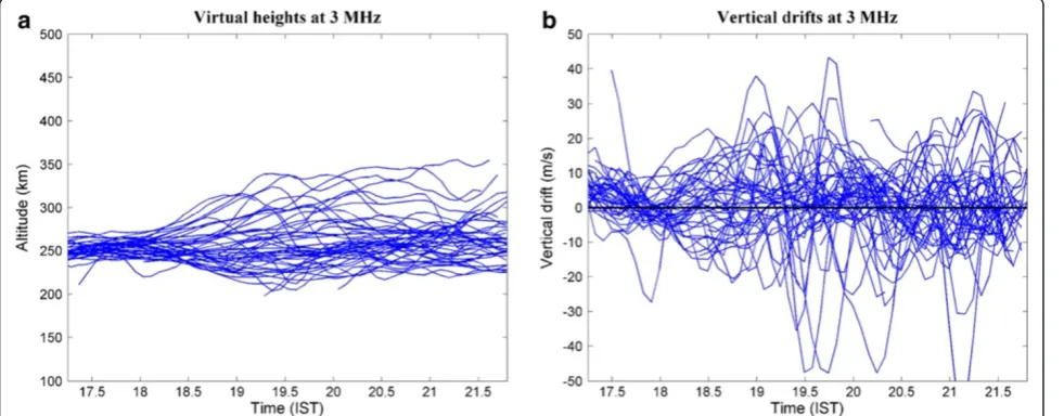
We found that all cases of ST observations do not lead to the formation of ESF, which may be due to unfavor-able background conditions. PRE is an important back-ground condition for ESF onset. Here, we analyze the
altitude of 3-MHz reflections and the corresponding vertical drifts during 18 to 22 IST for the nights when ST occurred before 22 IST. Figure 12a,b shows the virtual height of the 3-MHz reflections and the corresponding vertical drift estimated as rate of change of 3-MHz reflections, respectively, for the nights when there were STs before 22 IST but no ESF afterwards. As shown in Figure 12a, on most of the days, the altitude did not reveal the typical rise associated with PRE. The upward vertical drift (Figure 12b) was mostly less than 10 m/s and under-went positive/negative fluctuations, indicating the presence of oscillations in the bottomside ionosphere. Hence, no clear evidence seems to exist for strong PRE on these days.
Figure 13a,b is similar to Figure 12a,b, but for days when ST occurrence before 22 IST was followed by ESF. Surprisingly, the results are similar to the previous case (Figure 12) in which the signatures of PRE were absent on majority of the nights. Vertical drifts displayed in Figure 13b also indicate the existence of oscillatory features rather than persistent upward drifts. Both Figures 12 and 13 indicate that the PRE control on ESF was insignificant in the Indian sector during extended solar minimum period (or very low solar activity conditions). In the ab-sence of PRE, other background conditions such as bot-tomside density gradients may be important, which we plan to take up in future studies. The oscillations found in the bottomside ionosphere indicate that the existence of strong seed perturbations themselves may be sufficient for the onset and maintenance of bottomside ESF, which need detailed investigations.
Conclusions
The relationship between the occurrence of STs in iono-grams and the formation of ESF is studied using the
ionosonde observations made at 5-min intervals from an Indian dip equatorial station from March 2008 to February 2009 during the extended solar minimum conditions. The results reveal the following: (1) The zonally drifting ESF irregularities can be differentiated from those forming over the observing station. (2) Plasma blobs existing around the plasma depletions may be inferred from ionosonde mea-surements. (3) About 50% of the observed ESF events were preceded by ST. (4) ST occurred at later hours of the night as well implying that PRE is not the cause of ST at these hours. (5) STs were not followed by ESF in about 30% of the cases indicating that LSWS does not trigger ESF in all occasions. (6) About 70% of the STs were followed by ESF, and the percentage was high in sum-mer solstice and during later hours of the night. (7) Fol-lowing the occurrence of ST, the ESF onset was delayed by about 30 min on the average, indicating that ST may be used as a precursor of ESF. (8) PRE was almost non-existent in the Indian sector on most of the nights dur-ing the extended solar minimum.
Competing interests
The authors declare that they have no competing interests.
Authors’contributions
VLN carried out the major part of the analysis and wrote the manuscript. SS was involved in the remaining part of the data analysis. SG, KS, and NB contributed to the interpretation and organization of the paper. KE helped in the data acquisition and SSP participated in the discussions. All authors read and approved the final manuscript.
Acknowledgements
The lead author V. L. N. acknowledges the support from the National Institute of Information and Communications Technology, Japan under its International Exchange Program. The observations presented in this work were carried out by the Indian Institute of Geomagnetism with the support from the Department of Science and Technology, Government of India.
Author details
1
Solar-Terrestrial Environment Laboratory, Nagoya University, Furo-cho, Chikusa-ku, Nagoya, Aichi, 464-8601, Japan.2Present address: Indian Institute
of Science Education and Research Mohali, Sector 81, Manauli PO 140306, SAS Nagar, India.3Equatorial Geophysical Research Laboratory, Indian
Institute of Geomagnetism, Krishnapuram, Tirunelveli 627011, India.4Indian Institute of Geomagnetism, Plot 5, Sector 18, New Panvel, Navi Mumbai 410218, India.
Received: 30 April 2014 Accepted: 14 November 2014
References
Abdu MA, Batista IS, Bittencourt JA (1981) Some characteristics of spread F at the magnetic equatorial station Fortaleza. J Geophys Res 86:6836–6842 Abdu MA, de Medeiros RT, Bittencourt JA, Batista IS (1983) Vertical ionization drift
velocities and range type spread F in the evening equatorial ionosphere. J Geophys Res 88:399–402
Abdu MA, Kherani EA, Batista IS, de Paula ER, Fritts DC, Sobral JHA (2009) Gravity wave initiation of equatorial spread F/plasma bubble irregularities based on observational data from the SpreadFEx campaign. Ann Geophys 27:2607–2622
Abdu MA, Batista IS, Reinisch BW, MacDougall JW, Kherani EA, Sobral JHA (2012) Equatorial range spread F echoes from coherent backscatter, and irregularity growth processes, from conjugate point digital ionograms. Radio Sci 47, RS6003, doi:10.1029/2012RS005002
Abdu MA, Kherani EA, Batista IS, Reinisch BW, Sobral JHA (2014) Equatorial spread F initiation and growth from satellite traces as revealed from conjugate point observations in Brazil. J Geophys Res 119:1–9, doi:10.1002/2013JA019352 Aggson TL, Laakso H, Maynard NC, Pfaff RF (1996) In situ observations of
bifurcation of equatorial ionospheric plasma depletions. J Geophys Res 101:5125–5132
Balachandran Nair R, Balan N, Bailey GJ, Rao PB (1992) Spectra of the AC electric fields in the post-sunset F-region at the magnetic equator. Planet Space Sci 40:655–662
Basu S, Basu S (1981) Equatorial scintillations–a review. J Atmos Terr Phys 43:473–489
Booker HG, Wells HW (1938) Scattering of radio waves by the F-region of the ionosphere. Terr Magn Atmos Electr 43:249–256
Calvert W, Cohen R (1961) The interpretation and synthesis of certain spread-F configurations appearing on equatorial ionograms. J Geophys Res 66:3125–3140
Chapagain NP, Fisher DJ, Meriwether JW, Chau JL, Makela JJ (2013) Comparison of zonal neutral winds with equatorial plasma bubble and plasma drift velocities. J Geophys Res 118:1802–1812, doi:10.1002/jgra.50238 Fagundes PR, Bittencourt JA, de Abreu AJ, Moor LP, Muella MTAH, Sahai Y,
Abalde JR, Pezzopane M, Sobral JHA, Abdu MA, Pimenta AA, Amorim DCM (2012) A typical nighttime spread-F structure observed near the southern crest of the ionospheric equatorial ionization anomaly. J Geophys Res 117, A04308, doi:10.1029/2011JA017118
Farley DT, Balsley BB, Woodman RF, McClure JP (1970) Equatorial spread F: implications of VHF radar observations. J Geophys Res 75:7199–7216 Fejer BG, Scherliess L, de Paula ER (1999) Effects of the vertical plasma drift
velocity on the generation and evolution of equatorial spread F. J Geophys Res 104:19859–19869
Huba JD, Ossakow SL, Joyce G, Krall J, England SL (2009) Three-dimensional equatorial spread F modeling: zonal neutral wind effects. Geophys Res Lett 36, L19106, doi:10.1029/2009GL040284
Jayachandran B, Balan N, Rao PB, Sastri JH, Bailey GJ (1993) HF Doppler and ionosonde observations of the onset conditions of equatorial spread F. J Geophys Res 98:13741–13750
Kelley MC, Maruyama T (1992) A diagnostic model for equatorial spread F. 2. The effect of magnetic activity. J Geophys Res 97:1271–1277
Kelley MC, Larsen MF, LaHoz C (1981) Gravity wave initiation of equatorial spread F–a case study. J Geophys Res 86:9087–9100
King GAM (1970) Spread F on ionograms. J Atmos Terr Phys 32:209–212 Kudeki E, Bhattacharyya S (1999) Postsunset vortex in equatorial F-region
plasma drifts and implications for bottomside spread-F. J Geophys Res 104:28163–28170
Le G, Huang CS, Pfaff RF, Yeh HC, Heelis RA, Rich FJ, Harison M (2003) Plasma density enhancements associated with equatorial spread F: ROCSAT-1 and DMSP observations. J Geophys Res 108:1318, doi:10.1029/2002JA009592 Li G, Ning B, Abdu MA, Wan W, Hu L (2012) Precursor signatures and evolution
of post-sunset equatorial spread-F observed over Sanya. J Geophys Res 117, A08321, doi:10.1029/2012JA017820
Lynn KJ, Otsuka Y, Shiokawa K (2011) Simultaneous observations at Darwin of equatorial bubbles by ionosonde-based range/time displays and airglow imaging. Geophys Res Lett 38, L23101, doi:101029/2011GL049856 Lynn KJW, Otsuka Y, Shiokawa K (2013) Ionogram-based range-time displays for
observing relationships between ionosonde satellite traces, spread F and drifting optical plasma depletions. J Atmos Sol-Terr Phys 98:105–112 Lyon AJ, Skinner NJ, Wright RW (1961) Equatorial spread-F at Ibadan, Nigeria.
J Atmos Terr Phys 21:100–119
Maruyama T, Matuura N (1984) Longitudinal variability of annual changes in activity of equatorial spread F and plasma bubbles. J Geophys Res 89:10903–10912
Narayanan VL, Taori A, Patra AK, Emperumal K, Gurubaran S (2012) On the importance of wave-like structures in the occurrence of equatorial plasma bubbles: a case study. J Geophys Res 117, A01306, doi:10.1029/2011JA017054 Ossakow SL, Chaturvedi PK (1978) Morphological studies of rising equatorial
spread F bubbles. J Geophys Res 83:2085–2090
Park J, Min KW, Lee JJ, Kil H, Kim VP, Kim HJ, Lee E, Lee DY (2003) Plasma blob events observed by KOMPSAT-1 and DMSP F15 in the low latitude nighttime upper ionosphere. Geophys Res Lett 30:2114, doi:10.1029/2003GL018249 Park J, Noja M, Stolle C, Luhr H (2013) The ionospheric bubble index deduced
Patra AK, Taori A, Chaitanya PP, Sripathi S (2013) Direct detection of wavelike spatial structure at the bottom of the F region and its role on the formation of equatorial plasma bubble. J Geophys Res 118:1196–1202, doi:10.1002/ jgra.50148
Piggott WR, Rawer K (1978) U.R.S.I. handbook of ionogram interpretation and reduction. World Data Center A for Solar-Terrestrial Physics, Boulder Pimenta AA, Sahai Y, Bittencourt JA, Abdu MA, Takahashi H, Taylor MJ (2004)
Plasma blobs observed by ground-based optical and radio techniques in the Brazilian tropical sector. Geophys Res Lett 31, L12810, doi:10.1029/ 2004GL020233
Prakash S, Pal S, Chandra H (1991) In-situ studies of equatorial spread-F over SHAR–steep gradients in the bottomside F-region and transitional wavelength results. J Atmos Terr Phys 53:977–986
Rastogi RG (1977) Equatorial range spread F and high multiple echoes from the F region. Proc Indian Acad Sci 85:230–235
Sastri JH, Sasidharan K, Subramanyam V, Rao MS (1979) Range and frequency spread-F at Kodaikanal. Ann Geophys 35:153–158
Sekar R, Suhasini R, Raghavarao R (1994) Effects of vertical winds and electric fields in the nonlinear evolution of equatorial spread F. J Geophys Res 99:2205–2213
Sripathi S, Kakad B, Bhattacharyya A (2011) Study of equinoctical asymmetry in the equatorial spread F (ESF) irregularities over Indian region using multi-instrument observations in the descending phase of solar cycle 23. J
Geophys Res 116, A11302, doi:10.1029/2011JA016625
Stoneback RA, Heelis RA, Burrell AG, Coley WR, Fejer BG, Pacheco E (2011) Observations of quiet time vertical ion drift in the equatorial ionosphere during the solar minimum period of 2009. J Geophys Res 116, A12327, doi:10.1029/2011JA016712
Takahashi H, Taylor MJ, Pautet P-D, Medeiros AF, Gobbi D, Wrasse CM, Fechine J, Abdu MA, Batista IS, Paula E, Sobral JHA, Arruda D, Vadas SL, Sabbas FS, Fritts DC (2009) Simultaneous observation of ionospheric plasma bubbles and mesospheric gravity waves during the SpreadFEx campaign. Ann Geophys 27:1477–1487
Thampi SV, Yamamoto M, Tsunoda RT, Otsuka Y, Tsugawa T, Uemoto J, Ishii M (2009) First observations of large-scale wave structure and equatorial spread F using CERTO radio beacon on the C/NOFS satellite. Geophys Res Lett 36, L18111, doi:10.1029/2009GL039887
Thampi SV, Tsunoda RT, Jose L, Pant TK (2012) Ionogram signatures of large-scale wave structure and their relation to equatorial spread F. J Geophys Res 117, A08314, doi:10.1029/2012JA017592
Tsunoda RT (1985) Control of the seasonal and longitudinal occurrence of equatorial scintillations by the longitudinal gradient in integrated E region Pedersen conductivity. J Geophys Res 90:447–456
Tsunoda RT (2005) On the enigma of day-to-day variability in equatorial spread F. Geophys Res Lett 32, L08103, doi:10.1029/2005GL022512
Tsunoda RT (2008) Satellite traces: an ionogram signature for large-scale wave structure and a precursor for equatorial spread F. Geophys Res Lett 35, L20110, doi:10.1029/2008GL035706
Tsunoda RT (2010) On equatorial spread F: establishing a seeding hypothesis. J Geophys Res 115, A12303, doi:10.1029/2010JA015564
Tsunoda RT (2012) A simple model to relate ionogram signatures to large-scale wave structure. Geophys Res Lett 39, L18107, doi:10.1029/2012GL053179 Valladares CE, Villalobos J, Sheehan R, Hagan MP (2004) Latitudinal extension of
low-latitude scintillations measured with a network of GPS receivers. Ann Geophys 22:3155–3175
Weber EJ, Buchau J, Eather RH, Mende SB (1978) North–south aligned equatorial airglow depletions. J Geophys Res 83:712–716
Woodman RF, LaHoz C (1976) Radar observations of F region equatorial irregularities. J Geophys Res 81:5447–5466
Wright JW, Argo PE, Pitteway MLV (1996) On the radiophysics and geophysics of ionogram spread F. Radio Sci 31:349–366
Zalesak ST, Ossakow SL, Chaturvedi PK (1982) Nonlinear equatorial spread F: the effect of neutral winds and background Pedersen conductivity. J Geophys Res 87:151–166
doi:10.1186/s40623-014-0160-4
Cite this article as:Narayananet al.:A statistical study of satellite traces and evolution of equatorial spread F.Earth, Planets and Space 201466:160.
Submit your manuscript to a
journal and benefi t from:
7Convenient online submission
7Rigorous peer review
7Immediate publication on acceptance
7Open access: articles freely available online
7High visibility within the fi eld
7Retaining the copyright to your article