University of Windsor University of Windsor
Scholarship at UWindsor
Scholarship at UWindsor
Electronic Theses and Dissertations Theses, Dissertations, and Major Papers
2016
Research and Development of an Advanced RFID Security System
Research and Development of an Advanced RFID Security System
Based on Locating Multiple Tags
Based on Locating Multiple Tags
Lakhbir Singh University of Windsor
Follow this and additional works at: https://scholar.uwindsor.ca/etd
Recommended Citation Recommended Citation
Singh, Lakhbir, "Research and Development of an Advanced RFID Security System Based on Locating Multiple Tags" (2016). Electronic Theses and Dissertations. 5764.
https://scholar.uwindsor.ca/etd/5764
This online database contains the full-text of PhD dissertations and Masters’ theses of University of Windsor students from 1954 forward. These documents are made available for personal study and research purposes only, in accordance with the Canadian Copyright Act and the Creative Commons license—CC BY-NC-ND (Attribution, Non-Commercial, No Derivative Works). Under this license, works must always be attributed to the copyright holder (original author), cannot be used for any commercial purposes, and may not be altered. Any other use would require the permission of the copyright holder. Students may inquire about withdrawing their dissertation and/or thesis from this database. For additional inquiries, please contact the repository administrator via email
Research and Development of an Advanced RFID Security System Based on Locating Multiple Tags
By
LAKHBIR SINGH
A Thesis
Submitted to the Faculty of Graduate Studies through the
Department of Electrical and Computer Engineering in Partial Fulfillment
of the Requirements for the Degree of Master of Applied Science at
The University of Windsor
Windsor, Ontario, Canada
© 2016 LAKHBIR SINGH
All Rights Reserved. No Part of this document may be reproduced, stored or otherwise retained in a retrieval system or transmitted in any form, on any
Research and Development of an Advanced RFID Security System Based on Locating Multiple Tags
By
Lakhbir Singh
APPROVED BY:
______________________________________________ Dr. Wladyslaw Kedzierski, External Reader
Department of Physics
______________________________________________ Dr. Huapeng Wu, Department Reader
Department of Electrical and Computer Engineering
______________________________________________ Dr. Roman Gr. Maev, Advisor
Department of Electrical and Computer Engineering/Physics
AUTHOR’S DECLARATION OF ORIGINALITY
I hereby certify that I am the sole author of this thesis and that no part of this thesis has been published or submitted for publication.
I certify that, to the best of my knowledge, my thesis does not infringe upon anyone’s copyright nor violate any proprietary rights and that any ideas, techniques, quotations, or any other material from the work of other people included in my thesis, published or otherwise, are fully acknowledged in accordance with the standard referencing practices. Furthermore, to the extent that I have included copyrighted material that surpasses the bounds of fair dealing within the meaning of the Canada Copyright Act, I certify that I have obtained a written permission from the copyright owner(s) to include such material(s) (if any) in my thesis and have included copies of such copyright clearances to my appendix.
ABSTRACT
Radio Frequency Identification (RFID) has gained a lot of attention lately with the introduction of RFID tags or inlays for a variety of applications. Most common is location tracking which can further be used for detecting the movements of tags from their original positions. In order to develop a system for finding the change in tag positions, a correct combination of RFID tags and reader is vital. Also, better understanding of challenges facing the RF signal can be productive. Environmental factors, antenna radiation pattern and orientation are some key issues, which can undermine this approach. In this thesis, to address some of the challenges a security
algorithm for indoor RFID systems is proposed for detecting the change in the tag positions by finding the change in inter-tag distance. Also, several measures have been used to overcome the random nature of the RF signal. Experiments and evaluation of the above-mentioned methods in real time prove the robustness of the techniques considered for providing security.
DEDICATION
To my loving family:
Father: Surinder Singh
ACKNOWLEDGEMENTS
I would like to thank my supervisor Dr. Roman Gr. Maev for giving me the opportunity to work with him to obtain my degree. I need to thank him for all of the guidance, advice, support, and encouragement he has given me throughout my research.
I would like to thank Dr. Huapeng Wu and Dr. Wladyslaw Kedzierski for agreeing to be a part of my committee and contributing their time from their busy schedules.
I need to thank IDIR labs and its team for their continuous support and encouragement throughout my university career that has allowed me to pursue my interests.
TABLE OF CONTENTS
AUTHOR’S DECLARATION OF ORIGINALITY ... iv
ABSTRACT………v
DEDICATION ... ... vi
ACKNOWLEDGEMENTS ... vii
LIST OF TABLES ... ... x
LIST OF FIGURES ... ... xi
LIST OF ABBREVIATIONS ... xiv
1. Chapter 1-INTRODUCTION ... 1
1.1. Thesis Objective. ... ... 4
1.1.1. Research Goals .. ... 4
1.2. Thesis Outline ... ... 5
2. Chapter 2-BACKGROUND AND RELATED THEORY ... 6
2.1. Radio Frequency Identification (RFID) Technology ... 6
2.2. RFID System ... ... 8
2.2.1. RFID Tag ... ... 9
2.2.2. Types of RFID Tag ... 11
2.2.3. Tag Properties ... ... 13
2.2.4. RFID Reader ... ... 16
2.2.5. Tag and Reader Specifications Used for this Research ... 19
2.3. Antenna ... ... 21
2.3.1 Introduction To Antenna ... 21
2.3.2 Types of Antenna ... 23
2.3.3 Antenna Specification Used for RFID System ... 26
3.1. Overview ... ... 31
3.2. Indoor Propagation Model for Far Field Passive RFID System ... 33
3.3. Trilateration ... ... 36
3.4. Optimization for Nonlinear Systems ... 37
3.5. Interquartile Range .... ... 38
3.6. Adaptive Kalman Filter ... 39
3.7. Relative Error ... ... 45
4. Chapter 4-EXPERIMENTAL RESULTS ... 46
4.1. Indoor Large Scale Propagation Model Results ... 46
4.2. Adaptive Kalman Filter Results ... 55
4.3. Relative Error Results ... 60
4.4. Results Summary ... ... 67
5. Chapter 5-CONCLUSION AND FUTURE WORKS………….……68
5.1. Conclusion ... ... 68
5.2. Future works ... ... 69
REFERENCES ... ... 71
APPENDIX A: SIGNAL LEVEL MEASUREMENT CODE ... 75
APPENDIX B: SIGNAL LEVEL-DISTANCE CONVERSION CODE 96 APPENDIX C: OPTIMIZATION FOR FINDING INITIAL COORDINATES CODE ... ... 98
APPENDIX D: INTERQUARTILE RANGE CODE ... 100
APPENDIX E: ADAPTIVE KALMAN FILTER CODE ... 101
APPENDIX F: OPTIMIZATION FOR FINDING INTER-TAG DISTANCE AFTER FILTERING CODE ... 103
LIST OF TABLES
Table 4.1: Tolerance range of relative error for a Distance interval ... 62
LIST OF FIGURES
Figure 1.1: RFID system used in research ... 3
Figure 2.1: Magnetic field around a Wire/Coil ... 6
Figure 2.2: General diagram of RFID System ... 8
Figure 2.3: Block diagram of RFID Tag ... 10
Figure 2.4: Block diagrams for Active, Semi passive, and Passive tag [3] .. 12
Figure 2.5: Basic format for Electronic Product Code (EPC) [2] ... 14
Figure 2.6: Basic format for EPC Memory [7] ... 16
Figure 2.7: General block diagram of RFID reader components ... 17
Figure 2.8: Smartrac short dipole 273_2 UHF passive RFID tag [9] ... 20
Figure 2.9: Motorola MC3190-Z UHF active RFID reader [10] ... 20
Figure 2.10: Short dipole of length L [14] ... 27
Figure 2.11: Radiation pattern for short dipole antenna [14] ... 29
Figure 3.1: Block diagram of the security algorithm for indoor RFID system ... 32
Figure 3.2: Reader-Tag combination for measuring signal level for separate distances ... 33
Figure 3.3: Trilateration in two-dimensions ... 36
Figure 3.4: Block description of Interquartile Range ... 39
Figure 3.5: Block diagram of Adaptive Kalman Filter [16][19] ... 41
Figure 3.6: Trilateration in 2-dimensional with new coordinates ... 44
Figure 4.1: Estimated vs Actual distance graph for Tag T! at Location 1 .... 47
Figure 4.2: Estimated vs Actual distance graph for Tag T! at Location 1 .... 48
Figure 4.3: Estimated vs Actual distance graph for Tag T! at Location 2 .... 48
Figure 4.6: Estimated vs Actual distance graph for Tag T! at Location 3 .... 50 Figure 4.7: Estimated vs Actual distance graph for Tag T! at Location 4 .... 50 Figure 4.8: Estimated vs Actual distance graph for Tag T! at Location 4 .... 51 Figure 4.9: Target-reader coordinate diagram ... 52 Figure 4.10: Boxplot for E!" ... 53 Figure 4.11: Boxplot for E!" ... 54
LIST OF ABBREVIATIONS
ARAT Active Reader Active Tag
ARPT Active Reader Passive Tag
CRC Cyclic Redundancy Check
dBi Decibels Relative to Isotropic Antenna
dBm Decibel-milliwatt
EM Electromagnetic
EPC Electronic Product Code
FT. Feet
GEN-2 Generation-2
GPS Global Positioning System
HF High Frequency
IC Integrated Circuit
ID Identification
IQR Interquartile Range
LF Low Frequency
NFC Near Field Communications
PC Protocol Control Word
PCB Printed Circuit Board
PIFA Planar Inverted-F Antenna
PRAT Passive Reader Active Tag
RCPI Received Channel Power Indicator
RF Radio Frequency
RFID Radio Frequency Identification
RSSI Receive Signal Strength Indicator
TDS Tag Data Standard
TID Tag Identification
Chapter 1 INTRODUCTION
In today’s world, technology is growing rapidly and becoming necessary in our day-to-day lives. Our dependence on technology in every aspect of our lives has made our life easier and less complicated; Radio Frequency Identification (RFID) is one of the available technologies, which plays a significant role in helping to achieve this.
RFID is the use of radio waves to uniquely identify an object, item or person. This RFID technology gives birth to RFID tags or inlays, which represent a thin wire and a chip circuit, used to read and capture information from an EM source, typically a reader. This combination of RFID tag and reader is the simplest RFID system. The RFID system has been widely adopted as an attractive technology due to its low cost and its high technical capabilities. It has often been used in applications such as asset tracking, industrial automation, supply chain, automatic payments, and homecare and healthcare systems.
One of the most attractive applications of RFID is location tracking. A lot of research has been done in this area and different solutions have been proposed over the years using approaches like RSS- (Received signal strength) based technique, Time-based technique, and Phase-based
technique. These techniques can also be used for finding inter-tag distance in case where more than one tag being used. Likewise, different combinations of RFID tags and readers have been used to achieve tag location estimation and inter-tag distance with different types of RFID tags (explained in section 2.2.1 in detail).
need for using an RFID tag originated from the need to provide security. Placing tags at different positions on the painting and storing each tag’s Electronic Product Code (EPC), as explained in section 2.2.3 in detail, in a database cannot solve all security problems because a forger can use the same tags and place them at the same positions on a fake painting. The fake painting is then identified as a real one because the EPC of the tags attached to the painting is same with the EPC of the tags in database. While placing the tags acquired from original painting on to a fake one, a forger can easily alter the tags positions. Therefore, an interactive security system was needed such that we can detect the positions of the tags attached to the painting and any movement in their positions can be detected, thereby predicting the painting’s authenticity. The RFID system with two tags and a reader gives us a possibility of achieving the goal of this research.
This research includes the RFID system, which is comprised of two Ultra-High frequency (UHF) passive RFID tags with UHF passive Hand held RFID reader. The RSS-based technique is preferred over phase- and time-based technique because it is not possible for a handheld device to have a constant phase due to its continuous movement. Moreover, EM waves travel at the speed of light and hence it is difficult to detect accurate time taken by wave from sender to receiver. The RSS technique used in this
original positions or change in inter-tag distance if considering two tags in an RFID system, as in this case.
The reason for using two tags is simply because it is very easy for a forger to replace one tag and placed on to a fake painting precisely. Moreover, it is not very easy to detect change in the position of a single tag. Movement in the positions of the tags used in the RFID system from their original
positions will change their inter-tag distance. Therefore, by using two tags, and finding the change in their inter-tag distance can fulfill the requirement of achieving the research objective. UHF passive RFID tags are used due to their low cost, larger life span, and faster data transfer than other available tags in the market.
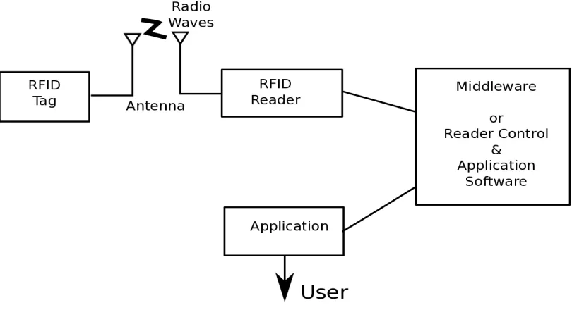
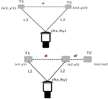
Figure 1.1 shows an RFID system taken into consideration in which two UHF passive RFID tags are placed at some position x!,y! and x!,y! in two-dimensional space with a UHF passive RFID reader at R!,R! . dis the
distance from center of tag T! to center of tag T!; L! is the distance between reader and tag T!; L! is the distance between reader and tag T!. If any change occurs in the positions of tags T! from x!,y! to nx!,ny! and similarly with tag T!, distance d between tags will change. This system is not limited to painting authentication but can also be used in applications such as
locating multiple moving tags in multi-storing building, used for autistic patient in a hospital for access control, used for providing security to items in museums and auction stores, can also be used in industrial automation for controlling equipment maneuvers, and other applications where any sort of security or control is required.
1.1 Thesis Objective
The main purpose of this research is:
• To develop an advanced RFID security system by detecting the
change in the positions of tags from their original positions. Any change occurs to the positions of the tags will change the inter-tag distance which ultimately changes the detectable parameters and therefore giving us a measure of predicting the movement in tags positions.
1.1.1 Research Goals
• Develop a smart device windows application (using c# programming
• Perform signal level-distance conversion for finding the distances between reader and tags.
• Finding the coordinates of vertices formed by reader and tags in an RFID system by means of nonlinear least-squares optimization, solving the system of nonlinear equations (using Matlab).
• Applying signal-processing measures for improving the location accuracy by designing adaptive Kalman filter (using Matlab).
• Determine the change in distance between the tags from their original positions by finding the change in relative error of inter-tag distance.
1.2 Thesis Outline
This section briefly explains the topic included in this thesis. In chapter 1, thesis introduction, thesis objective, and research goals are given. In chapter 2, background information is presented on RFID technology, RFID system, RFID tag and reader with their types, antenna and its basics, system
Chapter 2 BACKGROUND AND RELATED THEORY
There has been much research done in the area of RFID for locating tags and its use for security. This chapter focuses on giving an overview of RFID Technology. It then goes on to explain RFID Tags, RFID Reader, Antenna Basics and its popular types and the specification that is used in this
Research. The Tag and Reader specification for RFID system are also outlined in detail.
2.1 Radio Frequency Identification (RFID) Technology
In order to explain RFID, we need to understand radio waves. Radio waves are produced when free electrons oscillate in a wire. Electric current is produced in the wire with flow of electrons, which builds electromagnetic field around it. This field sends a wave outward whenever current is changing in the wire. If this methodology proceeds again and again for a period of time, an arrangement of waves is propagated at a discrete
frequency, which is nothing but radio waves. Figure 2.1 shows the magnetic field around a wire with constant electric current.
RFID means Radio Frequency identification and is a technique used for the purposes of automatic identifying, tracking, and validating the status,
authenticating tags using radio waves.
RFID technology existed for decades and its attaches can be followed down to World War II. For quite a while, RFID might have been utilized to planning radar to track planes, which might have been utilized by numerous nations in that duration of the time [1]. Developments over RF interchanges proceeded through 1950s. In 1960s, scholars and researchers from
everywhere throughout the globe published papers viewing RF signal
utilization to remote article ID number. In year 1973, first U.S. patent for an active RFID with rewriteable memory was believed to be gain by Mario W. Cardullo [1]. Charles Walton gained a patent for passive transponder in the same quite a while [1]. In mid-1980s, RFID tags been produced by different associations for business purposes. A percentage of organizations afterward opted to low and high radio frequency transponders for quicker information exchange and amazing read and write range [1].
IBM particular architects created and protected an ultra-high frequency (UHF) RFID framework in early 1990s. However, IBM sold their patent with Intermec, a bar code service provider [1]. UHF system advertised more drawn out read range typically 20 feet under beneficial conditions and
speedier information exchange [1]. A breakthrough happened in RFID Technology in 1999 when two Massachusetts Institute of Technology
professors,David Brock and Sanjay Sarma [1] produced an inexpensive
introduction of second-generation standard of EPC in 2004 [1], use of EPC became very common and many organizations started utilizing EPC
approach for their business purposes. Today, the main applications of RFID are Security access control (automated tolling), Traffic
analysis/management, and Retail, Logistics and supply chain management, Antiques monitoring, Vehicle monitoring, and E-commerce.
2.2 RFID System
RFID system is a combination of RFID tags (Transponders) and reader or interrogator. The reader sends out the RF signal carrying commands to the tags and RFID tags responds with its stored data to be authorized, detected or counted. RFID tag and reader are discussed in detail later in this section. A general description of RFID system is given in the Figure 2.2.
There can be different combinations of RFID system based on the category of tag and reader, most common are given [2] below:
1) An active reader passive tag (ARPT): It is a system in which reader RF signal retrieves data from tag.
2) An active reader active tag (ARAT): It is a system in which tag continuously sends RF signal to reader.
3) A passive reader active tag (PRAT): It is a system in which tag emits radio waves with data to reader, which is then used for further
processing.
The ARPT framework used for this research utilizes two passive UHF RFID tags, which communicate with an active RFID reader.
2.2.1 RFID Tag
RFID Tags are tags, labels or inlays, which work on the principle of using radio waves to read and capture information. A typical RFID tag consists of transceiver antenna and integrated chip circuit as shown in Figure 2.3. Transceiver antenna acts as a transducer between EM field and electric energy [2] and is responsible for bidirectional interfacing. It extracts energy and data from input signal and feed them to the chip circuit.
received with commands and retrieves the information from the memory. Modulator performs digital to analog conversion with clock recovery after data processing.
Figure 2.3: Block diagram of RFID Tag
Backscatter modulation occurs for passive and semi passive tags
modulator, power generator feeds the antenna for transmitting. Return scattered signal is detected and decoded by reader.
2.2.2 Types of RFID Tags
Based on battery source and backscattering, we can categorize RFID tag into three types: Active, Semi passive, and Passive tags [3], which are outlined below one by one.
1) Active tag: Tags with its own power source (typically a battery) for tag circuitry and do not possess backscattering modulation, called as Active tags. These tags have capability of initiating communications because they are continuously sending signal, which can then be detected by a reader. Modulator serves the purpose for active transmitter. There are some advantages for active tags like longest range (typically up to 100 feet or more); maximum data transfer with some disadvantages like lifetime of 2 years (approx.), high cost etc. 2) Semi passive tag: Tags with a power source (Battery) for tag circuitry
and possess battery-assisted backscatter, called Semi Passive tags. These tags do not have active transmitter and hence rely on
backscattering for transmitting signal. They have battery lifetime of more than 5 years and read/write range as far as 100 feet (Typical). They are less expensive than active tags and hence preferred more today over active tags.
3) Passive tag: Tags, which do not have a battery, instead drive power from the radio waves sent by reader (Source) and possess
these tags have been used in all sectors and preferred over active and semi passive tags.
Figure 2.4: Block diagrams for Active, Semi passive, and Passive tag [3]
frequencies an RFID system might utilize. Generally, the most common [4] are
• Low frequency (LF), which is 125 – 134 kHz.
• High frequency (HF), which is 13.56 MHz.
• Ultra-high frequency (UHF), which is 433, and 860-960 MHz.
Hence different types of RFID tags can be named as LF, HF, and UHF Active, Semi passive or Passive RFID tag. Each type of RFID tag has its own advantages and limitations. Depending on the requirement, one can choose an appropriate tags and readers combination. Note that RFID tags and readers must be tuned to the same frequency in order to interact with each other despite frequency hopping is enabled.
2.2.3 Tag Properties
There are different properties or parameters that are associated with RFID tag, which are used by different organizations in a wide spectrum of
applications for achieving their respective goals. This section only focuses on properties which have been used in this research or which are of utmost importance such as Electronic product code (EPC), Memory bank, Protocol control word (PC bits), Received signal strength indicator (RSSI) or signal level.
distinct identifiers to identify tags at very high rates and at distances under the reader zone, without having direct line-of-sight
communication [5]. These aspects from claiming RFID could make leveraged to support supply chain perceivability and expand stock precision. Basic format for EPC is given below in Figure 2.5.
Header EPC Manager
Number
Object Class Serial
Number
80 8-bits
0437528 28-bits
300000 24-bits
00A103177 36-bits
Figure 2.5: Basic format for Electronic Product Code (EPC) [2]
EPC is divided into four different sections, which are given below as
• Header: It associates the length, type, structure, rendition and
era of the EPC. It need an 8-bit size and cannot be transformed. Here 80 represent the header (EPC Type) for RFID tag EPC [2].
• EPC Manager Number: It is answerable for administering the
following partitions as shown in Figure 2.5. It has a 28-bit size and is imprinted during manufacturing, hence irreversible. Here 0437528 represent EPC Manager Number (Manufacturer) for RFID tag EPC.
• Object Class: It identifies a class of an object or category of
irreversible after manufacturing of an RFID tag; 300000 represent Object Class (Product type) for RFID tag EPC.
• Serial Number: It identifies of instance, which can be alter or
change as per user convenience and has a size of 36-bits [2]. Due to the reversible feature of the code designated to serial number, serial number might be utilized to different security requisitions. 00A103177 represent Serial Number (Unique item) for RFID tag EPC.
Note that 80043752830000000A103177 is EPC of RFID tag.
2) Memory bank: RFID tag memory is divided into four parts: Reserved
memory, EPC memory, TID memory, and User memory [6] which are outlined below
• Reserved memory: This memory stores only kill password and
the access password (32 bits each) [6]. Kill password deactivate the tag and access password lock/unlock tag’s writing
capabilities. It holds just two codes and it will be just writable.
• EPC memory: Stores EPC code with 96 bits of writable
memory.
• TID memory: Contains the distinct tag ID number, and is
imprinted when IC is made. This part cannot be transformed.
• User memory: Stretched out memory, which might store
additional data when EPC segment memory is full. There will be no standard method for allocating this writable memory. 3) Protocol control word (PC bits): PC bits are incorporated inside the
(CRC) is allocated to word 0 and used to check error in the EPC memory [7]. Basic format for PC bits is given below in Figure 2.6.
CRC
Cyclic redundancy check (16 bits) Word 0
PC bits Word 1
EPC Data Word 2
EPC Data Word N
Figure 2.6: Basic format for EPC Memory [7]
4) Received signal strength indicator (RSSI): It is the measurement of power present in received radio waves. It is often measured in
Decibels-milliwatts (dBm) or in simply watts. RSSI can be expressed as a negative, zero, and positive value. When RSSI is negative then values closer to zero indicate a stronger signal and when it is positive, larger values indicate a stronger signal. Some more modern chipsets utilized RSSI from 0 to 256 alternatively 0 to -127 yet majority of new chipsets utilize 0 to -100. RSSI is reinstated as RCPI (Received
channel control Indicator) when working with 802.11 wireless. This property is very important for this research point of view because RSSI is used for signal strength-distance conversion. RSSI can also be called as Signal Strength.
2.2.4 RFID Reader
(finding tags that satisfy certain criteria), and filtering tags [2], etc. It uses an attached antenna to capture data from tags. Figure 2.7 shows different
components involved in RFID reader. Once the information has been
received from RFID tag using reader through a connected antenna, it is then sent to middleware (or reader control and application software) [2], which basically connects user application with the information from the reader.
Figure 2.7: General block diagram of RFID reader components
RFID readers can be broadly categorized into two types: Active and Passive readers [8]. Active reader is one, which sends out RF signal to
or fixed reader. Both have their own advantages and limitations. Companies like Zebra, Siemens Motorola etc. manufacture this equipment.
There are various important components in an RFID reader. But the most important one is reader antenna, which is used to transmit and capture signal level. There are two types of antennas, which are generally used in RFID reader - linear and circular-polarized antennas [2]. Linear antennas are responsive to tag alignment, which rely on the tag angle or placement. Antennas that emit linear polarized waves bring long ranges, and large amounts of power that enable their signal to infiltrate through various materials to read tags. On the other hand, antennas that emit circular polarized waves are less responsive to tag alignment, but are capable of delivering as much power as linear antennas and may have difficulty in reading tags. RFID readers and their antennas communicate and work hand in hand with each to identify tags. Electrical current is changed into
electromagnetic waves by RFID reader, which are then transmitted into space for capturing by a tag antenna and changed over again to electrical current. An optimal RFID reader selection varies as per the requirement of the application and environment.
applications. On the other hand, the reader and tag antenna communicating in long-range applications for transferring information, data or energy uses the method of electromagnetic coupling. The read range to these requisitions is greater than 30 cm and can be up to several meters [2] and the vicinity of any dielectrics can debilitate the identification of the tags.
2.2.5 Tag and Reader Specifications used for this Research
This section discusses the kind of RFID tags and reader used in this research. RFID system used for this research has two UHF passive RFID tag and a hand held RFID reader. Complete specifications of RFID system
components involved are given below.
1) RFID tag specification: As two UHF passive RFID tags are used in this research, both of them are of same type. They belong to same Smartrac 273_2 EPC class-1 Gen-2 with Impinj Monza 4 Integrated circuit (IC) and a short dipole antenna of same length (93mm) [9]. They have an operating frequency from 860-960 MHz (902-928 MHz is allowed in North America), −40!c to 85!c of operating
Figure 2.8: Smartrac short dipole 273_2 UHF passive RFID tag [9]
2) RFID reader specification: A Motorola MC3190-Z UHF active RFID
Just like short dipole UHF passive RFID tag, it also has same applications in supply chain management, industrial automation, and asset tracking. Figure 2.9 shows hand held RFID reader.
2.3 Antenna
An antenna is a device which sends or receives electromagnetic waves. It translates electromagnetic waves acquired from space into electrical current in conductors or vice-versa, depending on whether the antenna acts as receiver or transmitter [11][12].
The pairing of electronics and electromagnetic waves is done by antennas working on both ends either receiver or transmitter. It is a significant
component of radio device [12]. In general, there is a relationship between antenna size and the frequency used by the antenna. An antenna size must have the right length for the frequency used but this is not a hard and fast rule for manufacturer [12] while making antennas. In fact, there are
contemporary antennas that work with more than one frequency as in case of hopping frequency, which prevents the signal from dropping.
Electromagnetic waves can be radiated and received by an antenna uniformly in all straight and perpendicular directions or likely in a specific direction [12]. It additionally incorporated extra components or surfaces with no electrical unit with the transmitter or receiver, which helps to adjust the electromagnetic waves into a ray or any chosen radiation patterns.
2.3.1 Introduction to Antenna
devices were part of the analysis that manifested the very process of conversion of electromagnetic waves [11].
In 1830s, Faraday performed the first experiment, which involved the coupling of electricity and magnetism and hence proved a definitive relationship between them [11]. He smoothly passed a magnet around the coils of a wire connected to a galvanometer and in moving the magnet; he was actually developing a time-varying magnetic field, which must have had a time-varying electric field (from Maxwell-Faraday equation). The
electromagnetic waves produced were detected by the galvanometer attached, when coil behave like a loop antenna [11] and therefore proved antenna’s functioning.
Antennas played a very important role in the World War II and later on, their utilization revolutionized and changed the life of an average person via radio and television broadcasting [11]. The popularity of antenna was so enormous that in the United States, there was at least one antenna at every house [11]. This booming market of antennas also helps auto industry to compete and eventually grow during the same period [11]. Due to the new advancements in technology in the early 21st century with the introduction of mobile phones has changed the whole idea of antenna numbers and their portability [11]. Research pertaining to antenna growth leads to the development of wireless communication systems, which has become an essential element of our day-to-day life. The new research trend in antenna technology involves extensive research on metamaterials (an artificial material which contains the properties of dielectric and magnetic constants, that might be at the same time negative which ultimately give rise to
make antennas size shorter for its effective use in individual remote correspondence devices such as mobile phones [11].
New developments in RFID devices suggest that we can have more than one antenna per object [11] and this number will rule antennas utilization in future. As an essential part of communication technologies field, antenna theory is of high importance for electrical and communication engineers.
2.3.2 Types of Antenna
Antenna is an essential part of a communication device which allow for remote communication between a number of separated electric circuits [12]. Antenna gain, aperture, directivity and bandwidth, polarization, effective length and resonance are the properties of antenna, which can be used for categorizing antennas. In this section, we will discuss popular antenna types with their subcategories.
1) Wire Antennas: A wire antenna is an elementary radio antenna, comprising of a conducting wire, which is half the length of the maximum wavelength of the antenna [12]. This wire is split in the middle, and a current source (transmitter) separates the two sections as shown in Figure 2.10 for short dipole wire antenna. These types of antennas are fed at the center and any transmission and reception of radio signal is done at the center [12]. Types of wire antennas are: short dipole antenna, dipole antenna, half wave dipoles, broadband dipoles, monopole antenna, folded dipole antenna, loop antenna, and cloverleaf antenna [12].
known as aerial antenna. They categorized into three types of antennas such as bow-tie antennas, log periodic antennas and log periodic array [12][13].
The first type, bow-tie antennas or butterfly cannot be fully classified as log periodic antennas but these antennas lay a good foundation for discussing the initial phase of log periodic antennas [12]. The second type, log periodic antennas are antennas which are developed to achieve a goal of possessing a broader bandwidth [12]. The achievable bandwidth is hypothetically interminable but the real bandwidth attained rely on factors such as how big is antenna structure which is used to measure the lower frequency limit and how accurate the smaller attributes are on the antenna which measures the upper frequency limit [12]. Third, log periodic array are used to work with large frequency band and can be characterized into active and passive regions [12].
3) Travelling wave antennas: An antenna in which the current
circulations are generated by waves of charges propagated in only one direction in the conductors [12]. These antennas are also known as progressive-wave antenna. These antennas are categorized into three types of antenna such as helical antennas, Yagi-Uda antennas and spiral antennas [12][13].
Helical antenna is an antenna that produces radiation along its own axis [12]. These antennas have a shape of corkscrew and are also classified as axial mode helical antennas. These antennas exhibit some properties about utilizing helix antenna, which would be wider
antenna design among others. Just like helix, these antennas also exhibit some properties about their utilization, which are
straightforward construction and have a high gain, which is typically above 10 dB, operating from HF to UHF bands, and typically have littler bandwidth [12][13]. The most common example of Yagi antenna is roof top antenna. And last, spiral antennas are antennas with substantial bandwidth capacity and have association with category of frequency independent antennas [12].
4) Aperture antennas: Aperture antennas are antennas that are typically created with the combination of metal walls and dielectric, frequently with ridges [12]. The leaning of radiation fields over the opening of the antenna is a way of measuring fields from these types of antennas [12]. At large distances, the radiated fields originate from the aperture fields, which is in contradiction with Huygens-Fresnel principle, which states that “every point on a given wavefront become the radiating sources from which a spherical wavelet is propagating and the resulting field intensity be found by superposition which generates the next wave front” [12]. Aperture antennas are divided into various categories such as slot antenna, cavity-backed slot antenna, inverted-f antenna, slotted waveguide antenna, horn antenna, vivaldi antenna, and telescopes antenna [12].
5) Reflector antennas: Reflector antennas are antennas, which typically operates when an inflated gain (in case of satellite transmission or reception) or a very restricted main ray (in case of secure
communication) is required [12]. There is a direct relationship
However, large reflectors are difficult to implement due to their substantial size as compared to wavelengths [12].
This antenna categorized into two types: corner reflector, and parabolic reflector. The first one, corner reflector is an antenna that enhances antenna directivity [12]. The second one is parabolic
reflector antenna, which is a most common reflector antenna. It is also known as satellite dish antenna [12].
6) Microstrip antennas: A microstrip antenna is a small band, extensive antenna created by engraving the antenna component designs in metal outline attached to an insulating dielectric substrate, for instances a printed circuit board (PCB), with a constant metal layer connected to the inverse side of the substrate that layout a ground plane [12]. These antennas are also known as patch antennas. There are various standard shapes for microstrip antenna, which are square, rectangular, circular, and elliptical. Moreover, the feasibility of any continuous shape also exists [12]. Microstrip or patch antennas are getting to be
progressively functional on the account that they can be design or fabricated straight into a circuit board [12]. In fact, mobile phone industry is making an extensive use of microstrip antennas due to their smaller shape, lesser expense, and smoothly created capability [12]. Microstrip antennas can be categorized into two types: rectangular microstrip antennas, and planar inverted-f Antennas or PIFA microstrip antennas [12].
2.3.3 Antenna Specification used for RFID System
passive RFID tags used, which belongs to same Smartrac 273_2 EPC class-1 Gen-2 with Impinj Monza 4 Integrated circuit (IC) and a short dipole
antenna of same length [9] and a RFID reader which has an integrated orientation insensitive antenna. Both antennas are described below in detail.
1) Short Dipole antenna: The short dipole antenna is a modest version of the popular dipole antenna. Short dipole antenna is an antenna, which is made up of two conducting wires connected to each other through a transmitter at the center [14] as shown in Figure 2.10. The meaning of short is smaller size of the antenna relative to wavelength and
typically, antenna size is less than one tenth of the wavelength i.e.
L < !"!
Figure 2.10: Short dipole of length L [14]
I z = I!(1−2 ∣ z∣ L )
(2.1)
Equation (2.1) shows that the current amplitude on the short dipole is inversely proportional to the length of the dipole which shows longer dipole will have less current. The electric and magnetic fields radiated from the short dipole antenna in the far field [12] are given by:
E! = jηβ I!Le !!!!
8πr sinθ
(2.2)
H∅ = E!
η
(2.3)
E! = H! =E∅ = H! =0 (2.4)
The exponential term e!!!! and sinθin equation (2.2) describes the phase variations and spatial variations of the wave with distance, respectively. The electric field E! and magnetic field H∅ given in equation (2.2) and (2.4) have finite values and are orthogonal as well as in-phase with each other in case of far field [12]. These fields propagate in the direction opposite from the antenna and are
perpendicular to the direction of propagation [12]. These fields act like a plane-wave in far field and their amount decreases by 1/r and power reduced [12] by:
P r ∝ 1 r!
(2.5)
• Radiation pattern: Radiation pattern is the change in the strength of the
radio waves as they propagate away from the antenna [12]. The variation in the radio waves strength can be easily detected in the far field, which depends upon waves angle of arrival [12]. Antennas do not have equal radiation distribution [15]. They have maximum radiation in the direction front of them and the area covering the
maximum radiation is called main lobe [12][15]. Similarly, other lobes are side lobes, which have less radiation, and one back lobe, which have more radiation than side lobes but less than main lobe [15]. For better accuracy and reliability, data collection for this research is done in the main lobe. Figure 2.11 shows the radiation pattern for short dipole having an elliptical shape and it resembles a doughnut shape in 3-D. Note that the current is maximum in center and least at the end of the antenna.
• Antenna Gain: Antenna gain is defined as the ratio of amount of
power radiated by an isotropic antenna to the amount of power radiated by the antenna [15]. Antenna gain is often used due to its ability of giving precise information about the actual power loss while transmitting and receiving it [15]. Antenna gain can also be expressed as the ratio of total radiated power P! to the total input power P!"
supplied to antenna multiplying with the directivity D [15] as given in equation (2.6). Antenna gain for short dipole used in the research is 1 dBi.
G= P! P!"D
(2.6)
• Polarization: RFID tags antennas used in this research support linear
polarization. Linear polarization is the propagation of waves totally in one plane [15]. It is further divided into horizontal polarization, which is having wave’s electric field parallel to the plane and vertical
polarization, which is having wave’s electric field perpendicular to the plane [15].
Chapter 3 PROPOSED SECURITY ALGORITHM FOR INDOOR RFID SYSTEM
This chapter explains the proposed security algorithm for detecting the change in the positions of UHF passive RFID tags for the indoor RFID system. Each step or method implemented in the algorithm is described below with a separate section in full detail.
3.1 Overview
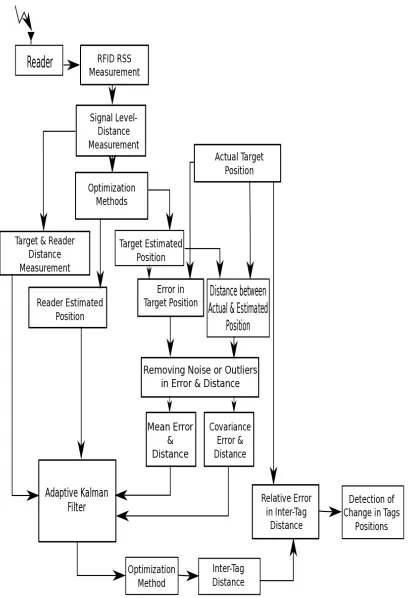
This section outlines the summary for the proposed security algorithm. This research is based on RSS-based technique [25][26] in which signal level is used to estimate the location of tags and then ultimately used to detect the change in location of tags. Further, any change in positions of tags can be detected by finding change in the relative error in inter-tag distance used in the RFID system. Figure 3.1 describes the general block diagram of the proposed security algorithm. A handheld RFID reader and two UHF passive RFID tags framework is used to achieve localization deployed in geometric composition by using the concept of trilateration in 2-dimensions to obtain unambiguous location. This model suffers from the variations of the signal level and those fluctuations come not only from the RF environment
[21][22], but also from the RFID antennas alignment and radiation pattern. In order to minimize the effect of those fluctuations, different signal
processing measures such as Interquartile Range, Adaptive Kalman Filter with optimization techniques for nonlinear systems at different stages of the algorithm are used to improve the location estimation. With the
improvement in location estimation, accuracy in inter-tag distance is also improved. Different measurements are taken at different distances for
at different distances is measured. A tolerance range is then obtained for indoor RFID system for a distance range, which will serve as the basis for this security system. Any change occurring in the positions of tags will make the relative error fall outside the tolerance range. Different methods used in this security algorithm are discussed below in detail.
3.2 Indoor Propagation Model for Far Field Passive RFID System
This section explains how to measure signal level using a c# windows application and then estimate the distance using the measured signal level. First it is necessary to measure signal level or received signal strength indicator (RSSI) from two tags using a handheld RFID reader at different distances for separate locations. Figure 3.2 shows two UHF tags with a RFID reader at different distance values D_1,D_2,…and D_n for measuring signal level for separate indoor locations.
A smart device windows application using c# programming language is designed to measure signal levels from the RFID tags in the reader’s coverage area. The code for measuring signal level is comprised of three windows forms in which the first form is the login page; the second form is the form for retrieving the list of items (or paintings) by selecting items by their categories from the database on which a security check is to be performed along with accessing the main database containing other information such as artist name, tag EPC, picture number etc.; the third form is the form for selecting the correct tags associated with the items used for the security check. As the basic idea for this research came from the authentication of paintings using RFID tags, this is the reason behind designing the windows form in this manner. It is possible to assign a picture number to the tags attached with it and store EPC in the database along with some other relevant information like Artist Name. By selecting a picture either by its picture number or artist name, a security check can be performed on the tags associated with selected items. In this way, it is possible to have an RFID system for security check without worry of other tags in the reader coverage area.
In order to perform signal level to distance conversion, an indoor large scale propagation model [16] is used. This model helps in finding tag location for a UHF passive RFID tag, which works on the principle of backscattering. In modulated backscatter scheme, the log-distance path loss in the RFID passive communication can be expressed [16] in the
following way:
PL d =P!!"#$ − P!!"#$ = PL d! +10 N log!" d
d!+X!
where
• PL d is the total path loss measured in Decibel (dB).
• P!!"#$ =10log!" !!!
!"# is the transmitted power in dBm, whereP!! is the transmitted power in watt.
• P!!"#$ =10log!" !!!
!"#is the received power in dBm, where P!! is the received power in watt.
• d!is an arbitrary reference distance in cm.
• d is the length of the path in cm.
• PL d! = 10log!"!!!
! is the path loss at the reference distance d! in Decibel(dB).
• !!!
! =
!"!! !
! !
!!!! !!!!! is ratio of power transmitted and received by
reader transmit and receive antennas.
• G!,g!,G!,g! are the gains of the reader a tag transmit and receive
antennas respectively.
• Γ is reflection coefficient of the tag.
• g!Γg! = !"#!!
• δ is radar cross-section of the RFID tag
• n is path loss exponent and N=2n for RFID passive communication.
• X! is zero mean Gaussian random variable with varianceσ!in dB, is
called shadow fading.
• λ is the wavelength in cm.
3.3 Trilateration
Trilateration is the process of relatively calculating the positions of points by taking these points as vertices of the triangle and utilizing the estimation of distances [17]. This process is used to have an unambiguous location of the tags in the RFID system using geometry. Figure 3.3 shows this process with tag T! at distance L! from the reader and its coordinates at the origin; a circle, representing possible location of the reader relative to this tag, can be drawn with tag T! as center and radius L!. Similarly, tag T! at distance L!
from the reader placed on the same axis i.e. x-axis in this case; a circle, representing possible location of the reader relative to this tag, can be drawn with tag T! as center with coordinates (d,0) and radius L! [31], where d is the distance between center of tag T! to the center of tag T!.
Figure 3.3: Trilateration in two-dimensions
Now, there are two points on the same x-axis with a distance d apart and two circles can be drawn with center and radius. The intersection of two circles represents the reader coordinates as shown in Figure 3.3 as (R!,R!).
In this process, there will be two points of intersection; both points are
3.4 Optimization for Nonlinear Systems
Optimization is a methodology, which finds the best of accessible results such that either the maximum or the minimum of the objective function is chosen via an appropriate algorithm. Using the geometry defined by trilateration, two tags can be placed on an object or item on the same axis with a reader at some point in space. First, with the help of distance measurement of tag T! from the reader and its coordinates at origin, the reader position (R!,R!) can be found by treating it as an optimization
problem with equation (3.2) as the objective function. Secondly, with the reader coordinates and the distance measurement of tag T! from the reader, the coordinates of target T! can also be estimated using optimization. By denoting the coordinates of the ith tag as (x!,y!) and length as L!, the
coordinates of the reader R!,R! can be estimated by solving the
optimization problem given in equation (3.2) using nonlinear least-squares
algorithm. Once the reader coordinates is estimated, target T! coordinates can also be estimated using the same technique with the same function given in equation (3.2) but with different length L!.
F(x,y) = (x!−R!)! + (y
!−R!)! −L! (3.2)
where
• F x,y is the objective function for optimization.
• (x!,y!)is the coordinates of ith tag
• R!,R! is the coordinates of the Reader
The same optimization method will be used in the later part of the algorithm once signal-processing measures is applied to find the new
coordinates of target, reader, and new distances between tags and the reader. Matlab is used for solving the problem of optimization and the results for this section can be found in section 4.1.
3.5 Interquartile range
Interquartile range (IQR) is basically used to detect an outlier or noisy data. It is a process, which can be used to measure the variability of a data set by partitioning them into quartiles [18]. Analyzed data are separated by their values into four parts referred to as quartiles; entities that partition each part are called the first, second, and third quartiles and are denoted by Q1, Q2, and Q3 [18]. They are also defined as 25 percentile, 50 percentile, and 75 percentile, respectively [18]. Figure 3.4 shows a block description of
interquartile range. The first quartile denoted by Q1 is median of values less than overall median; the second quartile denoted by Q2 is median of the data set; the third quartile denoted by Q3 is median of values greater than the overall median. Interquartile range can be measured mathematically by subtracting first quartile from the third quartile [18] as shown below:
IQR = 𝑄! −𝑄! (3.3)
An outlier can be removed from a data set by the standard criterion given below for Interquartile range (IQR) [18]:
criterion is applied to both the parameters defined above to remove a value (Outlier), which increases the variance of the whole dataset, which
ultimately increases the disturbance in the dataset. Both, error in target coordinates and the distance between actual and estimates target position will be used as a noise measurement or error in adaptive Kalman filter for producing better estimates of reader coordinates and distance between target and reader.
This method is basically used in this research to reduce the shadowing effect mentioned in section 3.2, as there is no specific value for this
parameter. The reason for applying this technique on the error and distance parameters instead on signal level is nothing but to remove the outliers, which can be a direct result of RF fluctuations [21] and statistical error. The results for this section can be found in section 4.1.
Figure 3.4: Block description of Interquartile Range
3.6 Adaptive Kalman Filter
processing. Kalman filtering has been utilized effectively for reducing signal noises and it demonstrates considerably high quality results in comparison to other types of filters. It is the one that minimizes the variation in the system [19]. It is used in applications like tracking the trajectory of the moving objects such as planes, ships, satellite etc. Kalman filtering can be utilized to reduce noise from an indoor RF signal for both moving and fixed devices. While applying Kalman filter to fixed location or devices, noise is assumed to be a function of time.
Figure 3.5 shows the general block diagram of an adaptive Kalman filter. Kalman filter can be divided into three models: Process model, Observation model, and new state [16].
1) Process model: This model explains the previous or initial state of the estimate and process covariance matrix or error in the estimate. The linear stochastic difference equation for a state of discrete-time controlled process for estimating a new state is [19] given by:
X!" = A∗x!!!+B∗u!+w! (3.5)
where
• x!!! is the previous state or initial state of the estimate.
• X!" is predicted state of the estimate.
• u! is the control variable matrix.
• w! is the predicted state noise matrix.
• A and B is the identity matrixes to avoid dimension mismatch.
As the tags are stationary, the state of the system is not modified with any control variable and the predicted state noise is also zero [16]. Thus the above equation can be written as:
Kalman filter is a function of noise; noise statistics is essential for achieving optimal filter output. Process noise in this case is very negligible as compared to measurement noise [16] because a
commercial handheld reader is used in this research. Therefore, the process covariance matrix given by equation (3.7) will assumed to be 1 [16]:
P!" = A∗P!!! ∗A! +Q
! (3.7)
where
• P!!! is process covariance matrix of previous state or initial state.
• Q! is process noise covariance matrix. Therefore
P!" =1 (3.8)
2) Observational Model: This model contributes towards finding the Kalman gain, which is used to find the new state of the estimate along with measurement inputs. Kalman gain [19] is defined by the equation (3.9):
K = P!"∗H
(H∗P!" ∗H! +R)
(3.9)
where
• P!" is the process covariance matrix.
• R is measurement noise covariance matrix.
• H is identity matrix.
Now, the most important part of Kalman gain is the measurement noise covariance matrix R. It is nothing but the error in target position and the distance between actual and estimated target position as
y! =c∗x!" +Z! (3.10) where
• x!" is new measurement.
• Z! is uncertainty in the measurement.
3) New or Updated state: This section outlines how a new or an updated state of estimate and process noise for an adaptive Kalman filter can be achieved. New or updated state can be defined mathematically [16] [19] by equation (3.11) and (3.12):
X! = X!" +K[y!−H∗X!" −u] (3.11)
P! = (I−K∗H)P!" (3.12)
where
• X!" is predicted state of the estimate.
• K is Kalman gain.
• y! is the measurement input.
• u is mean of the error in target coordinates and distance between
actual and estimated target coordinates explained in section 4.1.
• P!" is the predicted process noise.
• X! is the new state of estimate.
• P! is the new state of process noise or error in estimate.
estimates adapt or change with the error in target coordinates and distance between actual and estimated target coordinates, we defined Kalman filter as adaptive Kalman filter.
Adaptive Kalman filter gives us new estimates for the reader coordinates R!,R! , new estimate of the distance between target and reader and a new
estimate of the distance between new reader coordinates and tag T! as shown in Figure 3.6. In order to find new estimate of target coordinates or inter-tag distance, the nonlinear equation (3.13) can be solved by treating it as an optimization problem in the same way as explained in section 3.4.
Figure 3.6: Trilateration in 2-dimensional with new coordinates
F d! = NL!
! −NL ! ! +d
! !
2d! −NR!
(3.13)
where
• NL!is the new distance estimate between tag T! and reader
• NL! is the new distance estimate between tag T! and reader
• NR! is new x-coordinate estimate of reader.
• NR! is the new y-coordinate estimate of reader.
The results for this whole section can be found in section 4.2.
3.7 Relative Error
Relative error is defined as the ratio of difference between experimental and actual value and the actual value [20]. It is given in equation (3.14) as:
Relative error = x!"#!$%&!'()*−x!"#"!"$%"
x!"#"!"$%"
(3.14)
where
• x!"#!$%&!'()*is the new inter-tag distance estimate.
• x!"#"!"$%" is the actual distance between two tags or inter-tag distance.
Chapter 4 EXPERIMENTAL RESULTS
This chapter outlines the full description of experimental results and findings from this research. In this section, evaluation of the security algorithm for an indoor RFID system performance is given. It contains the results collected followed by their summary and interpretation.
4.1 Indoor Large Scale Propagation Model Results
This section addresses the results related to validation of Indoor Large Scale Propagation Model explained in section 3.2. All measurements were
recorded in the manner explained in section 3.2 from two UHF passive RFID tags used in the RFID system. A number of experimental sets were collected with a large number of individual measurements (about 250-550) within each. Each measurement was collected at different separation distance for separate indoor locations to perform signal level-distance conversion. Different distance is basically the actual distance between the tip of reader antenna and the center of two UHF passive tags. The smart device windows application using c# language is designed to capture the signal levels and their respective frequency from tags (full explanation of windows
application is given in section 3.2). The reader and tag antenna gains are 1.5dBi [10] and 1dBi respectively, reader antenna power for transmitting is 30dBm or 1 watt, radar cross section is considered to be 1cm!, path loss
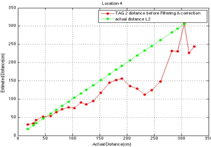
distance vs actual distance graph for two UHF passive tags at four different indoor locations is produced which depicts the estimated or calculated distance value from the indoor large scale propagation formula and the actual distance between reader and tags and given below from Figure 4.1 to 4.8. The reason for taking measurements at four different locations is
nothing but to check the behaviour of the RF signal level and how it changes with distances at different locations. The full c# code, which contributes towards measuring signal level, as described in section 3.2 can be found in Appendix A: Signal Level Measurement Code. The code for signal level to distance conversion is written in Matlab and can be found in Appendix B: Signal Level-Distance Conversion Code.
a) Location 1:
Figure 4.2: Estimated vs Actual distance graph for Tag T! at Location 1
b) Location 2:
Figure 4.4: Estimated vs Actual distance graph for Tag T! at Location 2
c) Location 3:
Figure 4.6: Estimated vs Actual distance graph for Tag T! at Location 3
d) Location 4:
Figure 4.8: Estimated vs Actual distance graph for Tag T! at Location 4
Now, trilateration techniques explained in section 3.3 can be applied to the system formed by the reader and tags. Using optimization explained in section 3.4 for non linear equations as given in equation (3.2), the
coordinates of reader R!,R! and the coordinates of the target which is tag
T! can be found with the help of estimated distance from the reader to tag T!
and T!. This process is repeated at different distances for each location dataset. The code for optimization is written in Matlab and can be found in Appendix C: Optimization for Finding Initial Coordinates Code.
the euclidean distance between estimated and actual target coordinates given in equation (4.2).
(E!",E!")= (d−d!"! ,0−d
!"
! ) (4.1)
D= (d−d!"! )!+ (0 −d
!"
! )! (4.2)
Where
• (d!"! ,d!"! ) is the estimated coordinates of target T!.
• (E!",E!")is the error coordinates of target T!.
• d is the x-coordinates of target or inter-tag distance.
• D is distance between actual and estimated target coordinates.
Figure 4.9 shows the error target coordinates with the actual target coordinates and reader coordinates. These coordinates values given in the Figure 4.9 are the mean values for location 1 dataset at a distance of 20 cm. Similarly, this process is repeated for all location at every distance.
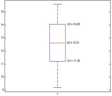
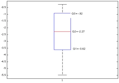
Once the coordinates from equation (4.1) and distance from equation (4.2) can be estimated, IQR criterion is applied on these dataset at every distance for each location. Figure 4.10 to 4.12 show the boxplot for the target error coordinates and the euclidean distance between actual and estimated target coordinates for location 1 dataset at a distance of 20 cm. Similarly, this process is repeated for all location at every distance. The results from this sample dataset states that the error data has no outlier or noise, which can increase the variance in the adaptive Kalman filter. The code for
Interquartile range (IQR) is written in Matlab and can be found in Appendix D: Interquartile Range Code.
Figure 4.11: Boxplot for E!"
4.2 Adaptive Kalman Filter Results
In this section, results processed with adaptive Kalman filter explained in section 3.6 are outlined. The error in target coordinates and the distance between estimated and actual target coordinates explained in section above would serve the purpose of reducing error from the target T! coordinates. Adjustment to the distance value between tag and reader can be made with respect to the covariance and the mean of the noise measurement. By considering all aspect and parameters mentioned in section 3.6, new filter estimates of distances between tags and reader are obtained. Given below are the estimated distance vs actual distance graphs from the same four indoors locations after filtering and correction is applied, which were considered for estimating distance in section 4.1. The code for Adaptive Kalman Filter is written in Matlab and can be found in Appendix E: Adaptive Kalman Filter Code.
a) Location 1:
Figure 4.14: Estimated vs Actual distance graph for Tag T! at Location 1 after filtering
b) Location 2:
Figure 4.16: Estimated vs Actual distance graph for Tag T! at Location 2 after filtering
c) Location 3:
Figure 4.18: Estimated vs Actual distance graph for Tag T! at Location 3 after filtering
d) Location 4:
Figure 4.20: Estimated vs Actual distance graph for Tag T! at Location 4 after filtering
Note that as the reader move away from the tags, the variation in the estimated value increases, which is evident in all location graphs for both RFID tags used for the RFID system. Again by using optimization explained in section 3.6 for non linear equations as given in equation (3.13), the new
estimates for reader coordinates NR!,NR! and the new target coordinates
4.3 Relative Error Results
In this section, the results after taking relative error between experimental and actual value are discussed. The actual distance value between centers of one tag to center of another tag is 16 cm; below are the results for all four-location dataset.
a) Location 1:
Figure 4.21: Relative Error vs Distance graph for Location 1
c) Location 3:
Figure 4.23: Relative Error vs Distance graph for Location 3
d) Location 4:


![Figure 2.4: Block diagrams for Active, Semi passive, and Passive tag [3]](https://thumb-us.123doks.com/thumbv2/123dok_us/1389886.1171695/28.612.152.495.145.581/figure-block-diagrams-active-semi-passive-passive-tag.webp)