ABSTRACT
GONZALEZ II, DOEL LUIS. Data-driven Inference of Modulatory Relationship Networksand Quantitative System Feedback Prediction. (Under the direction of Dr. Nagiza Samatova.)
Decades of hypothesis-driven and/or first-principles research have been applied towards the discovery and explanation of the mechanisms that drive climate phenomena, such as western
African Sahel summer rainfall variability and tropical cyclone activity. Although connections
between various climate factors have been theorized, not all of the key relationships are fully understood. We propose a data-driven approach to identify candidate players in this climate
sys-tem, which can help explain underlying mechanisms and/or even suggest new relationships, to
facilitate building a more comprehensive and predictive model of the modulatory relationships influencing a climate phenomenon of interest. We applied coupled heterogeneous association
rule mining (CHARM), Lasso multivariate regression, and Dynamic Bayesian networks to find
relationships within a complex system, and explored means with which to obtain a consen-sus result from the application of such varied methodologies. Using this fusion of approaches,
we identified relationships among climate factors that modulate Sahel rainfall, including
well-known associations from prior climate knowledge, as well as promising discoveries that invite further research by the climate science community. Leveraging these, we could identify specific
climate phenomena as key players to be included into a hierarchical structure that provides a
quantitative prediction of specific system response behaviors. Furthermore, CHARM allows us to narrow the search space in terms of such key players, providing a smaller dimensional space
and a new set of coupled features, which can lead to the training of classification models that
better capture inherent climate relationships. With this information, we would have tools that can help build a more comprehensive and predictive model of the climate system, and thus
provide better-targeted information for quantitative approaches geared towards the prediction
©Copyright 2016 by Doel Luis Gonzalez II
Data-driven Inference of Modulatory Relationship Networks and Quantitative System Feedback Prediction
by
Doel Luis Gonzalez II
A dissertation submitted to the Graduate Faculty of North Carolina State University
in partial fulfillment of the requirements for the Degree of
Doctor of Philosophy
Computer Science
Raleigh, North Carolina
2016
APPROVED BY:
Dr. Rada Chirkova Dr. Kemafor Ogan
Dr. Fredrick Semazzi (Graduate School Representative)
DEDICATION
To my parents, for their support. To my wife, for her love and patience. To my extended family, for understanding my being missing from so many family events. To the faculty of
NCSU’s Departments of Computer Science and Meteorological, Earth and Atmospheric Sciences for their guidance and assitance with such work that could positively affect so many
lives. To my dog, Armani, for being the best late-night companion available. Lastly, to myself,
BIOGRAPHY
Doel Luis Gonz´alez II was born on August 6th, 1985 in San Juan, Puerto Rico to Doel Luis Gonzalez and Libertad Fraguada Gonzalez. Doel is a military child, with his father serving in
the U.S. Army for 20 years and working for the federal government for 17 more, so he learned both English and Spanish at the same time and coursed the great majority of his K-12 in the
Domestic Dependents Elementary and Secondary Schools (DDESS), a priviledge for military
children studying in Puerto Rico. Over that time, Doel also coursed 4 years at the Escuela Secundaria de la UPR, a magnet school of the University of Puerto Rico. During that time,
Doel experienced the college life as he attended courses in the University of Puerto Rico, while
also attending his mother’s courses and watching her fight to succeed in obtaining her BA. Starting in 2003, Doel attended the University of Puerto Rico Mayaguez Campus (UPRM)
coursing in Computer Engineering with a Software Engineering focus. Doel was selected for
a scholarship provided by Rock Solid Technologies, and later for a co-op with International Business Machines (IBM). Doel graduated from UPRM in 2008 as a Magna Cum Laude and
began working with IBM as a software engineer. In 2009, Doel decided to return to school
to obtain a Master’s degree in Computer Science, recognizing the increased interest for the analytical side of computation, and was accepted at North Carolina State University.
During his first year of coursework, Doel coursed in an advanced automata theory course
with Dr. Nagiza Samatova, under which she directed him towards deeper analytical work and became his advisor. Working with Dr. Samatova, Doel has collaborated with the Department of
Meteorological, Earth and Atmospheric Sciences (MEAS) to further research in data mining and
its application to the realm of climate sciences. Stemming from this research, Doel published several works in top-ranked data mining conferences, as well as collaborated with peers in the
publications of other works in the field. Doel passed the Written Preliminary Exam in 2012,
PUBLICATIONS (AS OF MAY/2016)
Mandar S. Chaudhary,Doel L. Gonzalez II, Gonzalo A. Bello, Michael P. Angus, Ameeta Mu-ralidharan, Shiou Tian Hsu, Fredrick H. M. Semazzi, Vipin Kumar, Nagiza F. Samatova, Causality-Driven Feature Discovery: Application to Seasonal Rainfall Forecast. The European Conference on Machine Learning and Principles and Practice of Knowledge Discovery. 2016 (submitted)
Doel L Gonzalez, Michael P Angus, Isaac K Tetteh, Gonzalo A Bello, Kanchana Padmanabhan, Saurabh V Pendse, Shashank Srinivas, Jianing Yu, Fredrick Semazzi, Vipin Kumar, Nagiza
Sam-atova,On the Data-driven Inference of Modulatory Networks in Climate Science: An Application to West African Rainfall. Nonlinear Processes in Geophysics. Special Issue: Physics-driven data mining in climate change and weather extremes. 2014
Doel L Gonzalez, Saurabh V Pendse, Kanchana Padmanabhan, Michael P Angus, Isaac K Tetteh, Shashank Srinivas, Andrea Villanes, Fredrick Semazzi, Vipin Kumar, Nagiza Samatova,
Coupled Heterogeneous Association Rule Mining (CHARM): Application toward inference of mod-ulatory climate relationships.. The 2013 IEEE International Conference on Data Mining (ICDM 13). 2013
Doel L Gonzalez, Zhengzhang Chen, Isaac K Tetteh, Tatdow Pansombut, Fredrick Semazzi, Vipin Kumar, Nagiza Samatova,Hierarchical Classification-Regression Ensemble For Multi-Phase Non-Linear Dynamic System Response Prediction: Application to Climate Analysis. The 2012 IEEE International Conference on Data Mining Workshops (ICDMW 12): International Workshop
on Spatial and Spatiotemporal Data Mining (SSTDM 12). 2012
Doel L Gonzalez, Isaac Tetteh, Michael Angus, Nagiza Samatova, Fredrick Semazzi, Saurabh Pendse, Shashank Srinivas, Kanchana Padmanabhan and Vipin Kumar On the Data-driven In-ference of Causal Networks: Examining the relationship between global Sea Surface Temperatures and Sahel Rainfall.
Isaac K. Tetteh, Doel Gonzalez, Zhengzhang Chen, Nagiza F. Samatova, and Frederick Se-mazziAn Application of a Newly Developed Machine Learning Technique for Predicting Climate-Meningitis Seasonal Outlook Over West Africa. 92nd American Meteorological Society Annual Meeting. 2012
ACKNOWLEDGEMENTS
I’d like to thank my family, friends and colleagues (within NCSU and elsewhere) for their patience and understanding with me throughout these years of research and long nights of work.
I’d also like to thank my collaborators at NCSU and UMN for guiding my work and providing ideas that would mutually benefit our research. I want to thank the IEEE for hosting such
informative Data Mining conferences that capture the current vision of the field, as well as my
collaborators in the Department of Meteorological, Earth and Atmospheric Sciences (MEAS) for their guidance in applying these approaches to real-world problems, with the intent to positively
affect lives. I want to show a special thanks my research group at N.C. State and Univeristy of
Minnesota, especially Saurabh Pendse, Zhengzhang Chen, Kanchana Padmanabhan, Gonzalo Bello, Isaac Tetteh, Michael Angus, Mandar Chaudhary and Fredrick Semazzi for their assitance
and desire to push our work forward.
I would especially like to thank my advisor for advisor for her help and guidance through many years and long nights of research. She motivated me like nobody I had ever worked with
in academia, and has shown me a path to success I never even imagined. When I registered in
NC State University as a Graduate Student, Dr. Samatova advised me early on and recognized potential in me to do more than just set a finite goal at a Master’s degree, and pushed me
to continue further. Under her guidance I have learned great values in teamwork, time
man-agement, professionalism and attention to detail. Although nothing I say can ever thank her enough, this is intended as my simplest attempt to do so.
I would also like to thank the U.S. Department of Energy, Office of Science, the Office
of Advanced Scientific Computing Research (ASCR), the National Oceanic and Atmospheric Administration (NOAA), the U.S. National Science Foundation (Expeditions in Computing).
Also, I’d like to thank the Oak Ridge National Laboratory, which is managed by UT-Battelle
for the LLC U.S. D.O.E. under contract no. DEAC05-00OR22725. Their contributions in re-sources and computing power has furthered my research, and their collaborations with us have
allowed us to achieve such successes. Please note that any opinions, findings, and conclusions
TABLE OF CONTENTS
List of Tables . . . ix
List of Figures . . . x
Chapter 1 Introduction . . . 1
1.1 Coupled Heterogeneous AssociationRule Mining (CHARM) . . . 4
1.2 Hierarchical Classification-Regression Ensemble for Multi-Phase Non-Linear Dy-namic System response Prediction . . . 5
1.3 CHARM-driven feature construction: Application to climate phase classification prediction . . . 6
Chapter 2 Coupled Heterogeneous Association Rule Mining (CHARM): Ap-plication toward Inference of Modulatory Climate Relationships . . 8
2.1 Introduction . . . 8
2.2 Challenges and Contributions . . . 10
2.2.1 Spatio-Temporal Misalignment of Key Factors . . . 11
2.2.2 Lack of High-order Associations . . . 13
2.2.3 Rule Significance . . . 14
2.3 Related Work . . . 14
2.4 Method . . . 15
2.4.1 Identification of key factors in the climate causal network . . . 16
2.4.2 Coupling of Climate Indices . . . 16
Identifying Anomalous Events . . . 18
Coupling heterogeneity . . . 19
2.4.3 Pathway significance assessment . . . 19
2.4.4 Computational complexity . . . 20
2.4.5 Obtaining additional relationship evidence . . . 21
Lasso Multivariate Regression . . . 22
Dynamic Bayesian Networks . . . 22
2.4.6 Construction of Modulatory Networks . . . 23
2.4.7 Modulatory network motifs across coupling inciters . . . 23
2.4.8 Consensus Modulatory Network Inference via Information Fusion . . . 24
2.5 Results and Discussion . . . 25
2.5.1 Data . . . 26
2.5.2 Piecewise modulatory network relationships . . . 27
Preserved edges across coupling inciters . . . 29
Piecewise modulatory network interpretation . . . 30
2.5.3 Higher-order modulatory network relationships . . . 33
Pathways Regulating Sahel Droughts (γ =LOW) . . . 37
Pathways Regulating Sahel Rainfall (γ =HIGH) . . . 37
Execution time . . . 38
Chapter 3 Hierarchical Classification-Regression Ensemble fo Multi-Phase Non-Linear Dynamic System response Prediction: Application to
Cli-mate Analysis . . . 40
3.1 Introduction . . . 40
3.1.1 Motivating Example . . . 42
3.2 Related Work . . . 43
3.3 Method . . . 43
3.3.1 Overview . . . 43
3.3.2 Mathematical Abstraction . . . 44
3.3.3 Iterative Feature Selection . . . 45
3.3.4 Ensemble-Based Phase Detection . . . 46
3.3.5 Regression-based Ensemble Construction . . . 46
Least-Absolute Deviation (LAD) Regression . . . 47
LAD-based Ensemble Agglomeration . . . 47
3.4 Results and Discussion . . . 48
3.4.1 Data . . . 48
TC Count use case . . . 48
East Sahel Rainfall use case . . . 49
3.4.2 Metrics . . . 50
3.4.3 Overall Performance . . . 51
Leave-one-out Cross Validation for TC Counts Scenario . . . 51
Beta coefficient behavior . . . 52
One-Quarter-out Cross Validation for Rainfall Scenario . . . 52
Climatological Relevance . . . 53
3.4.4 Comparative Analysis . . . 54
3.5 Conclusion . . . 55
Chapter 4 CHARM-driven feature construction: Application to climate phase classification prediction . . . 56
4.1 Introduction . . . 56
4.2 Challenges and Contributions . . . 58
4.2.1 Absence of key player identification . . . 58
4.2.2 Providing percent probability for seasonal variability predictions . . . 59
4.3 Related Work . . . 59
4.4 Method . . . 60
4.4.1 Identifying active temporal phase for climate subsystems . . . 61
4.4.2 Coupling of Climate Indices: Coupling heterogeneity considerations . . . . 62
4.4.3 CHARM-driven feature construction and feature selection . . . 63
4.4.4 Building an informative classification model . . . 64
4.5 Results and Discussion . . . 65
4.5.1 Data . . . 65
4.5.2 CHARM-generated Rules . . . 66
4.5.3 8-fold cross validation . . . 67
Execution time . . . 68
Execution time . . . 71
Chapter 5 Conclusion and Future Work . . . 73
LIST OF TABLES
Table 2.1 Average prominent season selections for climate variables over 1000 iterations 17
Table 2.2 Data sources for generated indices1,2. . . 26
Table 2.3 Piecewise modulatory relationships1 . . . 28
Table 2.4 Comparison of Known Relationships of climate features with rainfall re-sponse with mined network proximity1,2,3 . . . 32
Table 2.5 Network vertex statistics for coupling inciterEAT L8 . . . 35
Table 2.6 CHARM-mined interesting higher-order rules1 . . . 36
Table 3.1 Data Sources1 . . . 49
Table 3.2 Metrics for Leave-one-out Cross Validation (LOOCV): North Pacific and North Atlantic Region TC Count prediction . . . 51
Table 3.3 β coefficient behavior across classes . . . 52
Table 3.4 Metrics for Quarter-out Cross Validation : East Sahel Rainfall Prediction . 53 Table 3.5 Metrics for Leave-one-out Cross Validation (LOOCV): East Sahel Rainfall prediction . . . 53
Table 3.6 Metrics for Comparative Analysis . . . 55
LIST OF FIGURES
Figure 2.1 Complex relationships between climate indices and Sahelian rainfall, with some direct and indirect relationships well defined in literature (light
ar-rows) and others not fully understood (dark arar-rows) . . . 9
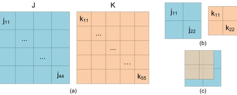
Figure 2.2 Spatial alignment problem: (a) Take some variablesJ, K at different spa-tial resolutions. (b) Try to define a transaction for the spaspa-tial point j11, requiring J and K be overlapped. (c)j11 overlaps k11, k12, k21, k22. . . . 11
Figure 2.3 Spatially-defined variables’ anomaly presence or absence is affixed to cli-mate index anomalies expanded to represent a global effect. . . 12
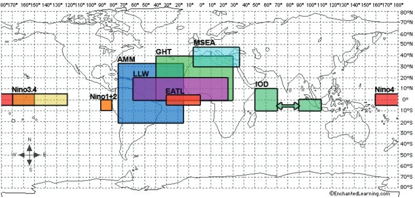
Figure 2.4 Climate indices can be distant, or many times partially co-located, com-plicating spatial alignment. . . 14
Figure 2.5 CHARM flowchart . . . 15
Figure 2.6 Data coupling for λi =EAT L8 and δj =N AO3. . . 18
Figure 2.7 Heterogeneous rule sets are generated for each coupling inciter. . . 20
Figure 2.8 Biclique mapping example . . . 24
Figure 2.9 Example bicliques for edges conserved across coupling inciters in Figure 2.8 24 Figure 2.10 Number of relationships found in network, averaged across coupling inciters . . . 31
Figure 2.11 Resulting combined network for coupling inciterEAT L8 . . . 33
Figure 2.12 Number of relationships found directly related to rainfall, averaged across coupling inciters . . . 34
Figure 2.13 Relationships directly associated with rainfall forλ=EAT L8 . . . 34
Figure 3.1 Illustrating a multi-phase physical system’s Gibbs free energy profile . . . 41
Figure 3.2 Methodology flowchart . . . 44
Figure 3.3 Leave-one-out (LOO) Cross Validation Results for North Atlantic Region TC Counts . . . 50
Figure 3.4 Features selected for East Sahel Rainfall Prediction use case . . . 54
Figure 4.1 CHARM-feature construction flowchart . . . 61
Figure 4.2 CHARM-constructed features retained per fold during LOOCV. . . 66
Chapter 1
Introduction
Numerous scientific fields are increasingly relying on data mining approaches to obtain mean-ingful information from large datasets that could be critical to the advent of new technologies
and processes. In recent years, climate science is shifting from solelyhypothesis-driven research
to the application of approaches that require a more dogmatic data mining implementation, already proving to be an effective tool to solve typical domain problems [24, 37, 118]. This
shift is similar to changes taking place in other domain sciences, like microbiology, where the
vision is that the rapid technological advances in data science will soon dominate hypothesis-driven research, given its ability to address inherently complex systems and provide insight
latent in already-existent data [88, 91]. The intent of applying thesedata-driven approaches to
such climate science implementations is to provide procedural and repeatable methodologies that provide physically-relevant results. In doing so, climate scientists obtain tools for modeling
system behavior that complement thehypothesis-driven methodologies they already employ in
a manner that can give consistent results with quantifiable accuracy, while also enabling the discovery of new hypotheses and phenomena within the data they already collect [88, 105].
Complex dynamic physical systems, such as those motivating this thesis, are inherently
complex. This complexity arises from the selective and nonlinear interconnections of functionally diverse components to produce coherent behavior. These systems often function in multiple
phases, described as having similar defining characteristics but whose feedbacks behave in
non-linear fashion. Within each phase, a system can be described non-linearly, but driven by minimization of Gibbs free energy [27], it undergoes transitions with strongly non-linear behavior that can
be treated within Landaus theory of phase transitions [57] (see Figure 3.1). The most simplistic
example includes the transition of a piece of ice from its frozen state through the liquid state to the vapor state upon being applied high temperature over time. Likewise, the steady state
The promising approach to providing mechanistic and predictive understanding of a system’s
dynamics and function aims to discover “hot spots” (informative features) that are responsible for (or specific to) a particular system’s state and to find (non-)linear relationships among those
features that closely approximate fundamental principles governing the complex behavior. This
approach essentially consists of the three major steps: (1) identification of phase transition points/intervals; (2) discovery of phase-specific “hot spots” (discriminative features) of the
system; and (3) inference of the relationships among those features that collectively define
the system’s (non-)linear response (e.g., cause-effect relationships). For example, the ENSO sea surface temperature anomaly index over the tropical Pacific (i.e., “hot spot”) captures
the fluctuation between the El Nio (warm) and La Nia (cool) oscillations (i.e., phases) that
cause extreme events (i.e., cause-effect relationship), such as floods and droughts in many regions of the world. The phase transition points of the target system can be defined—in a
supervised manner—by domain scientists based on the laws of physics. Otherwise, they should
be automatically predicted—in unsupervised fashion—from the real-world data using methods for phase detections, such as those described in §3.3.4.
Methods often employed by the aforementioned hypothesis-driven research activities have
not been found to be entirely robust in terms of accounting for a dynamic system’s characteris-tics. Many previous works in climate fields begin by selecting the correct data to utilize, given
the spatio-temporal nature of climate data, based on a priori knowledge of interrelated climate behaviors. This data is then extracted from the very many data sets collected by different
agencies and research institutions, with varying resolutions and collection windows, and more
importantly, of varying reliability. Given such inconsistencies, the domain sciences have moved to employ experiments utilizing more centralized methods of collecting and monitoring data,
making the data utilized more robust, but the selection of relevant data features still an ad hoc
process. Specifically, researchers in these fields often rely simple correlation metrics (i.e. Pearson or Spearman correlations) to determine if two particular climate variables are related, and use
such variables only if they meet a predetermined cutoff value [12, 53, 32]. Other works rely on
prior knowledge of relationships captured in literature to justify ad hoc feature selection and validate the results obtained, potentially ignoring patterns in other features that can influence
the models being generated [104].
This process of ad hoc or correlation-based selection does not necessarily mend with the inherent complexity of the climate system, as many climate processes are heavily affected by
anomalous behavior, and the timeframe of such anomalies can have a huge impact on final
climate outcomes. These temporal scope of these anomalies is very important, as the system can behave in a phase-based manner for which the characteristics can appear very similar but
the feedback itself is non-linear, but in possibly systematic temporal windows [27]. The key point
with the identification and prediction of the phases themselves. It is important to note that
studying relationships between spatio-temporal variables is rooted in obtaining in understanding of not only how pairs of variables are related, instead also observing how groups of variables
interrelate, as well as the particular temporal relationships between them. As aforementioned,
the complex dynamic system of climate can present relationships where the system feedback is in response to climate features that were anomalous months before. Hence, any methodology
that constrains the search space via feature selection or extraction has to account for possible
lags and ensure physical relevance for such lag times (i.e. no system feedback can be predicted using features occurring after the feedback’s time window).
However, these approaches are met with multiple challenges, a very latent one being the data
itself. The complexity of the climate system leads to very many climate factors being studied individually, at different spatio-temporal magnitudes and often in a three-dimensional space.
Another problem with this is the availability of historical data. The Extended Reconstructed Sea
Surface Temperature (ERSST) timeseries includes data starting in 1854, but many other climate datasets only include data from 1970 onward [102, 80, 101]. Further, the definition of a feature
in the climate context typically corresponds to a specific variable at a specific spatial location,
making there be many more available features than actual observational samples of such data, making this an underdetermined problem. Present works for hurricane and rainfall prediction
rely correlation-based feature selection strategies, coupled with linear regression techniques [12, 32, 53, 54, 55, 123] to predict system feedbacks. However, as aforementioned, this is not
necessarily advantageous when working with systems that can operate in multiple phases, such
as the complex dynamic climate system.
Another challenge is that many machine learning methodologies operate in exponential
time, so the magnitude of data available for the climate domain over-encumbers methodologies
unsuitable for handling such a high number of features being studied [107, 129]. Previous works on finding relationships of spatio-temporal datasets delve into finding events that co-occur at
distinct spatial locations. Approaches such as co-location pattern mining address spatial
re-lationship mining problems, taking a slice of spatial data and identifying rere-lationships based on the spatial proximity of events of interest [43]. However, in climate this is not necessarily a
feasible approach given it would prune correlated events occurring at large distances due to lack
of proximity, but these relationships, referred to as teleconnections, are of great informational value. These teleconnections may operate at great distances and still influence other driving
factors and overall system behavior [107]. Moreover, temporal aspects have not yet been
ex-tensively worked into co-location rule mining, and the methods for their evaluation are still limited.
We address these challenges by developing and applying three technologies to mine
1.1
Coupled Heterogeneous Association Rule Mining (CHARM)
Identifying the existence of co-occurring events in underlying data is a problem that has been
long addressed by Association Rule Mining (ARM) methods, typically under the application realm of transactional market-basket data [1]. Methods have also been developed for the
identifi-cation of sequential events in this data by means of mining sequential patterns and constructing
association rules from them [2]. Methodologies derived from these concepts have been applied to the climate domain with some success, limited by the scope of the data ascribed and the
organization of the data itself into structures that retain physical relevance in accordance to
the information desired to be extracted [19, 107]. The main problem in these approaches is the aforementioned varying resolutions of available climate datasets, which inhibits the
organiza-tion of data into proper transacorganiza-tional structures without the use of mathematically-constructed data values via interpolation or extrapolation [28]. The use of such mathematically-constructed
data would restrict the value of the information attained given the instability it introduces in
the data, making the identification of truly anomalous events vaguer. Other methods such as co-location mining [125] can be more suitable for such varying data resolutions, but have their
own detriments, specifically when applied to a climate context. Firstly, the methods for
find-ing relationships of anomalous event tend to rely on physical proximity, whereas in a climate context, important relationships can occur over very long distances and have a strong overall
effect on particular system and sub-system feedback behaviors. Furthermore, their applications
in a temporal context are limited, eliminating a glaring need of the climate community of understanding such relationships over time.
Given these factors, we leverage climate indices as an abstraction of complex behaviors in a
climate system [22, 36] and propose adata coupling structure that ensures all climate indices are considered to have some time-lagged relationship, regardless of their spatio-temporal proximity.
These relationships intend to capture how abundant one climate factor is in the presence of
another climate factor, and allow us to identify the anomalies of this abundance. We then use this information to mine the associations in these relationship anomalies. Doing this, we obtain
sequences of anomalies in the form of association rules that lead to a description of the events
that lead to a specific climate system feedback.
This approach also requires we have metrics to assess the significance of every rule generated,
as none of the traditional metrics have been found to be a “catch-all” for identifying significant
rules [107]. As such, we employ a Monte Carlo simulation to assess the possibility of finding any specific rule at random, and remove rules with low statistical significance from consideration.
Results indicate this methods is very effective at capturing known climate relationships and proposing new relationships to study. Results of the methodology are in line with climate
at a given time affects the overall climate system. Furthermore, study of the rules generated
allow for the attainment of more complex relationships in the underlying climate data that has been previously hypothesized but has not yet been fully understood.
1.2
Hierarchical Classification-Regression Ensemble for
Multi-Phase Non-Linear Dynamic System response Prediction
We address the problem of effective quantitative prediction of system feedbacks based on the
system’s present phase. As aforementioned, complex dynamic systems can behave differently in different phases, affected by the system’s behavior specific to that given phase. The main
challenge in this approach is having the ability to detect the system’s phase and employing an
effective methodology to account for possible outliers in the predictions, and as such generating predictions that are in tune with the system’s predicted phase, ideally increasing the accuracy
in predicting the overall system behavior. The first step in the process is to reduce the number
of features, which as aforementioned can be in the scale of thousands or hundreds of thou-sands, given the varying resolutions in the underlying data. A feature space of this very high
magnitude, given the aforementioned lack of observational samples, can lead to the “curse of
dimensionality” [8], possibly making many existing methods ineffective and inaccurate in their prediction capabilities.
As such, leverage the Forecaster classification model to iteratively select feature subsets
that discriminate between system feedback classes mapped to the physical system phases via a decision tree algorithm. This would provide an ensemble of selected features, while this ensemble
of classification models also provides information regarding the system’s phases as being in the
upper, lower or middle 33rdpercentiles [11]. Given this information, we leverage Least-Absolute-Deviation (LAD) regression to create an ensemble of regression models that capture linear
behaviors within individual system phases of each ensemble member. This method hypothesizes
that the accuracy of predicting system feedbacks is increased with prior knowledge of the system’s phase when the prediction is made, as similar feature conditions are considered in the
models pertaining to each individual phase. Doing so ensures the classification results tie in
precisely to the regression models, as the feature groupings identified by Forecaster are then used by the LAD regression models, to ensure that the regression models correspond to each
phase’s conditions.
This methodology is designed to work with the highly underdetermined problem, given the
ensembles it creates. However, considerations have to be made in order for the results to be
methods for regression ensemble model combination are not well-suited for LAD regression
models, so statistical methods must be employed.
Results indicate this method is very effective at addressing the phase-wise regression
prob-lem, improving model accuracy over previous works that solely employ correlation-based feature
selection and linear regression methodologies. Furthermore, study of the regression coefficients for each feature across different phases highlights that certain features are weighted differently
when built for different system phases, confirming the physical hypothesis.
1.3
CHARM-driven feature construction: Application to
cli-mate phase classification prediction
Given the information obtained with CHARM, we can identify key factors that interact in the complex dynamic system of climate along with those that affect the overall system response.
In order to further augment our knowledge of the climate system in its overall behaviors, we
see these newly found feature relationships as a means with which to ascertain how the system phases are affected by these relationships (e.g. negative anomaly phase of one climate factor
at a given time leading to a positive anomaly phase of another climate factor at a subsequent
time). The system behaviors themselves, related to one another, can tell us about the pathway that should lead to specific system response phases, so we propose using these relationships as
predictors in a classification model that can further elucidate information about climate system
interactions. This will allow us to contribute to overall system predictability given a small subset of measurable climate factors.
Again leveraging climate indices as an abstraction of complex behaviors in the climate
sys-tem [22, 36], we obtain a means with which to reduce dimensionality and further handle the underdetermined nature of the current climate data sets. As such, leveraging this abstraction
also provides a means to train classification models that capture behavioral relationships, and
as such can provide a means with which climate scientists can further gain knowledge of the system’s internal interactions. However, this can lead to models with low-order relationship
in-formation, lacking the structure to capture temporal relationships between features and instead
only assume relationships between individual climate factors and the system response.
As such, we propose applying the rules generated by executing CHARM, and leveraging
the knowledge of an internal relationship between climate factors, and the external relationship between these climate factors and the system response. As such, CHARM would in turn reduce
dimensionality of the raw climate index set, and provide new information by using coupled
(MNLR), given the data to be studied is already in multinomial nominal form, identified as
classes HIGH, LOW, and NORMAL. This would allow us to contrast the complex behaviors of the network against a simpler understanding based on raw climate indices. The novelty claim
for this approach in a research track is the usage of CHARM as a preprocessing technique in
Chapter 2
Coupled Heterogeneous Association
Rule Mining (CHARM):
Application toward Inference of
Modulatory Climate Relationships
2.1
Introduction
The climate system is inherently complex, due to the existence of non-linear interactions, or couplings, between its subsystems (e.g., the ocean and the atmosphere), global scale temperature
anomalies (e.g., El Ni˜no-Southern Oscillation), and other climate behaviors. Such a system
exhibitshierarchical modularityof its organization and function [39]: each constituent subsystem performs a similar function and does not act in isolation; instead, they interact or cross-talk.
The challenge is to discover the key subsystems and their cross-talk mechanisms; that is, the
positive and negative feedbacks that collectively modulate the dynamic behavior of the system through a sophisticated network of modulatory pathways that ultimately define the system’s
functional response.
For example, the rainfall anomaly in the Sahel region of western Africa, which is the fo-cus of this study, represents a functional response of the climate system. Rainfall in the Sahel
is dependent on global Sea Surface Temperature (SST) patterns, as well as on local climate
variability. There is a multitude of complex associations between various subsystems that drive the Sahel’s climate response mechanisms. Some of these associations have been discovered
throughout more than two decades of hypothesis-driven and/or first-principles based research.
Mediter-Figure 2.1: Complex relationships between climate indices and Sahelian rainfall, with some direct and indirect relationships well defined in literature (light arrows) and others not fully understood (dark arrows)
ranean Sea (MSEA) and the warm phase of the Atlantic El Ni˜no-Southern Oscillation (EATL)
being associated with rainfall deficiencies over the Sahel [94, 48]. Figure 2.1 illustrates a climate
modulatory network, which is a collection of modulatory pathways, with some mechanisms driving rainfall in the Sahel known to be directly/indirectly associated, and some not fully
understood. Comprehending these mechanisms is particularly important due to the influence
of rainfall variability in the region on the occurrence of meningococcal meningitis. When the Sahel is dry (i.e., negative rainfall anomaly), the regional conditions favor meningitis epidemics
and vaccination should be planned to prevent the spread of the disease [109].
For mechanistic understanding of functional responses such as African Sahel rainfall, we posit that a data-driven approach may facilitate the discovery of key factors that might
cross-talk by identifying candidate modulatory pathways and/or suggesting new factors and relation-ships with the proper characterization of their inductive or suppressive roles. The goal of our
approach is to elucidate the putative modulatory pathways that suggest cross-talking
mecha-nisms controlling a system’s functional response. More specifically, given the key climate drivers and their modulatory directions on the response, we must infer (a) the putative pathways of
modulatory signs (e.g., induction vs. suppression, such as a positive anomaly sign of EATL,
EATLHIGH being related to the negative anomaly sign of Sahel rainfall, RainfallLOW) that
collectively define the network of modulatory pathways for the response. Furthermore, given
that there is a variety of methodologies that can be used to find such modulatory relationships,
we must provide a consensus result that accounts for all evidence of a given relationship. To the best of our knowledge, this is a novel proposition in the field of knowledge discovery in
the physical science domain, in general, and climate extremes (e.g., droughts), in particular.
Moreover, this data-driven approach could contribute, in the long run, to the identification and characterization of more comprehensive and predictive models of the physical phenomenon
under study.
2.2
Challenges and Contributions
Given the intent of finding modulatory associations between distinct climate factors across
dis-tinct spatial locations, we introduceCoupledHeterogeneousAssociationRuleMining (CHARM). CHARM is an extension of association rule mining (ARM) that enables the discovery of
climatologically-relevant modulatory pathways from spatio-temporal climate data. CHARM
relies on another concept we introduce herein,data coupling of climate indices, which serves a mechanism of modeling the strength and the sign of the anomalous effect of one climate system’s
component (i.e., climate index) relative to another. We then use this concept to predictively
mine higher-order (possibly non-linear) couplings between these subsystems’ anomalous tem-poral phases with respect to their overall modulatory effect on the system’s functional response
(e.g., Sahel rainfall anomalies). This translates to finding climate phenomena which are
inher-ently causal to rainfall over the African Sahel region.
Each climate phenomena (e.g. Sea Surface Temperature, Sea Level Pressure, etc.) is of
dimension t×k, wheret and k represent temporal and spatial dimensions, respectively. Thet
dimension is often of varying time scales, as data is collected at varying times throughout the year. However, the k dimension of each phenomena is not necessarily of the same magnitude, making this a key design factor for data pre-processing must account for this. In the context
of climate science, year-to-year trends are of particular interest, but month-to-month behaviors are important in terms of predictability. This leads data organization to bef×y, consisting of
f features, where f represents a specific climatological phenomena at a given spatial location and minor time unit (i.e. month), andy being the major time unit (i.e. year), which introduces additional complexity, as discussed in§2.4.4.
To address these issues, we focus on sequential relationships presented as rules that capture the behavior of the overall climate system. The proposeddata couplingenables the
Figure 2.2: Spatial alignment problem: (a) Take some variablesJ, K at different spatial resolu-tions. (b) Try to define a transaction for the spatial pointj11, requiringJ andK be overlapped. (c)j11 overlapsk11, k12, k21, k22.
discovery of modulatory pathways that confirm known (or reveal new) control mechanisms that
drive the Sahel climate anomaly. This adaptation requires overcoming a number of technical
challenges herefore briefly articulated.
2.2.1 Spatio-Temporal Misalignment of Key Factors
As illustrated in Figures 2.1 and 2.4, key climate drivers, represented here as climate indices,
can be spatially displaced or partially overlapping, while also active at different temporal phases
in the modulatory network of the Sahel climate anomaly. To the best of our knowledge, present ARM methodologies are not well-equipped for handling such diversity in the spatio-temporal
alignment of its system’s features. Firstly, the transactional nature of the ARM methods requires
that identifiers of transactions, or rows in the transaction matrix, describe each spatial grid point (i.e., latitude, longitude, and/or altitude) at a given point in time (i.e., month and year).
Furthermore, present methods enforce the alignment of all features, or columns, with respect
to their corresponding transaction IDs.
Some climate variables from observations or simulations (e.g., SST) are defined only over
the ocean; yet others (e.g., rainfall) are defined over land. Hence, considering both features as columns in a transactional matrix is impossible, given that they have no common grid points.
Even if they share some spatial region, they are often still misaligned due to variation of their
grid resolutions. While mathematical methods (e.g., interpolation or extrapolation) exist to fa-cilitate data alignment, they introduce uncertainty and instability, affecting the interpretability
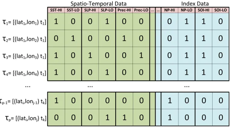
Figure 2.3: Spatially-defined variables’ anomaly presence or absence is affixed to climate index anomalies expanded to represent a global effect.
and the aforementioned mathematical operations must be performed again.
An ARM-based approach for the discovery of relationships among climate variables was
proposed by [107]. This approach studies only spatially-aligned datasets, and affixes climate
indices alongside them. However, due to its inherently grid-based nature, this approach assigns each climate index’s locally observed anomalies to all grid points. That is, it assumes that the
anomaly equally affects the entire globe. While such an assumption may hold for some climate drivers, it can increase the number of false positives due to its inherent amplification bias. For
example, in the representative case shown in Figure 2.3, the high anomaly of the SOP index
(SOI-HI) and the low anomaly of the NP index (NP-LOW) would be present in every itemset for time tk, which complicates understanding the information gained from any resulting rules
that includes them.
Likewise, co-location pattern mining approaches address the spatial misalignment problem, taking a slice of spatial data and identifying relationships based on the spatial proximity of
events of interest, using a transactionless setup [43]. In climate, this is not necessarily a feasible
approach given it would prune correlated events occurring at large distances due to lack of proximity, but these relationships, referred to as teleconnections, are of great informational
value. Theseteleconnections may operate at great distances (see Figure 2.4) and still influence
are still limited.
In this chapter, we leverage climate indices as an appropriate abstraction for individual climate system behaviors and presentdata coupling as a methodology to describe relationships
between climate factors possibly occurring on different parts of the globe and at different times,
making it suitable for mining complex spatio-temporally misaligned associations between key climate drivers. In addition, this makes ARM algorithms computationally tractable due to a
significant reduction of the number of transaction IDs to a few thousands from hundreds of
millions, considering typical monthly data over 100 years and 0.5◦ ×0.5◦ spatial resolution. Data coupling is described in more detail in §2.4.2.
2.2.2 Lack of High-order Associations
Present association analysis techniques treat system components (e.g., climate indices) as atomic instances of presence or absence [107] and, to some degree, ignore the intertwined coupling
be-tween them. For example, entropy is defined as the ratio of the heat transferred bebe-tween the
system and its surrounding to a temperature at which this transfer occurred. The significance of such a ratio comes from the fact that energy added to the system in a form of heat at a lower
temperature produces much larger change in its configurational state than the same amount
added at a higher temperature. Another example of contextual coupling of the system’s factors via ratios is in resonances. Namely, in a forced oscillator, the external excitation frequency
ap-proaching the natural oscillator frequency creates a dramatic increase in oscillation amplitude,
proportional to the ratio of the external force to a squared difference between the excitation fre-quency and natural frefre-quency of the system. Finally, in the climate domain, the North Atlantic
Oscillation (NAO) index is a coupling of a temperature gradient with a pressure gradient.
Capturing higher-order couplings that include multiple system components, such as the ones above or depicted in Figure 2.1, would require an ARM algorithm run for a large number of
items in the resulting itemsets. Since the maximum size of the itemset contributes exponentially
to the computational complexity (see§2.4.4), when performed over the transaction matrix with millions of IDs, such algorithms require impractical computational time.
In the temporal space, sequential ARM intends to work with lag and lead times for the same
feature [2, 44], but our intent is to pursue the analysis ofcomplex relationships in data, which would include different variables over different times and different spatial regions of influence.
To address these issues, we propose to quantify the putative coupling between various climate
indices by employing the concept ofrelative abundance, allowing us to measure the strength of the anomalous event due to the co-occurence of one climate factor with another climate factor
Figure 2.4: Climate indices can be distant, or many times partially co-located, complicating spatial alignment.
details of this methodology are discussed in§2.4.2.
2.2.3 Rule Significance
Traditional ARM requires a preset support and/or confidence cutoff to prune the search space,
and there is no set standard as to selecting said cutoff, and any threshhold tweak would impose
recomputation. Different metrics exist to provide different amounts of information of the gen-erated rules given statistical implications. More importantly, even rules conforming to the set
thresholds, or having seemingly favorable metrics cannot be blindly confirmed as statistically
significant, as there is no guarantee that data at random could not generate the same set of rules, so additional significance analysis is required. We discuss a strategy for accomplishing
this in§2.4.3.
2.3
Related Work
The ever-evolving field of knowledge discovery is often entrenched in works related to association
rules. The numerous spatial relationships along with the continuous nature of spatial events hinders association rule mining applications from discovering co-location patterns [43]. This
hindrance is partly caused by the terminal nature of association rules – reusing them could
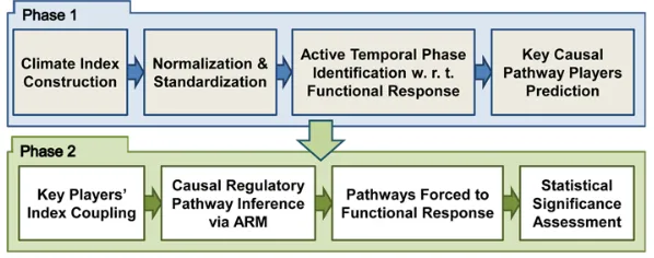
Figure 2.5: CHARM flowchart
such patterns often employ clustering algorithms; thus papers in this area are often tested for performance speed instead of field applicability [43, 124]. Due to the continuous nature of spatial
events and, oftentimes numerous spatial relationships, discovering co-location patterns can be
difficult.
Real world applications of finding such associations by measuring their significance based on
the underlying field sciences is explored in [107]. However, as mentioned throughout the chapter,
while the method in [107] designs their methodology to utilize grid cells for spatio-temporal data, we utilize a combination of climate index references and time as transaction identifiers.
This addresses the issue of generating too many associations among events abstracted from the
climate indices identified in this chapter.
2.4
Method
Figure 2.5 shows an overview of our methodology. We first prepare the input data through a synergy of data preprocessing and pruning methods. We then employ the Lasso multivariate
regression [111] as described in [84] to infer the causal relationships among the variables of
in-terest and identify the key factors in the network of modulatory pathways. Given the results of this (captured mostly in Phase 1 of Figure 2.5), we calculate asymmetric ratios using the
iden-tified key factors to create data couplings of climate indices, and employ percentile thresholds
for detecting HIGH and LOW anomalies with respect to the desired response (i.e., rainfall), setting the framework for complex relationships. We then heterogeneously infer modulatory
pathways via higher-order association rule mining, in the form of sequential association rules
2.4.1 Identification of key factors in the climate causal network
Previous works present a method toward a data-driven, semi-automatic inference of
phenomeno-logical model explaining the eastern Sahel rainfall variability [84]. It identifies the intrinsic
causal relationships among the local and global climate variables and the Sahel rainfall using the Lasso multivariate regression. It also proposes methods for pruning the search space,
signifi-cance estimation and impact analysis that provide quantifiable metrics—in terms of predictors’
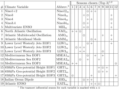
contributions to the rainfall variability and their probability of detections (PODs). Hence, we employ the methodology suggested in [84] to identify prominent seasons in the data, highlighted
in Table 2.1 [84]. The approach in [84] is then validated by the fact that the results are
con-sistent with many of the well-known causal relationships from prior climatological knowledge [10, 67, 106]. The results in [84] complement the existing physical models and help climate
scientists derive a stronger physical rationale for the eastern Sahel rainfall variability.
ARM is an increasing area of interest for domain sciences, because of the growing need
to mine data to identify the co-occurrence of important events [87, 107]. ARM, unlike other
methodologies for inference of phenomenological models, takes into account the latent but vital signals embedded in the intermediary pathways associated with the system’s functional
response. We expect that this segment of our study, combined with [84]’s work, could contribute
to isolating preferentially plausible and inherent pathways by which the methodology may describe sub-region’s climate variability, given some predefined, climatic antecedents.
2.4.2 Coupling of Climate Indices
Due to the complexity of the climate system, building comprehensive models over climate data
is not trivial. Climate data presents a challenge to traditional ARM techniques in terms of data dimensionality and structure, given that it can be captured at various resolutions and time
spaces, with varying magnitudes and representations.
The key drivers of a climate system are spatially distributed and active at different temporal phases in the modulatory network of the system’s functional response. State-of-the-art mining
methodologies are not well-equipped to handle such diversity of spatio-temporal misalignments between the system’s features. For example, due to the transactional nature of the ARM
meth-ods, each spatial grid point (specified by latitude, longitude, and/or altitude) at a given point
in time (e.g., month and year) defines a transaction ID, or a row in the transaction matrix. This requires that all features be aligned with respect to their transaction IDs, complicating
the use of multi-resolution, multi-variate, spatio-temporal climate data by these methods. For
this reason, we leverage climate indices, known to be a valid abstraction of the underlying sub-system’s zonal climate behavior [36], thus significantly reducing the number of features needed
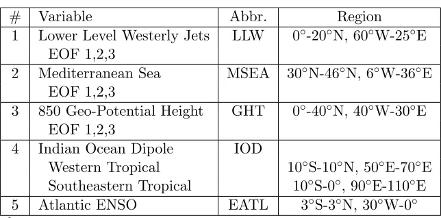
Table 2.1: Average prominent season selections for climate variables over 1000 iterations
Seasons chosen (Top 3)1,2
# Climate Variable Abbrev.3 1 2 3 4 5 6 7 8 9 10 11 12
1 Nino1+2 Nino12m ⊕ + +
2 Nino3 Nino3m + ⊕ +
3 Nino4 Nino4m + + ⊕
4 Nino3.4 Nino34m ⊕ + +
5 Multivariate ENSO MEIm + ⊕ +
6 North Atlantic Oscillation NAOm + + ⊕
7 Atlantic Multidecadal Oscillation AMOm ⊕ + +
8 Atlantic Meridional Mode AMMm ⊕ + +
9 Lower Level Westerly Jets EOF1 LLW1m ⊕ + +
10 Lower Level Westerly Jets EOF2 LLW2m ⊕ + +
11 Lower Level Westerly Jets EOF3 LLW3m + + ⊕
12 Mediterranean Sea EOF1 MSEA1m ⊕ + +
13 Mediterranean Sea EOF2 MSEA2m ⊕ + +
14 Mediterranean Sea EOF3 MSEA3m + + ⊕
15 850hPa Geo-potential Height EOF1 GHT1m + ⊕ +
16 850hPa Geo-potential Height EOF2 GHT2m ⊕ + +
17 850hPa Geo-potential Height EOF3 GHT3m ⊕ + +
18 Indian Ocean Dipole IODm ⊕ + +
19 Atlantic ENSO EATLm + + ⊕
1
The topmost influential season for each variable is marked with a⊕ 2
1 = Jan-Feb-Mar, 2 = Feb-Mar-Apr,. . .,12 = Dec-Jan-Feb
3
Subscriptmrepresents chosen season (i.e. NAO3: Season 3 chosen for NAO)
in different parts of the globe (see Figure 2.4).
Climate scientists often study climate factors in a coupled manner and relate certain vari-ables to others. Traditional lagged climate techniques employed for coupled pattern analysis
include singular value decomposition, grid point correlations, among others [86]. For example,
Principal Component Analysis (PCA) has been used to determine the relationship between Indian Ocean Dipole and East African rainfall [97, 66]. Hence, we adopt a similar approach
by coupling climate indices. We take a quotient of these relationships before identifying any
anomaly, to capture the anomaly in the relationships between these variables.
For each climate index λ to be used as a coupling listener, we iterate through all other climate indices δ as coupling inciters, and calculate their ratio, δ/λ, as a data coupling that intends to capture the behaviors of the logical sentence “how abundant isδ given the presence ofλ?” An issue in calculating these ratios is the potential emergence of large values due to the denominator possibly being orders of magnitude smaller than the numerator. To handle this,
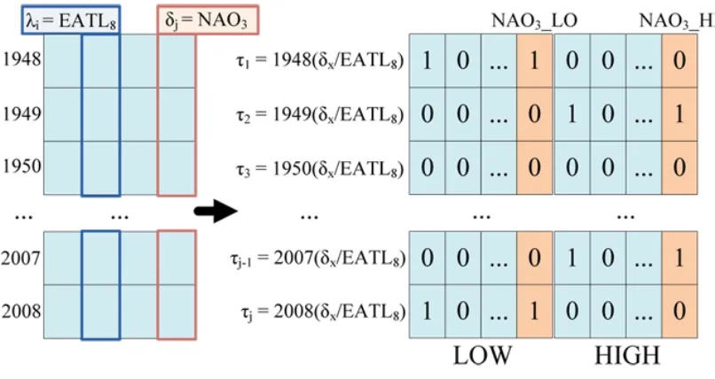
Figure 2.6: Data coupling forλi=EAT L8 and δj =N AO3.
to avoid wide-ranging quotients that could affect the abstraction of anomalous events (§2.4.2). We note that each tuple (row in the database) now represents a specific coupling inciter λ
and time, while each column represents a particular coupling listener δ, and each cell contains the relevant data coupling value. For ARM, this data must be binned, after which the resul-tant dataset cells indicate the presence or absence of anomalies for each previously calculated
coupling, described further in §2.4.2.
This process increases the size of the transaction matrix considerably, as we calculate each
possible combination of δ ∈ Λ and λ ∈ Λ, so the number of resulting tuples also increases based on the number of variables being used (represented as |Λ|), the number of months in a year, and the number of years in question. For example, given |Λ| distinct variables captured
using ρ= 12 phases acrossy ∈Nyears, data initially with dimensions [y×(12· |Λ|)] grows to [(12· |Λ| ·y)×(12· |Λ|)] . We address this significant data increase in Section 2.4.1, by reducing
ρ to the three temporal prominent phases (ρ= 3).
Identifying Anomalous Events
Following the norms established by NOAA1, we identify anomalies as any set of values below
the 33.33rdpercentile or above the 66.67thpercentile for any given variable. Given that the data was normalized before calculating ratios, we identify the anomalies using the aforementioned
norm, based on the phase-wise groupings. We take each tuple corresponding to each unique
combination of δ and λ, and identifyhigh anomalies as being those ratios in the upper 66.67th percentile, and low anomalies as being ratios in the lower 33.33rd percentile.
Since we are trying to identify the presence or absence of anomalous events, we divide each
column into two separate high and low cases, and assign a binary 1 when either anomaly occurs, and a 0 otherwise. This results in a very sparse matrix, as no particular year can fit in both
high and low categories, and it is likely the majority of years have most variables falling into a
non-anomalous category.
Figure 2.6 represents a particular (i, j)th iteration. In this example, for the coupling of
λi =EAT L8 and δj =N AO3, we identify high and low anomalies and assign transaction IDs that indicate that the cells pertain to the coupling of that year’s data for the listener (shown in the column header) against the stated inciter. This transaction ID shows that each row in
the matrix consists of the anomaly of the ratios calculated over each possible coupling δx/λi,
wherex indicates that all values in this row were divided by the sameλi.
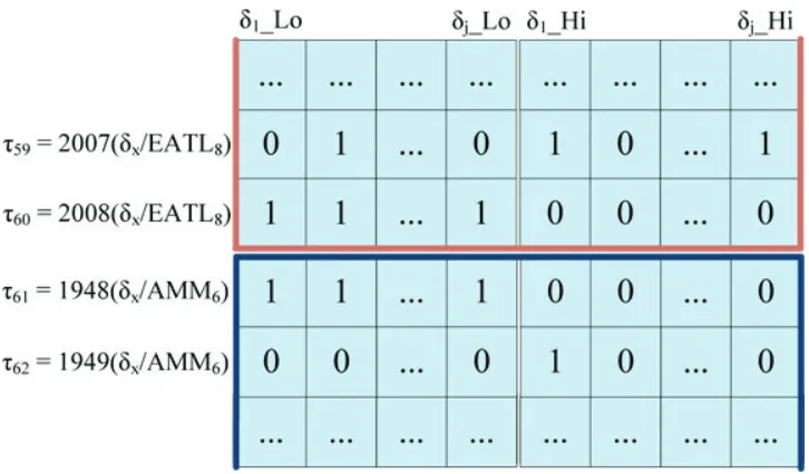
Coupling heterogeneity
Given the data couplings are being generated over varying coupling inciters, the methodology
creates a large set of transactions, covering each year studied for each particular possible
cou-pling inciter. Given it would be difficult to interpret rules that only have sufficient support because they are present over multiple inciters, we ensure rule generation is not performed
het-erogeneously, separating sets pertaining to different coupling inciters, as shown in Figure 2.7.
To this purpose, we divide the dataset into smaller subsets, such that we mine rules generated for each coupling inciter independently, allowing us to determine the presence of some
prefer-ential bias towards a particular coupling inciter. As such, this preserves information relating to
each data coupling individually, and can provide additional information from knowing which particular coupling inciters seem to affect coupling listeners to a point where the rules found
are interesting to domain scientists. We note that separating the data in this manner makes the
implementation similar to the per-customer groupings of AprioriAll [2], intentionally obviating cross-customer mining as it may be misleading in terms of how the indices are coupled.
2.4.3 Pathway significance assessment
As mentioned before, rule interestingness in ARM is estimated using metrics that quantify the importance of each rule. Selecting which metric to use depends on the information to
be obtained [107]. Support and confidence are commonly used to measure rule quality, and
Figure 2.7: Heterogeneous rule sets are generated for each coupling inciter.
off rules deemed “uninteresting”, which reduces the accuracy in retention of significant rules. Hence, we first prune based on bare-minimum thresholds for support and confidence (the rule
appearing in a single transaction), and if any given rule needs to be further analyzed (based
on domain knowledge or otherwise), we perform a Monte Carlo simulation to test against the null hypothesis of observing the rule at random. Thus, we define a rule to be significant and
interesting if it meets the following criteria: p-value ≤0.01, support≥6%, and conf idence≥
70%.
This criteria constrains the search space, and trims the result space, pruning unimportant
rules. Once a set ofpossiblyinteresting rules is identified, the computationally more demanding,
but embarrasingly parallel, statistical significance test is applied to further prune insignificant rules. On average, this removed 20-30% of the generated rules from the result set.
2.4.4 Computational complexity
Association Rule Mining is anNP-complete problem that, when setting a bound on the trans-action length, finding all frequent itemsets becomes linear with complexityO(r·n·2l), where
n is the transaction count,l is the maximum itemset length, and r is the number of maximal frequent itemsets [129]. Rules are generated such that a user-specified minimum confidence
minconf and/or a minimum support minsup is satisfied, and as such, for a given itemset of lengthk, there are 2k−2 potentially confident rules, and the complexity of this step becomes
itemset [107, 129].
In this paper, we leverage theApriorialgorithm to mine the desired rules [87]. The algorithm ensures only maximal frequent itemsets are considered, and is well regarded in ARM approaches
[1]. Furthermore, CHARM explores sequential ARM, which allows us to see if events transpiring
in different temporal instances are related within themselves [44].
Also, as mentioned in §2.4.2, each coupling inciter is studied independently in order to ensure data couplings are studied heterogeneously. This design also allows the methodology to
function in steps of smaller executions instead of a single, considerably longer execution. Given this division into smaller subproblems, the problem becomes embarrasingly parallel and can be
divided into parallelized tasks to help with execution times. Studying the combination of all
possible denominators is a topic for future work, and an implementation that considers these as appendable within transactional years is discussed in Chapter 4.
2.4.5 Obtaining additional relationship evidence
In this chapter, we also explore leveraging additional methods as a means with which to obtain additional evidence of the presence of a given relationship in the underlying climate data.
CoupledHeterogeneous AssociationRule Mining (CHARM) allowed us to minehigher-order
couplings of climate relationships and to capture the anomaly phases with which each climate factor is related to each other (e.g., a negative anomaly of LLW may be related to a positive
anomaly of EATL, and the presence of both factors may be associated with a negative Sahel
rainfall anomaly) [29]. Such relationships are not typically captured from modulatory inference frameworks, let alone traditional association rule mining (ARM) methodologies.
However, knowledge of relationships found by other methodologies can highlight how well
CHARM complements the information gained by leveraging it in conjunction with them, as well as highlight key differences in its ability to find relationships that are well-known from climate
literature. Hence, we extend CHARM by incorporating other existing methodologies, namely
Lasso multivariate regression [111] (§2.4.5) and Dynamic Bayesian Networks [72] (§2.4.5), as complementary approaches to increase the confidence of the inferred modulatory relationships.
Moreover, in order to obtain a consensus as to which of the relationships identified have the
most evidence of being present, we treat the results of each methodology as individual pieces of evidence in an information fusion approach, and combine them into a unified, coherent
result. This unified result can provide us a means with which to increase the confidence of the
relationships identified throughout the different methodologies. This should allow us to contrast the methodologies by studying how each of their results differ, and to correlate these results
scientists for further study.
Lasso Multivariate Regression
Least absolute shrinkage and selection operator (Lasso) multivariate regression is an approach
pioneered by [111] that takes a set of inputs and an outcome measurement and fits a linear model, seeking to shrink the regression and sparsify the predictor feature space. This is achieved
by constraining the L1 norm of the β parameter vector B ={β1, β2, . . . , βn}, calculated as in
Eq. 2.1, such that it is no greater than a given s value to be minimized [111].
L1norm=|B|1 =
n
X
r=1
|βr| (2.1)
In the context of this chapter, this process highlights the prominent phases of the features
(§2.4.1). It derives the temporal phases of predictors lagged behind a response of interest, gen-erating predictor coefficients indicating the magnitude and type of the modulatory relationships
with said response [84].
Recent work on inference of modulatory relationships based on Lasso multivariate regression of temporal and spatio-temporal data includes means to improve upon the Lasso methodology.
We apply the method proposed by [84], given that it incorporates prominent phase detection
and significance assessment. [84] presents an approach toward a data-driven, semi-automatic inference of phenomenological physical models based on the Lasso multivariate regression model
and quantifies the influence of key “players” on the response of interest (e.g., Sahel rainfall
anomaly) through use of the Expected Causality Impact (ECI) score. The work presented in [84] also proposes methods for search space pruning, significance estimation and impact analysis
that provide quantifiable metrics in terms of predictors’ contributions to the rainfall variability
and their probability of detections (PODs).
Dynamic Bayesian Networks
DBNs expand upon Hidden Markov Models (HMMs) and Kalman Filter Models (KFMs),
in-dexing instances of arbitrary variables. DBNs are represented as a structure similar to that of
Bayesian Networks with the added benefit of incorporating the temporal space [15, 72]. DBNs are a very popular means with which to mine and represent modulatory relationships in data,
given that the conditional probability distribution of each node can be estimated independently
[23, 72]. The model’s dynamicity is obtained by combining a traditional Bayesian network with a temporal Bayesian network that allows for capturing behaviors of the Bayesian network over
the temporal space, and is not to be confused with the idea that the model changes over time
2.4.6 Construction of Modulatory Networks
Each of the aforementioned methodologies presents results in a different manner, affecting the
interpretability of the information they provide. Hence, the resulting relationships between
climate factors should be structured such that all possible modulatory pathways are captured in a comparable context, while preserving the information given by each method.
The results provided by DBN capture a network of relationships between climate factors as
a directed, acyclic graph (DAG). Such graph includes a set of vertices and directed edges, which in the context of this study represent the climate factors and the relationships between factors,
respectively. This structure provides an intuitive visualization of the behaviors in the system,
as each edge represents the existence of a relationship between the climate factors it connects. Therefore, we adapt the results provided by CHARM to a similar structure, by building a
network where the edges represent each possible combination of high/low anomalies, directed from antecedent to consequent.
However, given that CHARM uses coupled climate indices, we must ensure the the networks
generated for the three methods can be equally interpreted. Hence, each Lasso and DBN exper-iment will also use such coupled data and will also be executed heterogeneously, as described in
§2.4.2. This allows us to directly use the results provided by DBN, given that it already adheres to the proper network structure. As for the results from the Lasso experiments, we generate the network of modulatory pathways by drawing a directed edge from vertexA toB when aβ
coefficient was found for an execution whereBwas the response andAwas a predictand. Given the temporal window constraints set upon this problem, we can follow the graph backwards from our desired response to study all relationships, both direct and indirect.
2.4.7 Modulatory network motifs across coupling inciters
The network structure obtained by employing these methodologies allows us to characterize the
relationships between coupling listeners in terms of direct and indirect modulatory relationships with the Sahel rainfall system response. Furthermore, given the potentially distinct edge
struc-tures between networks with similar vertex strucstruc-tures, we can leverage this organization to further study the network motifs present across multiple coupling inciters.
The motifs present across the different coupling inciters can be identified by performing
comparative analysis of the networks associated with the different inciters. Here we model the motifs as connected components conserved across the different subset of networks. The brute
force method of identifying the motifs from each network and then checking its presence or
absence in other networks becomes a computationally intensive and inefficient. Thus, we chose to combine these networks into a single network and mine the combined network for the network
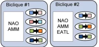
Figure 2.8: Biclique mapping example
Figure 2.9: Example bicliques for edges conserved across coupling inciters in Figure 2.8
present across different subsets of inciter networks. The second step parses each conserved edge
set to identify the connected components.
For the first step, we create a bipartite network B = (P1, P2, E), whereP1 and P2 are the two disjoint vertex sets ofB, andE represents the all edges between vertices belonging to P1 and P2.Each vertex in setP1 represents an coupling inciter and each vertex inP2 represents a temporally-directed edge between a pair of coupling listeners. An edge (u, v) is placed between vertex u ∈ P1 and v ∈ P2, if the temporally directed edges between pair of coupling listeners represented by v is found in the network associated with the coupling inciter represented by u
(see Figure 2.8). This network is mined for maximal bicliques to identify edge sets conserved
across different subsets of inciter networks. In the second step these, edges set associated with each biclique is processed to identify the connected components. These connected components
become the network motifs conserved across that particular subset of inciter networks (see
Figure 2.9).
2.4.8 Consensus Modulatory Network Inference via Information Fusion
To infer a consensus modulatory network for a functional system response, we must combine the
modulatory networks inferred by CHARM, Lasso multivariate regression, and DBN into a single