Electromagnetic fields in coupled cavities.

University of Windsor University of Windsor

Scholarship at UWindsor

Scholarship at UWindsor

Electronic Theses and Dissertations Theses, Dissertations, and Major Papers

8-13-1965

Electromagnetic fields in coupled cavities.

Electromagnetic fields in coupled cavities.

Bing Yiu Tam University of Windsor

Follow this and additional works at: https://scholar.uwindsor.ca/etd

Recommended Citation Recommended Citation

Tam, Bing Yiu, "Electromagnetic fields in coupled cavities." (1965). Electronic Theses and Dissertations. 6405.

https://scholar.uwindsor.ca/etd/6405

ELECTROMAGNETIC FIELDS IN COUPLED CAVITIES

BY

BING YIU TAM

A Thesis

Submitted to the Faculty of Graduate Studies through

the Department of Electrical Engineering in Partial

Fulfillment of t h e 'Requirements for the Degree

of Master of Applied Science at the

'University of Windsor

Windsor,' Ontario

UMI Number: EC52586

INFORMATION TO USERS

The quality o f this reproduction is dependent upon the quality o f the copy

subm itted. Broken or indistinct print, colored or poor quality illustrations and

photographs, print bleed-through, substandard m argins, and im proper

alignm ent can adversely affect reproduction.

In the unlikely event that the author did not send a com plete m anuscript

and there are missing pages, these will be noted. Also, if unauthorized

copyright m aterial had to be removed, a note will indicate the deletion.

®

UMI

C opyright 2008 by ProQ uest LLC.

All rights reserved. This m icroform edition is protected against

unauthorized copying under Title 17, United States Code.

ProQ uest LLC

Approved by:

\A\C. /&.L'ls£u2.

ABSTRACT

Two cavities resonating at about the same

frequency are coupled with each other through a small

iris closed hy a thin partition. The radius of this

iris is assumed to be small compared with the wave­

length. If one cavity is excited, fictitious surface

magnetic charge and a fictitious surface magnetic

current density are formed in the iris. The distribut­

ion of these magnetic charge and current densities

constitutes a boundary condition for the calculation^

of the electromagnetic fields in the cavities. This

solution is in terms of certain orthogonal functions

of the separate cavities.

hCIRTOWIEDGEkEK'TS

The author gratefully acknowledges the able

direction of Dr. S. N. Kalra, under whose suggestion

these' studies were undertaken. In particular the

author wishes to express his thanks to Dr. P. H o l u j ,

Dr. E. P. Hsu and Dr. H.H. Hwang for their excellent

advise and encouragement. Financial assistance was

provided by the National Research Council of Canada.

Page

ABSTRACT ... ii

A C Of 0WLEDGEKEN T S ... iii

1. INTRODUCTION ... .... ... 1

2. .THE COMPLETE EXPANSION OP ELECTROMAGNETIC

FIELDS IN CAVITY RESONATORS ... 4

3. ASSUMPTIONS AND BOUNDARY CONDITIONS ... 11

4. SURFACE MAGNETIC CHARGE L CURRENT

DISTRIBUTIONS ... 1?

5. GENERAL-FIELD SOLUTION ... 24

6. EXAMPLE ... ■... 32

APPENDIX

A. Vector and Scalar Functions ... 41

B. Orthogonality ... 47/

BIBLIOGRAPHY ... " ' 54

1 . INTRODUCTION

An electromagnetic field vector function, as

defined by Helmhotz, can be represented by the sura of an

irrotational function and a.solenoidal function. This

concept was first applied to the theory of cavity reso­

nators by Slater [ 1] . However, he considered that

on-iy the electric field in the cavity consists of both

irrotational as well as 'solenoidal fields; that the

magnetic field, on the other hand, has no irrotational

part. later, .Teichmann and Y/igner [2] pointed out that ■

a complete expansion of electromagnetic field should

include the irrotational magnetic field which w a s found',

to be inversely proportional to its frequency Basing

on this suggestion, Kurokawa [3] gave a proof that for a

complete expansion of electromagnetic field it is neces­

sary to* add the irrotational component in the magnetic

field. He asserted that if the irrotational component

was neglected, there would be no' magnetic field through

the opening of the cavity at all when the cavity is

coupled.to a waveguide through an iris.

Cavity coupling systems have long been used and

2

studied by physicists and engineers. Either, in experi­

mental or in theoretical analysis, they are generally

considered as equivalent admittance or impedance circuit

representation in form of parallel or series resonant

circuits or both [4] • The coupling device is repre­

sented by an equivalent capacitive reactance if electri­

cally coupled; by an equivalent inductive reactance if

magnetically coupled [5 ] . This approach has little or

no contribution to the analysis of the fields in the

coupling systems. Up to present time, not much effort

has been made on the field analysis as yet.

For most common practice, the cavities are

coupled through apertures. The degree of coupling is

depending on the sise and shape of 'the aperture. If the

aperture is large, there are many difficulties in dealing

with the field analysis of cavity-coupling problem:

large disturbance due to the presence of the aperture,;

strong interaction due to the infinite number of reflec­

tions of fields.between cavities; and the unknown field

distributions in the region of the aperture. On the

other hand, if the aperture is small, all these field

perturbations may.be negligible and an approximation

method may be applied in solving this problea. In this

thesis, the author makes an attempt- to work out the

5

the theory of cavity resonators and the Bethe's method

of the field diffraction by small holes [6"] . An

example is also given to illustrate the application of

2. SHE COMP LEI'2 EXPANSION 01' ELECTROMAGNETIC FIELDS

IN CAVITY RESOLATORS

Resonance phenomena may occur in a number of

types of structures which are used in microwave system.

Any volume completely enclosed by a conductor is usually

called a cavity resonator. In distinction with a lumped

constant resonant circuit, a cavity resonator can reso­

nate at an infinite number of discrete frequencies. The

electromagnetic fields in a cavity resonator can be re­

presented by the sum of modes of certain frequencies of

oscillation which are' the characteristics of the eigen­

values of the wave equation with suitable boundary con­

ditions. Both for electric field and magnetic field at

an interior point in the cavity resonator, we have irro-i

tational as well as solenoidal components.

In the expansion for the electromagnetic fields

in the cavity resonator, we can express the electric

field E as a series of E a s and I V s, and the magnetic

field H .as a series of H a s and G^ s. That is,

5

£

= Z 2 4

+ L fa fa

... ... (2' 1)

H = I L S^Ha, + X y & p .. ... (2*2)

where rA , sa , p^/and are the time dependent expan-I

sion coefficients; E^, H a , P ^ and Gg are the functions

of space. The orthogonal functions E ft s and H a s are

the solutions of wave equations with the corresponding

boundary conditions.

V 1

Ea. - i l Ea,

0

n

Ba.

V

Ha,

- ~$a.Ha. = 0

% ‘ Ha.

— 0

The orthogonal functions E ^ and H a satisfy the

relations:

ia. E*.

V X.Ha,

■ia. Ha.

= ■

V X Ea.

Por the orthogonal functions "P^ and G^ , we have

i

6

V ^ 'J'x — (in V) ...(2, 6"d)

^ (on S) ... (2.6c)

and

= 7 ^ (:Ln v > ... (2 -7a)

= O' (in V) ' ... ..(2.7b)

^ = O (on S) (2.7c)

We assume that the medium in the volume of

the cavity V enclosed by a perfectly conducting surface

S is homogeneous and isotropic, that is, 6 and u. are

constant throughout the entire region. Thus Maxwell'3

equations are given in the form

= - f *

d t J

V X

H +

.

7 -

g

=

7 • D = .

The quantities J* and |°* are fictitious volume

densities of magnetic current and magnetic charge v/hich

have no physical existence. But they will contribute

to the discontinuity in both E and H . Currents and

(I)

(II)

d m

charges of "both types satisfy the equations of continuity

V ‘f + = o (V a )

o t

V -J* +■

p

By the use of the orthogonal property of the functions

of E a , H a , Pj* , and T Eqs. ( 2 . 1 ) and ( 2 . 2 ) may be

rewritten as:

f = 5 ^ d v f .'(Z.8)

v v '

H ~ Z & J J f ... (2>g)

In addition to E and H , we define

J * = Z h l $ J * %,.<*» (2.10)

J

+ZjFk^J-F*‘(v.

2

11

a V. V

f . ~ % { * < $ < * « ■ (2.12)

, f ' V

f

% Iff / ° %

d v

C<

V

The next step is to substitute these series expansions

into the Maxwell's equations. From E qs.(2.8) and (2.9),

we realize that the curl of E is equivalent to "H .

that i s ,

V x £

vx £ ■

t Z

VXE-fydv

?

... (

.

)

Upon making use of the vector identities,

p X

E

He,

V

H^- E +

V -

( If x Ha.) ■

=

-Lt-

+ V' ( £,x Ha.)

V x1

£

V x

E -f

V '

( E

= V • ( £ x 6*.,)

and the divergence theorem, E q . (2.14) becomes

V x E = ^ fff £ •Ea.dv + n x £ • Hcc c/s)

a v 5

From the first Maxwell's equation, we have

X #«.(

+ jJ?£ x 5 - A <6 ) ■

+

A v s . P / s r

Multiplying both sides by H a and integrating over the

9

1^0.

Jff

Jff

V V

J * . - ff n X £ • H tl d s (2.16)

V s

t h

'y

Repeating that again with G ^ , we get

/ i f ' ^ - % J * - C r l v - l l n * E - G ^ s

v / 5 ... (2.17)

^ a

In the like manner in obtaining .7 X E, V X H is

V x. H

SAj f f VXH-£<

<J

+

VKH- F«dxr

V V

= Z £ » ( 4.

I f f H ■Hxdv t f f n x H - \ d s )

v 5

+ - % d s (2-18)

5

Upon making use of the vector identities

n x H • P * , = H • n x and n x H • E fl = H • n x E ^

and the boundary conditions n x E a = 0 and n x P ^ = 0

on S, Eq. (2.18) reduces into

V x R = ^ E ^ f f f H - n , d v ...

V

Me again substitute the known functions into the second,

Maxwell's equation and take advantage of their ortho­

gonality as for the first Maxwell's equation. The final

10

*« Iff fi• f f . -

ej f f f [ e - ^ v ~

12.20)

' i

d t

I f f E ' F* dv ~ I f f J ' f * c/v

(2-21)

]/ v

From the third Maxwell's equation, we obtain

f ± f f f f f ■ 6. d v

=

I f f J*4>» dv

f f H -n 4j,ds

v . * S

(

.

)

Finally, the fourth Maxwell's equation gives

- e iL {{[ E • F«

~o(

V

(2.23)

Basing on that the electromagnetic fields must

satisfy the Maxwell's equations, we have established

Eqs. (2.16), (2.17), (2.20) , (2.21), (2.22), and (2.23)

in solving the expansion coefficients ra , sa , p<*, and

*

q^ . as defined in Eqs. (2.1) and (2.2). As soon as

sufficient conditions are given, these coefficients can

be evaluated. And the desired electromagnetic fields

in a cavity resonator will be obtained in series expan­

3. ASSUMPTIONS AND BOUNDARY CONDITIONS

Generally, the cavities communicate with one

another' hy means of apertures or irises in their common

walls. The coupling "between any one pair of cavities

is dependent upon the size, the shape and the location

of the iris. If the location is fixed, the coupling

will be proportional to the size of the iris. Since

the cavity resonator is a very sensitive device, a hole

on the wall will shift the original resonant frequency

^nd perturb, the fields in amplitude, phase and orien­

tation. The bigger the iris, the larger the change.

Gould and Cunliffe [7] related the fields in two coupled

cavities in such a way that the tangential component of

electric field and magnetic field are continuous over

the iris. They ignored the normal components of the ■

electric and magnetic fields which also have the same

contribution to the solution as the tangential components.

The distribution of the fields over the region of the

iris, however, must be given as a basic requirement to

seek the solution for the field configurations in both

cavities. Due to the fact that there is continuity of

fields only in the iris and the field interaction

12

between the two cavities occurs through the iris,. the

field distributions over the iris will be resultant of

infinite number of incident and reflecting waves flowing

via the iris. We need the boundary conditions'~to-~solve—

the coupling problem. In this case, however, we have

to know the coupling before- we can determine the

boundary conditions. Under this condition, the solution

seems hopeless.

let us now imagine that the iris is so small

that the interaction between these two coupled cavities

can be made negligible. The fields in the iris, as

pointed out by Bethe, are the incident fields from the

main cavity which is originally excited. Since the

energy is radiated via the iris, the iris will be con­

sidered as the source of excitation for the subsidiary

cavity. The field configurations in the subsidiary v:

cavity and the perturbed fields in the main cavity can

be calculated in terms of fictitious magnetic charge

and current density in the iris.

In solving the problem of two cavities coupled

through 'a small iris, we make the following assumptions:

(1) The .iris is circular and its radius is small

compared with the wavelength.

negligible.

(3) The screen of the iris is a plane surface.

(4 ) Both caviti-es contain the same medium which is

assumed to he isotropic' and homogeneous. 1

(5) Bo electric charge and current are present in

the subsidiary cavity.

(6) The subsidiary cavity is originally unexcited.

IRIS

Pig. 1 Two cavities coupled by a circular iris

Let us consider two cavities of arbitrary shape

coupled.through a circular iris of radius a , as shown

in Pig. 1-. The main cavity is initially excited.

Regardless of the source of excitation, the electromag­

netic fields existing in this cavity m a y be expressed,

in general, as:

14

H o — ^ S ao H a 0 + ^ JjSo &j3o

with the boundary conditions

(3.2)

n x E a - o

n ‘'Ha.' - o

y * = o

W p U n - ^ . O

on S

on S

The fields incident upon the region of the iris when the

latter'is absent, as shown in Pig. 2a, are

Eon ~ 7*r" Ho — Z , ya0n r‘Ho, + EL f<*o ’ F*o

O' • «

....--- (3.3).

H o t = n r x H e = Z 5 ao n ^ h ^ - t £ U 0 n r x 4

? ...(3.4)

where n is the unit normal vector of the iris. In t h e

-presence of the iris, the boundary conditions at the iris

I

as used by Bethe are as follows: the tangential component

of magnetic field and the normal component of electric

field are discontinuous. The iris is assumed to be small

compared with the wavelength so that n • E Q and

n x H may be considered constant over the iris and

r o °

equal to their values at the. center of the iris. We

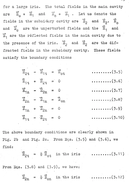
for a large iris. The total fields in the main cavity

are H + Hi and E „ + iL . Let us denote the

O J 0 I

— i.

fields in t h e - subsidiary cavity are E 2 and Eg. H Q

and E Q are the unperturbed fields and the and

E-j are the reflected fields in the main cavity due to

the presence of the iris. .S2 and H 2 are the

dif-t

fracted fields in the subsidary cavity. These fields

satisfy the boundary conditions

i t - i t = i t i... (3.5)

i t + i t = ' 0 ...(3-6)

H ln - _{i n} = 0 ...(3.7)

E 2n - E 1n E on ...,(3.8)'

E 1n + Xj2nIT' = 0 ...(3.9)

i t •E2t = 0 ...(3.10)

The above boundary conditions are clearly shown in

Fig. 2b and Fig. 2c. From Eqs. (3*5) and (3-6), we

find:

Hpt = i H 0t in ttLe iris ... (3.11)

From Eqs. (3.8) and (3.9), we have:

16

0 ’ 0

E on

E ? = H p = 0

(a)

4. V

0 +

^ . - +

H-■2n

n

Hr

(*)

2t

1n

E 2n

(o)

Pig. 2 Boundary conditions at the vicinity of

the iris. (a) Before■the iris is cut. (h) and

(c) Reflected and diffracted fields after the

4. SURFACE MAGNETIC*CHARGE & CURRENT DISTRIBUTIONS

In dealing with the discontinuities in elec­

tromagnetic fields which is physically impossible, it

is usually explained by assuming the presence of sur­

face distributions'of magnetic charge and current

whereby these discontinuities would be generated. In

other words, the.surface magnetic charge and current

distributions may be induced by the discontinuities i'fj

both E . and H. These quantities have no physical

meaning' but are mathematically important. Nor the sam

reason, the discontuities of the normal component of

the electric field and tangential component of the

magnetic field can be best analyzed by assuming the

formation of fictitious surface magnetic charge and

current densities in the coupling iris. Since the

subsidiary cavity■is initially unexcited, they are

considered"to be a complete set of the source of exci­

tation from which the fields in that cavity originates

Maxwell's'equations in three dimensions are given by:

V • H = P *

...( 4 . 1 )

18

(4.2)

and the continuity equation is given by

V - J * + f T - 0

(

.

)

where. and P are'the fictitious volume magnetic

current density and charge density respectively. . let

us now designate the fictitious surface charge density

If either Z * or 7J* is determined, the other one can'

he calculted hy Eq. (4.4).

If there are no electric currents and charges

present, the electromagnetic fields in the subsidiary

cavity will satisfy Maxwell's equations

by J * and the fictitious surface magnetic current

d

ensity by Z.t By analogy, to Eq. (4.3), K* and

satisfy the relation

7

.

ft* +

=

o

3t

(4.5)

19

We assume now a scalar potential <fi and a vector poten­

tial T so that

=

v x ft

4

7

dt

v r

4

8

as implied by Eqs. (4-5) and (4.6). Analogous to the

electric case, the scalar and the vector potentials

can be expressed by:

<j> (?)

-L

f J*cr) S I? ~r>l ds

S '

T u JJ / 1 (4.9)

ft (?) = -±- (( K*(r) $ l r ~ r ! ds

4K' J) (4.10)

S'

where r' is a source point on the iris; r is any

vector in the cavity from the center of the iris; S'

is the area of the iris; and g jr - r'| is the Green's

function

ilc Ir-r 'I I *** » I ' ©

g r - r' = —

r - r

By substituting Eqs. (4-9) and (4.10) into Eqs. (4.7)

and (4*8) and making use of the boundary conditions of

Eqs. (3.11) and (3.12) as obtained in Section 3, we

20

'2/1

-1 P

2 on,

Vr

A ( r k )

4 n K*(f>) x

v yg \ r - r

ds

H zt 2 Hct

M

at

v

_ !

4-TC J] dt

■5'

6

s'.V (4.12)

where . r^ is the field point in the iris, and

V r - K 7 7

21

In Eq.(4.12), the integrand of the first tern on the

right hand side is of the order of a? , while the second

term is of the order of d Z . Since the radius of the

iris is small compared with the wavelength, we may

neglect the first term 'of Eq. (4-.12). Moreover,-if we

also neglect the retardation in g |r - "r’l Eq. (4.12)

reduces to

= ~ 4 K ^ ... '

S'

where g' | rh- r'| = 1 / | r^- r 1

As an approximation, we may assume Hg-j. to be constant

over the iris and equal to 1- H Eq. (4.13) becomes

5' ■ (4.14)

It is well known that a constant electric field may be

produced by a uniform distribution of electric dipoles

on an ellipsoid, the dipoles having the same direction

as the field. The surface electric charge density will

be proportional to the product of the field and the

gradient of the surface electric dipole density. let

us apply the same idea to the magnetic field. The

desired surface magnetic charge density in the iris is

*

22

Up.on substituting Eq. (4 .15) into Eq. (4 .14) and

carrying out the integration, we can find that the

proportionality constant G is

c =

1

/ i t

2

.Consequently, the surface magnetic charge density is

*

Hot

%

7[z ( ol-Y<z)'/z

(4.16)

Erom the continuity equation of Eq. (4.-4), the surface

magnetic current is found to be

K*

= -

-k (a'-r'Y* ItL

-«.

f-

... . . (

.

)

71 d t

Bethe chooses a magnetic charge density on the iris to

create the proper The surface magnetic current

density K * creates a term in Eq. (4.11) of the order

2

of CL . Since this is presumably negligible as com­

pared with the actual normal component of "E2n = i ^ 0n ’

another magnetic current ,K'*is needed to maintain the

proper boundary condition for Eg^. on the iris with­

out disturbing the proper H 04- given by Eq. (4.12).

This is accomplished by means of a circulating current

with no divergence and hence no additional surface

magnetic charge density. Using the same technique as in

magnetic current density is obtained as

23

p/ £ T/ X Eon

^ ~- — --- jT • (4.1&)

Z n z (a7- p z)

In combining with. Eq. (4*17), the total surface magnetic

current density is

K * = K * + K'*

i ( r f - r l)A

]

n L bt z ( oE- t )

... (4.

T9)-Since the tangential component of the magnetic field'

and the nafinal component of the electric field over the

iris are given as

Hoi = 2

2a.o

Eon = 2 >2„ n r(nr £?40) + (2 f*e ^r( * % ) ■

n

0<

Consequently, Eq. (4.19) and Eq. (4.1(1) can be written

as

K

7' x n Y

Z(a-Y') *

/

(

.

)

'j *

Hao

^*j?°nrX fyo]

/ 7tz(cE-yt)'^ I u p r J

5. GENERAL EIELL SOLUTION.

The surface magnetic charge and current

density distribution over the coupling iris was obtained

in previous section. The next step is to determine

•the electromagnetic fields in the cavity coupling

system. As' stated before, the surface magnetic charge

and current densities may be considered as the only

sources of the excitation for the electromagnetic

fields in the subsidiary cavity. The fields in the

main cavity would not be the original fields alone but

are the resultant of the original wave and the re­

flected wave due to the opening of the iris on the

wall. In Section 4, we defined a scalar and a vector

potential

Substituting the values of J * and ( Eq.s. (4.21)

and (4.20) ) into Eqs.,(5.1) and (5.2) respectively,

we have

S'

( 5 . 2 )

25

4 -xn a. d t

+ z

f dt

nr *Gso • p $ i r - r ’l

S'

(

a*- - r,z)

Z \ '/« d s ]

(5.3)

R ( r , t ) = ~-L-3 j f z j i L o j j

t ,

(o?-

\ r

- r ' \ d s

+ Z J^°f{ n, x . ( L( a' -

’"Y ^ J

r

- r ' | Js ]

/ <f

i U T'CLO

T r x * r ( n r -£«o)

(az - r^)^

gj r - r ' l ot s

f ?' K nr (* r ‘

fka)

,

_ _ ,

,

, ---

n— S r - r

I

'J

(a *

-

r f ) M

(5.4)

Both Eq. (5.3) and Eq. (5-4) satisfy the M ax w e l l ’s'

equations

Ez ( r, t )

=

-V

x

fl ( f A )

(5.6)

It is seen that Eq. (5.5) and Eq. (5.6) are similar

in form to the general fields equations for a cavity

2 6

E

- EL To. E

t EEL -Pu jL ,

Ol 0 ^ 1

H ' — LEj Ha. GEL f* Gra .

p r f

We write the scalar potential as a product of a func­

tion of time and a function of space:

f ( f ' t )

Z, fy/t) tyjr).

Similarly, the vector potential:

ft ( r , t )

L yaz(t) Haj r )

Substituting Eqs. (5.7) and (5*8) into Eqs. ( 5 - 5 ) and

(5*6) respectively, we have

Ez ( r , t )

= X

CL ... ( 5 . 9 )

H A f . t )

= Z

(

.

)

where <fi'A and A# are 'the eigenfunctions satisfying 7*’z

the boundary conditions

n • = O ,

27

Prom Eq. (5*9)> we see that the irrotational electric

field does not appear in the expression. It is

now-necessary to give the proof_that the exclusion of P<*

terms from the general field equations for the sub­

sidiary cavity is justified. Y/e recall that the sur­

face magnetic charge- and current densities over the

iris are the only sources of excitation of the

sub-sidary cavity, and that there is no electric current

or charge present in V. Prom the M axwell’s equation

the time function or the expansion coefficient of P^<

is

v

In Section 2, Eq. (2.22) gives

V

s + s'

B y replacing J * by its known value ( Eq. (4*21) ),

Eg;. (5.11) becomes

/

7Tz/l 'kk

~t ____

f vr JJ

(az - r^)'^

r> • n r y tip* d s j

— .(5.12)

Again from Eq. (2.16) in Section 2, we have

tie

/ a v

f ~kaz ra*.

" f J * - H ^ c t v

v i x E - H « Z ^S

sts'

With the aid of the conditions:

J* = 0 in V

n x E = 0 on S

n x E = ]<* on S',

^ it

Eq. (5-15) can be reduced to:

( 5 . 1 3 )

29

Bor H aJ r ) = (r)_, we finally get

' / " J F * = - f[icf -/ t i & ) * ... (5.14a)

5'

Since the value of Kr* is given "by Eq.(4.20) in

Section 4, the right hand side of Eq. (5*14a) may "be

expanded into

_ i{ K* ■ A'a*( % ) d s

S'

+ ( *r * f c j a* - r * y * ds f St. &

~ j r _&»■ (f r YYt,{?%■ £ » p • ,

-a ^ y, ( a.1 - rA ) \

- ZL

7Ir

o<

z n

(a* - rfZ)

^

( 5 - H h )

By solving the linear differential equation of Eq.

(5.14a ) , we can determine the expansion coefficient

r aX/ whereby sa A will be obtained

d Yclz

= I F ' < 5 - 1 5 ’

30 ,

coordinates Taut depends on the time dependent expan­

sion coefficients of the fields in the main cavity.

This equation is well known as a forced oscillation

differential equation as it must he.

As shown in Eqs. (5*12) and (5*H a ) , the

expansion coefficients depend on the eigenfunctions

A ^ s and s of possible modes in the subsidiary

cavity. In turn, -A^s and s depend upon the

shape, construction of the cavity, its boundary con­

ditions, and the frequencies of the fields in the main

cavity. If the shape and the boundary conditions of

the subsidiary cavity are specified, the eigenfunctions^

A'azs and 5^ s will be obtained, so as the expansion

coefficients ra z , s az and q ^ . - Substituting these

'known values into Eq. (5.9) and Eq. (5.10), we shall

h a v e .a complete solution for the field configuration

in the subsidiary cavity. In the like manner, we shall

obtain the reflected fields in the main cavity only

due to the presence of the fictitious surface magnetic

charge and current in the iris. Then applying the

superposition method, we shall acquire the total fields

in the main cavity.

The problem in determining the field, con­

31

solved. In the next chapter, we shall work out an

example to illustrate the application of the solutions.

In the meantime, the proper procedure and technique in

solving a practical problem will be given in detail.

The solution obtained in the last two chapters are

also applicable to the cavity-waveguide system coupled

7. EXAMPLE

The cavity-coupling system consists o f a main

cavity of dimensions 1%, , I'j, and <4, , and a subsidary

cavity of dimensions JL*Z > l y z > and . These two

cavities are resonating at about the same frequency and

are coupled through a circular iris of radius 'a. ’.

The iris is located at the centre of the common wall

whose thickness is negligible. The schematical diagram

of this system is shown in Figure 4.. Now let us assume

I c o t

that only mode of the £ time dependence is

being excited in the main cavit,/. Regardless of the

sources of excitation, the fields are given by:

(

v

)

B j n t ^ k b

■+ . Q-z. B & /Q/syi

7

o

Pig. 4 Schematical diagram of the

cavity-coupling. system.

f

X

2

34

•—* _> jM * >

Ea, = A £ ^ J L Jjst 5J_L Airt, HJL ... (6 .3 )

/*, A

-i

where A and B are arbitrary constants and

z

_ f 3 r t f

f ix ^

f ^

\z

«/ ~ -r- +

t

L

-+

c*i.‘ _U'/

Prom now on, it is convenient to translate the origin

of'the coordinate system to a position so that it co­

incides with the centre of the iris and the xy-plane

coincides with the plane of the iris. It is shown in

Pigure 5. The new coordinates ( x ' , y * , and z' ) and

the old coordinates ( x, y, and z ) systems are related'

by •

X =

x ' •+

t = f + h / t

-Z = Z '

+

With the new set of coordinates, Eqs. (6.1), (6.2), and

(6.3) now become

35

Ta, £ * = - /2ZL } m

w i a * r ~z,

•

(

.

)

At the centre of the iris or at O' (x1 = y ’ = z' = 0)

_» _ / 37lZ \

S« H «

Of, = - a t B ( J J L . } g/"*

Xl /'

'fa./ B a., — 0

Since the iris is assumed'small compared to the wave­

length, the fields incident on it will be considered

constant throughout

3 At*' ^ 3 3rt 1 J vt

H ‘ “ - a% 1 > 1 4 1 + - T T 1 e

(6.7)

E

0

—

O

(

6

.

8

)

determine the fictitious magnetic charges and currents

b y applying Eq. (5.21) and (5.22) in Section 5.

r t * r f r j.\ = L [ J A l L _ 3 3 ? r a * ‘ T ' e Jcot

/

**1 4 4 4

4a:, J («"

-... ( 6 . 9 )

T2*/z:. l\ _ _ 4 ^ f '3 6co ^

K ( n t ) - j e I J J J l .

(

.

)

If we neglect the retardation, the scalar potential

due to the fictitious magnetic charges is :

9

=

* f 1

1

lK aX- * r *

After performing the integration over the iris, we hove

in, -kp,

(

.

)

Similarly, the vector potential due to presence of the

fictitious magnetic current is :

* < ’ ■ • > ■ -j * l

’ ,..(6.12)

She next step is to evaluate the time co­

37

3 a J F __________

7r

a 'iw,

I

/ /

j

/ / ' ^Xr^-Z, K.a, kf}t

T z 7r u - i , I 7 " T ~ 7 3 " “ 3 ~ I e '

I >)

From Eq. (5. H a ) in Section 5, we have

f

6 j j r

+

i l r«i

=

-

'

4

...(

6

.

14

)

Since z

O'

-

;3nco\ A

8

r f s

-~ y - T — / -nrr*. — 7-7 - / ~ -f ) <?*

.

<? ' 4 4 4 , T r / ^ ^ J £

The integral on the right-hand side of Eq. (6.14) can

be e a s i l y evaluated ;

ff

a

J

-

3c"

f - -

- 5

s je° f

jj

K ■

/£&

Jz ~ —/£

, 4

w)J <2 •

5' r

By substituting this value into Eq. (6.14), we have

.6

2%z + i z r - 3 1

-

^ /

&

m

^ “7 - f-T7J - - V <T .

/ - 4 14 tt^/j

By solving this linear differential equation, we find :

= - -- — ---- — I 3<o, fl ft s Y rJ ( ^ r ^ ) t ,

3>3

or

.. 5

icot

#coajta 6 _____ <• _ _3_\1 /)

'5Jjue (&>at + <*>) d 00 A, A^*, ltfyt •*

...( 6 . 1 5 )

where

k co ~ ^dz

The time coefficient for the eolenoidal magnetic field

is :

5*a, aftt

a f

= “7

/ 5" jcot ycogcoa e

/$JjOZ ( <Vat +cu)Aco

£

iAOjt

(e

In case of

co —*■ cu

c Jco-t

r .

2<n e

3co t

s

'a*, = “

K j / T e A W

Xt, h,ii,

r Y

j

...( 6 . 1 7 )

r Jcot

-

-j

y # J/ie A < o t U f a rfy/J '

39

Now, we assume further that only T E . ^ mode

can be excited in the subsidiary cavity. The fields

in the subsidary cavity are

4 - y - W - « ) V 4 e j M t - ,)

AWj.ii j.Zf'fea., ~K"kj$t

[ s * T ~ r ~ / r ^ ( - o f f ? ) ; < * , S i L

1

444\

A, 27

A.

V/xA,/ ' /x, * / . . . A . . .(6 .19)

( _ 4 2 L _ - _ e _ )

' 4 A 4 4 * A,

4-[ « „ _ Z L _ t J L ) A n 1 ? L

i-uip* ‘ A . * ' A

- tfg — CxW / -f - f ) x?x(*. -A. 1

A, ha

Ax

)

A*

(

6

.

20

)

%, 4 = - / a: 4 : / / L + _ s _ ) V w V e ^ ()

4 , a * }

[ t V ^ + - f ) ^ ) 1 ■

A? & ) t 11 .,.(6.21)

The total fields in the main cavity are now the sum

of the incident fields plus the reflected fields due

4 0

so designed that at frequency _t> 33L_2j( only TE,A1 mode can_{j 301}

be excited. The field configuration remains unchanged

but the amplitude ( or the time dependent expansion

coefficients ) differ slightly from the unperturbed

amplitude.

Si, Ha,

=

a

5

Q 2 jACoi

j'Ot

g y ; nip,

a,x faJL - jSjAt f.

1 Jty *>

3 m ' , 3n\ -ni'

j ^ ~ r~

+

V/

a.

a . 6 v =

h

«/

xun (-AlUL + J f a yd-^v

[ A *>>

ft + 3 d 3 f

(

dt - A L £

-- a,

A i y

TV

i t

U

CdV

U, & at _-

I *

z, ■y/

6cozo f

<-tl

f\

rr

fi ' u

3nx' 3tt v- —

Z

5

)

i fat

A

yCMd

ig.

^ ydivu 7fZ' 1 ii, •

3 y.

f a !

c —

^ ydU/i 7TZ' )

4 J KZ'

ig,

-(

.

)

(6.23)

0]

e >ut

A. Vector and Scalar Functions

In any closed region V bounded by a regular

surface S , we may define an arbitrary piecewise con­

tinuous vector function and an arbitrary piecewise con­

tinuous scalar function by setting up two complete sets

of orthogonal eigenfunctions for each of them. Each

of-these satisfies the wave equation and its corresponding

boundary conditions. For the vector function, we have

f T Kf V " ° (in V ) (A. 1a)

.

% x Wp

o

n • n

o

and

* 4 — O (in V ) ...(A.2a)

n

<£j. = O

For the scalar function, we have.

41

42

V f* + = 0 ( in V )... (A . 3a)

Y * = 0 ( on S (A.3b)

and

tp * ~ 0 ( in Y ) ... (A. 4a)

^ ( on S ) ... (A. 4b)

where k^ , k^ , k ^ , and ly are the eigenvalues of

the eigenfunctions ^ ^ , and ^ res­

pectively; p, q , c< , and are integers ( = 0, .1 ,• 2,

3, .); n is a unit normal vector on S.

Green's theorem states that if two vector

functions, and , are continuous in a closed

region of- space V' bounded by a rdgular surface S,

we' can write

[fSr ‘( 7 X 7 x ^ ) - ^ • ( v x v x ' ^ ) j A v v

= [ J- x' V x ^ - Ify, X V x ^ ] . n d s

s

... ( A . 5)

Expanding V x V X terms and applying the divergence

theorem, we get:

\\\

-S?

-v*yf ] l v

V

[ V f V - i , - $ t 7 -wr y n - [ Z r - ( H w . f , (A>6)

43

Prom Eq.. (A. 1a) and Eq. (A. 2a), we have

„ ^ r $f - v ^ r - ( -I; - 4 ) • 4 ,

Eor k = lc , the volume integral in Eq.. (A. 6) vanishes,

£T M.

Further applying the boundary conditions, Eq. (A.6)

reduces to

jT j

x s^)}

=

jjj

dv

Since the fields are confined in an enclosed region

bounded by a surface S, the integrand in Eq. (A.7)

must equal . to zero, i.e.,

( v- $p) *n - • ( n X & j X V X - n

■■= 0

Since none of the normal component of e$ch term in the \

above expression vanishes on the surface S, it must be

V r v * f - f y x v x y . - 0 (A>8)

From the vector identity, we may put

V ' f

v-

) =

v-WfV-$2 -t

■ v*

44

we have

...(A.10)

Upon substracting Eq. (A.10) from Eq. (A.9), we again

get

v • (iPr v-$f ) - v- ( $ f V - w f )

= ^ * V z$f - $ .

- ( t f - (ju11) .

The volume integral of the right hand side of Eq.(A.11)

-equals to zero if = k^. Using the divergence

theorem, the volume integral of the left hand side is

v ^

7

v- ( $j v- WpjJJv

jjn-[iPfr-gf-$/ v-ii'f]c/s

V 5

or

n

~r ' ' T ' ” ■

₅

n

•

typ ( V - d s -

n-

( v - ^ ) ds

for n * ^ = 0 on the surface S. Since . n , * ^ ^ 0 on S,

V ^ ) (A. 1 2)

Hence, we obtain from Eq. (A.8) that

X V X % = 0

45

By the use of Eqs. (A.12), (A.2b) and (A.13), Eq. (A.5)

reduces to

^ • ( 7 X 7 X ^ ) - l ^ f 7 X 7 X ^ ) ] V v 2 Q

V

or

nPp-C V K V X ~ ( V x V X IPf) = o

(A.14)

Now let us consider Eq. (A.12) and (A.13)

carefully. Since 3Z^ j ^ ^ 0 in V or on S, ^

must be a curl of a vector function and , on the

other hand, may either be a gradient of a scalar

function or be that its curl is proportional to 2^ .

if ^ and ^ also have to satisfy Eq. (A.14), the

solution is

'tf&f = ^

= V X

and k = k .

^ ir

If we let k = k = k a (a, =>1, 2, 3, .... )

— V X ^ '.(A. 15a)

ka. 'Wa, = V.X (A. 15b)

For k 7^ k , 3^ and ^ will no longer

P q / n

have any correlation between them. It is quite obvious

corresponding boundary conditions which distinguishable/

mark their different characteristics. Let us consider

the boundary condition n x Uy, = 0 from Eq. (A.1b).

Its surface integral will also he zero since the

tangential component on S vanishes,

i.,e.,-\\ n

x ijL

ds = o

5

But

n

5

A

§f ds

= jff

VX §f d v = 0

on S or in V. Hence

V

possible solution of is

ip

=

' ' ' . ...(A.16)

By using similar technique for the boundary condition

= 0, we obtain /

j l " 71 X 7 X Wj d s = j H &X V X dLv = r O

S V

Nov/ we can equate

V x V x & = 0

f

Since V X V X = V(V')~ V*' and f £ % & z-O , it becomes

o f f

V ( V ■

Sf ) - 7^

o

How we see that is a gradient of a scalar function.

If k 4 0 and 4 0 in V, then the solution for

47

in general is

(A.17)

Y/e have now proved that in a closed region hounded by

a regular surface, a piecewise continuous field vector

can always be expressed by an irrotational and a

solenoidal function with corresponding boundary condi­

tions. When two vector functions of different boundary

conditions are presented in that closed region, one

can be determined by the curl of the other for equal

eigenvalues. For unequal eigenvalues, these functions

are measured by a gradient of scalar functions. It is

also obvious as shown in the proof that although we

have defined four groups of orthogonal eigenfunctions,

namely, ^ ^ , and <p , the last two /nay be

derived from the first two.

B. Orthogonality

Yfe are satisfied that the..electric field as

well as the magnetic field are orthogonal, and that in

a complete expansion of^electromagnetic fields in a

of orthogonal functions. But, for the series expansions

of Eqs. (2.1) and (2.2) in Section .2 to be valid, the

orthogonality of these functions must be shown. Prom

the vector relation, we can write

V ' [ £t,*(VxE«,)3 = ( V x £ 6 )-(V*£a.) - E ^ V X (v x e a)

...(B.1 a)

V -f ( 7 x Ei)] = ( V x Bo,)' ( 7 X E b) - £ • V X ( V X Eb)

...(B.1b)

Iheir difference gives

(B.2)

V' [ £6

(VX U ) ]

V- [Ea, x ( V X E b) ]

= Kl' V x (V.XEb) - Eb .

vx (VXE^)

Since 7 X V * 4 =

' v ( v - -

V ZE^

V ' Ect, — O f

V*Ea, -f il E o ^ - 0

Eq.-(B.2) reduces to

7- [ E b X ( V X U ) J - V'[Ec,x(Vxeb)J = (il- A*) E«,-Eb

Upon taking volume integral on both sides and using the

divergence theorem, we obtain

= . / / f

v s

- “ka. \ \ n

[Eb X Ha.

Ea. X Hb] ds

■5

Owing to the vector identities

'n-

x

• ( n x

)

71. Bb X Ha, = H a ‘ ( n x E b)

and the boundary conditions, the surface integral in

Eq. (B.3) equals to zero. If a ^ b, It ^ k ,

>(B>4)

If a = b , Eq. (B.1a) or Eq. (B.1b) becomes

V' [ L

(

E

)] = (vxE4.)'(vx£a.) -£«.-rx (rxea.)

P rom the relations of Eqs. (2.5a) and (2.5b)» we have

7- [E«x (vx£a)]

ilHi - it El

As before, the volume integral of the left hand side

of the above expression vanishes. The volume integral

of the right hand side is

• C /// ( H t - EJt) d v = 0 V

Hence,

v

H i c L v - JjT e £ d v - o

V

■

V

where C is an arbitrary constant. Through the

similar procedure as above, we (have, the similar

results for the functions H a and H b . After the

normalization, we finally have

50

( B . 7 )

Snd

5.* =

/ if

a = b

Now, let us consider

7

- (ft V

fa)

= 17

fa - 7 f t ~

%

7*

ft

Because of Eq. (2.6t>), it can be rewitten as

■7 '(fa 7 f t)

=

V fa ' 7

ft - ^ fa ft

(B.8)

By interchanging the roles of

'fa

^ b

get

7 ‘{ft 7 % )

7

fa-V

ft- itfafk

,

.

'

(B.9)

The substraction of Eq. (B.8) from Eq. (B.9) gives

{-it -■ i t ) f a f t = 7 - ( f a 7 f b) - V ■( f t 7 f a )

Ag a i n taking volume integration on both sides and

using the divergence theorem on the right hand side,

we have

( £

it) ( ( ( iv

J[[[

‘Ciinfii) -

(fb vfjldv

V

V

51

Since ^ =

'fb -

( H

it) \\\ % f h<Lv

v

If a

^

\ \ \ ' % % < t v = 0 (B. 10)

V

Prom Eqs. (B.8) and (2.6a), we obtain

v ' (faFb)

=

^b ( kcfcc'h - ibfc,fb)

Using the same integration technique as before,

% V * ( % h

)

=

-

V V V

* F b

*f*. &

-f^cLv- ib ^ % f b<lv

6 y y,

P or the boundary condition ^ = 0 on S,

-£«. Pa - Pb -

i b§\

1/ V

If a / b,

'fa.'j'b^v-

V

? a Pb = 0 ( B . 1 1 )

V

If a = b,

1 H I

-V

V

After normalization,

?;