University of Windsor University of Windsor
Scholarship at UWindsor
Scholarship at UWindsor
Electronic Theses and Dissertations Theses, Dissertations, and Major Papers
Fall 2017
Analysis of Fluid Queues Using Level Crossing Methods ID: 11563
Analysis of Fluid Queues Using Level Crossing Methods ID: 11563
Chi Ho Cheung University of Windsor
Follow this and additional works at: https://scholar.uwindsor.ca/etd Part of the Physical Sciences and Mathematics Commons
Recommended Citation Recommended Citation
Cheung, Chi Ho, "Analysis of Fluid Queues Using Level Crossing Methods ID: 11563" (2017). Electronic Theses and Dissertations. 7337.
https://scholar.uwindsor.ca/etd/7337
This online database contains the full-text of PhD dissertations and Masters’ theses of University of Windsor students from 1954 forward. These documents are made available for personal study and research purposes only, in accordance with the Canadian Copyright Act and the Creative Commons license—CC BY-NC-ND (Attribution, Non-Commercial, No Derivative Works). Under this license, works must always be attributed to the copyright holder (original author), cannot be used for any commercial purposes, and may not be altered. Any other use would require the permission of the copyright holder. Students may inquire about withdrawing their dissertation and/or thesis from this database. For additional inquiries, please contact the repository administrator via email
,
ANALYSIS OF FLUID QUEUES USING LEVEL CROSSING METHODS
by
Chi Ho Cheung
A Dissertation
submitted to the Faculty of Graduate Studies through the Department of Mathematics and Statistics
in Partial Fulfillment of the Requirements for the Degree of Doctor of Philosophy at the
University of Windsor
Windsor, Ontario, Canada
2017
c
Analysis of Fluid Queues Using Level Crossing Methods
by
Chi Ho Cheung
APPROVED BY:
D. Woolford, External Examiner University of Western Ontario
S. Goodwin
School of Computer Science
A. Hussein
Department of Mathematics and Statistics
S. Paul
Department of Mathematics and Statistics
P. Brill, Co-Advisor
Department of Mathematics and Statistics
M. Hlynka, Co-Advisor
Department of Mathematics and Statistics
DECLARATION OF ORIGINALITY
I hereby certify that I am the sole author of this thesis and that no part of this thesis
has been published or submitted for publication.
I certify that, to the best of my knowledge, my thesis does not infringe upon anyones
copyright nor violate any proprietary rights and that any ideas, techniques, quotations,
or any other material from the work of other people included in my thesis, published or
otherwise, are fully acknowledged in accordance with the standard referencing practices.
Furthermore, to the extent that I have included copyrighted material that surpasses
the bounds of fair dealing within the meaning of the Canada Copyright Act, I certify
that I have obtained a written permission from the copyright owner(s) to include such
material(s) in my thesis and have included copies of such copyright clearances to my
appendix.
I declare that this is a true copy of my thesis, including any final revisions, as approved
by my thesis committee and the Graduate Studies office, and that this thesis has not
ABSTRACT
This dissertation is concerned with the application of the level crossing method on fluid
queues driven by a background process. The basic assumption of the fluid queue in this
thesis is that during the busy period of the driving process, the fluid content fills at net
rate r1, and during the idle period of the driving process, the fluid content, if
positive-valued, empties at a rate r2. Moreover, nonempty fluid content, leaks continuously at a
rate r2. The fluid models considered are: the fluid queue driven by an M/G/1 queue in
Chapter 2, the fluid queue driven by an M/G/1 queue with net input and leaking rate depending on fluid level, and type of arrivals in the drivingM/G/1 queue, in chapter 3, and the fluid queue driven by anM/G/1 queue with upward fluid jumps in Chapter 4. In
addition, a triangle diagram has been introduced in this thesis as a technique to visualize
the proportion of time that the content of the fluid queue is increasing or decreasing
during nonempty cycles. Finally, we provide several examples on how the probability
density function of the fluid level is related to the probability density function of the
ACKNOWLEDGMENTS
I would like to thank my supervisors Dr. Myron Hlynka and Dr. Percy Brill for all I
have learned from them and for their continuous support in every stage of this
disser-tation. This dissertation would not have happened without their Hlynka’s and Brill’s
encouragment.
At the University of Windsor, I would like to thank Dr. Scott Goodwin in Department
of Computer Science, Dr. Sudhir Paul, and Dr. Abdulkadir Hussein in Department
of Mathematics and Statistics for agreeing to serve on my dissertation committee, for
reading my thesis, and for providing detailed comments on the thesis. Outside the
University of Windsor, I would like to thank Dr. Douglas Woolford in Department
of Statistical and Actuarial Sciences at Western University for agreeing to serve as an
extremal examiner on my dissertation committee.
In addition, I would like to thank for Dr. Betty Jo Barrett in Department of Women’s
and Gender Studies, Dr. Percy Brill in the Department of Mathematics and Statistics,
Dr. Amy Fitzgerald in the Department of Sociology, Anthropology, and Criminology /
Great Lakes Institute for Environmental Research, and Dr. Nazim Habibov in School of
Social Work for the research scholarship during my time at the University of Windsor.
Last but not least, I would like to thank all faculty, staff members, and graduate students
in Department of Mathematics and Statistics, University of Windsor for helping me in
TABLE OF CONTENTS
Page
DECLARATION OF ORIGINALITY iii
ABSTRACT iv
ACKNOWLEDGEMENTS v
LIST OF TABLES x
LIST OF FIGURES xi
LIST OF ABBREVIATIONS AND SYMBOLS xiii
1 Introduction 1
1.1 Introduction . . . 1
1.2 Literature review of fluid queues driven by Markovian process . . . 3
1.2.1 Stationary distribution of fluid queue . . . 3
1.2.2 New contributions . . . 6
1.2.3 Potential applications . . . 6
1.3 Elementary properties of renewal processes . . . 7
1.4 Applications of level crossing methods on fluid queues . . . 11
1.4.1 Example 1: Buffer level of fluid queue driven by a single On/Off source . . . 11
1.4.2 Example 2: Distribution of the fluid level of the fluid queue with a finite capacity R . . . 16
1.5 Conclusion . . . 23
2 Infinite capacity fluid system 24 2.1 Fluid queue driven by an M/G/1 queue . . . 25
2.1.1 Introduction . . . 25
2.1.2 Terminology of the fluid queue . . . 26
2.1.3 Definition of the probability density function of the fluid level . . 27
2.1.4 Stability condition of the fluid queue . . . 28
2.1.5 Expected values of the fluid queue . . . 30
2.2 Probability distribution of the fluid level . . . 32
2.2.1 Downcrossing and upcrossing rates of level x . . . 32
2.2.2 Triangle diagram . . . 33
2.2.3 Level-crossing equations . . . 35
2.2.4 Beneˇs-like series for PDF of fluid level . . . 36
2.3 Laplace-Stieltjes transform . . . 39
2.3.1 Introduction . . . 39
2.3.2 Laplace-Stieltjes transform of the fluid level . . . 40
2.3.3 Laplace-Stieltjes transform of the wet period . . . 42
2.4 Number of tagged arrivals, arrivals served, and peaks in a wet period . . 46
2.4.1 Number of tagged arrivals in a fluid wet cycle . . . 46
2.4.2 Number of arrivals served in a wet cycle . . . 47
2.4.3 Number of peaks in a wet cycle . . . 49
2.5 Numerical illustration . . . 51
2.5.1 Simulation . . . 51
2.6 Relating probability distributions of the driving and fluid queues . . . 52
2.6.1 Fluid queue driven by modifiedM/G/1 queue . . . 54
2.6.2 Fluid queue driven by an M/M/1/1 queue . . . 57
3.1 Fluid queue with leaking rate depending on fluid level . . . 63
3.1.1 Introduction . . . 63
3.1.2 Level-crossing equation . . . 64
3.1.3 Probability distribution of fluid level . . . 67
3.1.4 Mapping the integral equation of the probability density function of the workload of M/M/r(·) and the fluid level . . . 72
3.2 Fluid queue with different leaking rates . . . 75
3.2.1 Introduction . . . 75
3.2.2 Level-crossing equation . . . 76
3.2.3 Probability distribution of fluid level . . . 84
3.2.4 Expected value of fluid level . . . 88
3.2.5 Simulation of fluid level . . . 89
4 Fluid queue with jump fluid inputs 91 4.1 Model I: Fluid queue with irregular arrivals . . . 92
4.1.1 Motivation and introduction . . . 92
4.1.2 Level crossing equations for f1(x), f2(x), andf(x) . . . 94
4.1.3 Laplace-Stieltjes transform of fluid level . . . 98
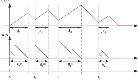
4.1.4 Mapping the sample path of the virtual waiting time of anM/G/1 with exceptional service for zero-wait arrivals to the sample path of the fluid level of the fluid queue with irregular arrivals . . . 101
4.2 Model II: Fluid queue with variant . . . 103
5 Summary of chapters 108 5.1 Summary of Chapter 1 . . . 108
5.2 Summary of Chapter 2 . . . 109
5.3 Summary of Chapter 3 . . . 109
5.4 Summary of Chapter 4 . . . 110
Reference/bibliography 119
LIST OF TABLES
Page
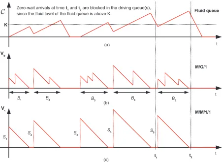
2.1 Simulation results of fluid queue expected values . . . 52
LIST OF FIGURES
Page
1.1 A sample path of fluid level and driving process of ordinary fluid queue. (a) {Z(t)}t≥0, (b) {C(t)}t≥0, (c) {C(R)(t)}t≥0. . . 18
1.2 The sample paths of the processes: (a) {Z(t)}t≥0, (b) {C(t)}t≥0, (c) {C(R)(t)}
t≥0. . . 21
2.1 (a) A typical sample path of fluid level. (b) The states of the fluid queue. (c) The states of the drivingM/G/1 queue. . . 27
2.2 Composition of a single wet cycle . . . 31
2.3 (a) A typical sample path of fluid level. (b) A corresponding sample path of fluid level. . . 33
2.4 Triangle diagram of the fluid level . . . 34
2.5 (a) Two successive wet periods of the fluid queue; (b) Life time of the sub-wet periods corresponding to (a). . . 43
2.6 Sample path of the fluid level and waiting time. . . 55
2.7 Sample paths of the fluid level and corresponding virtual waiting time of the driving queue: Diagrams (a), (b) and (c) are discussed below. . . 58
3.1 A typical sample path of the fluid queue with leaking rate depending on fluid level and the virtual waiting time of the driving queue. Top corresponds to the fluid queue. Bottom corresponds to the drivingM/G/1 queue. . . 64
3.2 (a) a sample path of {Z(t)}t≥0, (b) a sample path of {C(t), Z(t)}t≥0, (c) a
sample path of{C(t), Z(t) = 2}t≥0, and (d) a sample path of{C(t), Z(t) =
1}t≥0. . . 69
3.3 Laplace-Stieltjes transform of the pdf of the fluid level. Driving queue is M/M/1. . . 72
3.5 (a) a sample path of {C(t)}t≥0, (b) a sample path of {C(t), Z(t) = 2}t≥0,
(c) a sample path of{C(t) |Z(t) = 2}t≥0. . . 74
3.6 A sample path of the fluid queue and the drivingM/G/1 queue . . . 76
3.7 Sheet and line 0 diagram . . . 78
3.8 Triangle diagrams for a typical sample path . . . 82
3.9 Laplace transform of fluid level . . . 86
3.10 Laplace transform of fluid level . . . 86
3.11 Approximated probability density functions corresponding to the LSTs in Figure 3.9 . . . 87
3.12 Approximated probability density functions corresponding to the LSTs in Figure 3.10 . . . 87
4.1 A sample path of fluid queue with irregular arrival . . . 93
4.2 A sample path of virtual waiting time of anM/G/1 queue with exceptional service for zero-wait arrivals . . . 101
4.3 A sample path of virtual waiting time of anM/G/1 queue with exceptional service for zero-wait arrivals . . . 102
4.4 A sample path of fluid level of the fluid queue . . . 102
4.5 A sample path of fluid queue with irregular arrival . . . 104
LIST OF ABBREVIATIONS AND SYMBOLS
Following is a collection of the abbreviations and notations used frequently and
consis-tently throughout the dissertation.
Abbreviation Description
cdf Cumulative distribution function
ccdf Complementary cumulative distribution function
eq Equation
LC Level-crossing method
pdf Probability distribution function
Symbol Description
A Activity period of fluid queue
AT Duration of activity periods of fluid queue in a wet cycle
B Busy period of driving queue
B(x) Cumulative distribution function ofM/G/1 queue busy
pe-riod
Bc Busy cycle of driving queue
C Fluid level of fluid queue
Dt(x) Number of downcrossings of level x during (0, t)
Exp(λ) Exponential random variable with parameter λ
E Empty period of fluid queue
I Idle period of driving queue
Np Number of peaks within a fluid wet cycle φ(t) States of the fluid queue
P oiss(λ) Poisson random variable with parameter λ r1 Net input rate for fluid queue
r2, r3 Leaking rates for fluid queue S Silence period of fluid queue
ST Duration of silence periods of fluid queue in a wet cycle Ut(x) Number of upcrossings of level xduring (0, t)
µ Service rate for driving queue W Waiting time of an M/G/1 queue W Wet period of fluid queue
Wc Wet cycle of fluid queue
Chapter 1
Introduction
1.1
Introduction
Waiting in line is a phenomenon in daily life. All of us encounter certain types of waiting
lines before receiving service, such as waiting lines at Tim Hortons to buy a coffee, in
a hospital (or outside a hospital) to access a healthcare service, at the border to enter
another country, or on the phone when calling customer support. Waiting in line is
annoying for most of us; unfortunately, no one can escape waiting in line. However, we
can use a mathematical model to study the characteristics of waiting lines to reduce the
delay time and to improve the efficiency of the service.
A mathematical model used to study the characteristics of waiting time phenomena is
called a queueing model and was first studied by Erlang [17] in 1909. The original paper
by Erlang was intended to study traffic in telecommunications. Since then, hundreds
of queueing papers are published each year. In traditional queueing theory, a queueing
model consists of a single server that provides service to individual arrivals. The
1.2. Introduction
or may not need to wait in line before receiving service. For this single server queueing
model, we are interested in the experience of arrivals in terms of delay and service time.
The assumptions of queueing models can be summarized in the notation A/B/n/m
in-troduced by Kendall [23], where A and B correspond to the distribution of interarrival
time and service time, n is the number of servers for the queueing model, and m is the
capacity of the system.
The queueing models we have mentioned so far can be classified as discrete state space
queueing models where the states are the numbers of customers in the system. In discrete
state space queueing models, some characteristics of the queueing model can be analyzed
by a discrete event. For instance, using the fact that the waiting time and service time
are attached on individual arrivals, we can find the distribution of the busy period by
adding up each individual’s service time in a busy cycle, where the busy cycle is defined
as the time between of two consecutive arrivals’ waiting times being equal to 0.
Recently, continuous state space queueing models, such as the fluid queue, have received more attention from researchers. In a fluid queue, arrivals are too small to distinguish
between them in the fluid system. Thus, it is easier to consider arrivals as continuous fluid
that enters and exits the fluid queue. One example of a fluid queue has arrivals which
enter and leave the queue with rates modulated by a background Markovian random
environment process such as a birth-death processes,G/G/1 queue, or vacation queueing
model ([42]). Researchers usually refer to capacity of the queue as the fluid content. In
this dissertation, we focus on infinite-capacity and finite fluid content queues driven by
1.2. Literature review of fluid queues driven by Markovian process
1.2
Literature review of fluid queues driven by
Marko-vian process
1.2.1
Stationary distribution of fluid queue
Consider an infinite fluid content queue with a background Markovian random process
(or environment process) with finite state space. The fluid content fills and empties at
rates that are modulated by the background Markovian random process, which is not
necessary observable. Denote by C(t) the fluid level at time t (≥ 0), and by Z(t) ∈
{1,2,3, . . .} the states of the continuous time random process which makes the joint
process {C(t), Z(t)}t≥0 a Markov process. The characteristics of the fluid queue can be
summarized as follows:
dC(t)
dt =
rZ(t), C(t)>0,
max(0, rZ(t)), C(t) = 0.
(1.1)
where rZ(t) < ∞ is the net input rate of the fluid queue at time t. Using Kulkarni’s
terminology [25], we may refer to the {C(t)}t≥0 process as a fluid process driven by the
background Markov renewal process {Z(t)}t≥0.
Consider a Markov renewal process{Z(t)}t≥0 with the states of anM/G/1 queue defined
as follows
Z(t) =
1 if the server of the M/G/1 queue is busy,
2 if the server of the M/G/1 queue is idle.
(1.2)
The {C(t)}t≥0 process is referred to as a fluid queue driven by an M/G/1 queue [4, 44].
Virtamo and Norros [44] study the steady-state distribution of the fluid level using a
expo-1.2. Literature review of fluid queues driven by Markovian process
nentially distributed with rate µ (i.e. the net input rate of the fluid queue is modulated
by an M/G/1 queue). Adan and Resing [4] re-investigate the model and derive the
Laplace-Stieltjes transform (henceforth LST) of the steady-state distribution of the level
of fluid queue with net input rate r1 = 1 and leaking rater2 =−1 driven by an M/G/1
queue, using a regenerative processes approach1.
More precisely, let {Bn}n≥1 be a sequence of busy periods, and{In}n≥1 be a sequence of
idle periods of anM/G/1 queue (see ([45]) for definition of busy and idle periods). Adan
and Resing consider B1, I1, B2, I2, . . . as an alternating renewal process, the fluid level
Cn at the beginning of the nth busy periodBn satisfies the well known Lindley recursion
(see [12, p. 3 eq (1.1)] and [18, p.14, eq (1.5)] for the details on Lindley recursion)
Cn+1 = (0, Cn+Bn−In)+, n = 1,2, . . . . (1.3)
Observation 1.2.1. Consider Cn to be the waiting time of the nth arrival, Bn to be the
service time of the nth arrival, and In to be the interarrival time betweennth and(n+ 1)st
arrivals of an M/G/1 queue, then (1.3) is the Lindley recursion for an virtual waiting time of the M/G/1queue. Thus, expression (1.3) suggests that the characteristics of the fluid queue can be achieved by understanding the characteristics of the M/G/1 queue.
Laplace-Stieltjes transform of steady-state distribution of the fluid level
Let Be(s) := R0∞e−sxdP[B ≤ x] be the LST of the probability density function (pdf) of the busy period of an M/G/1 queue which is driving the fluid queue, and Ce(s) :=
R∞
0−e−sxdP[C ≤ x] be the LST2 of the pdf of the fluid level of the fluid queue C. Adan
and Resing derive the LST of the pdf of the fluid level of the fluid queue driven by an
1
It turns out that using renewal theory, the expected fluid cycle and the expected number of peaks within a fluid cycle can be easily achieved.
2
We use 0− in the lower limit of the integral of the LST to indicate that there has a point mass at
1.2. Literature review of fluid queues driven by Markovian process
M/G/1 queue in [4, eq. (3), p. 172] as
e
C(s) =
1−λE[B] 1 +λE[B]
s+λ−λB(s)e s−λ+λB(s)e
!
, s >0, (1.4)
and the tail probability of the fluid level of the fluid queue driven by an M/M/1 queue
[4, eq. (5), p. 173],
P[C > x] = 4ρe−(µ/2−λ)x−2ρ
Z x
0
e−(µ/2−λ)(x−y)f(y)dy+ 1−
Z x
0
f(y)dy
(1.5)
forx≥0, where 1/µis the expected service time in theM/M/1 system, with a ρ:=λ/µ
and a point mass at level 0,
πE = 1− lim
x→0+P[C > x] = 1−2λ/µ. (1.6)
Formula (1.6) coincides with the results derived by Virtamo and Norros in [44] using a
spectral decomposition approach.
Applying Leibniz’s Rule [14, Theorem 2.4.1, p. 69] to (1.5), the pdf of the fluid level can
be found as
f(x) = 4
λ µ
(µ/2−λ)e−(µ/2−λ)x−2
λ µ
µ 2 −λ
Z x
0
e−(µ2−λ)(x−y)f(y)dy (1.7)
for x >0.
Observation 1.2.2. Letting x→0+ in (1.7) yields
lim
x→0+f(x) = 2λ(1−2λ/µ). (1.8)
1.3. Literature review of fluid queues driven by Markovian process
1.2.2
New contributions
Some researchers (e.g. [38]) have considered (matrix analytic) Erlangized fluid queues.
Other researchers have addressed fluid queues driven by an M/G/1 queue (e.g. [4, 25,
44]). In Chapter 2 of this dissertation, we add a level crossing approach and reanalyze
fluid queue models. The additional value of doing this is that the new approach simplifies
the derivation and adds to the understanding of the geometry of results in this field.
Further, the level crossing method allows for generalizations to models that would be
difficult to analyze with other methods. In Chapter 3, a new model is introduced for
which the leaking rate is level-dependent. Also, another model considers a situation
in which the leaking rate depends on the type of arrival. In Chapter 4, a new model is
introduced where arrivals are accepted with a fixed probability, but regardless of whether
the arrivals are accepted or not, the fluid content increases. Another contribution is the
introduction of a triangle diagram to help illustrate properties of fluid queues.
1.2.3
Potential applications
Fluid queues arise in financial applications, health and pharmacokinetic applications,
battery recharge, water resources, and insurance. In finance, the value of a portfolio
moves continuously according to information over time. In health, the glucose reading
of a diabetic increases or decreases continuously with food intake and exercise. Many
devices use rechargeable batteries. The power level decreases over time but the battery
can be recharged as needed. In insurance, the surplus has an upper bound called a barrier
and the company may pay dividends when the barrier is reached. All of these situations
1.3. Elementary properties of renewal processes
1.3
Elementary properties of renewal processes
Before starting to introduce the phenomenon of a rate balance equation, we first introduce
some properties of renewal processes.
Suppose that (Ω,F,P) is a probability space. A real-valued function X is said to be a
random variable defined on (Ω,F,P) if
X : Ω→R. (1.9)
A stochastic process is a dynamic version of random variable. For more details, refer to
Ross [34, Section 2.8, pp. 83 - 85], Taylor and Karlin [40, Section 1.1, p. 5], and Wolff
[45, Section 2.1, pp. 53 - 54]. Suppose that T = [0,∞), such that
∀t∈T, Xt: Ω→R (1.10)
is a random variable defined on (Ω,F,P). For t∈T and ω ∈Ω, the mapping
X(t, ω) :T ×Ω→R (1.11)
which is jointly measurable in (t, ω), is called a stochastic process with indexing set T.
The index t is often interpreted as time, and we refer to X(t, ω) as the state of the
stochastic process at time t∈T.
Remark 1.3.1. Even though we obtain (1.10) by replacing X by Xt in equation (1.9), we assume that tis a fixed number. By knowing ω ∈Ω, we know the exact value of Xt(ω)
in (1.10); therefore, Xt(ω) is a mapping of ω ∈ Ω, and it is a random variable. The mapping (1.11) is a function of t ∈ T and ω ∈ Ω. If we fix ω1 ∈ Ω, then X(t, ω1) is
1.3. Elementary properties of renewal processes
call a stochastic process. For simplification of notation, we will use X(t) :=X(t, ω) for a particular ω ∈Ω and t∈T [30].
Definition 1.3.2(Ross, 2003, Counting processes, p. 288). A stochastic process{N(t)}t≥0
is a counting process if N(t)represents the number of events that occurred in the interval
(0, t].
Definition 1.3.3(Ross, 2003, Renewal processes, p. 401).A stochastic process{N(t)}t≥0
is a renewal process if {N(t)}t≥0 is a counting process and the interarrival time for the
events are independent and identically distributed (henceforth iid) with expected value µ.
Proposition 1.3.4 (Ross, 2003, Proposition 7.1 , p. 407). If {N(t)}t≥0 is a renewal
process, then with probability 1 (w.p.1),
lim t→∞
N(t)
t →
1 µ.
Theorem 1.3.5 (Ross, 2003, Elementary Renewal Theorem, p. 409). If {N(t)}t≥0 is a
renewal process, then
lim t→∞
E[N(t)]
t →
1 µ.
Theorem 1.3.6 (Ross, 2003, Proposition 7.3, Renewal reward theorem, pp. 416 - 417).
Let {N(t)}t≥0 be a renewal process having interarrival times Xn, n ≥ 1, with E[Xn] =
E[X]<∞, and Rn, n≥1, be the reward earned at the time of the nth renewal. Assume thatRn are independent and identically distributed withE[Rn] =E[R]<∞. Define R(t)
be the total reward earned by time t, i.e.
R(t) = N(t) X
n=1
1.3. Elementary properties of renewal processes
Then, we have
lim t→∞
R(t)
t =
E[R]
E[X], (with probability 1), (1.13)
lim t→∞
E[R(t)]
t =
E[R]
E[X]. (1.14)
Let {X(t, ω)}{t∈T, ω∈Ω} be a continuous-time Markov chain with a countable discrete
state space of S such tat the states of the future of the process given the present state
is independent of the past. We define a sample path of X(t, ω) as a mapping of t ∈T,
such that
t →X(t, ω) := X(t) (1.15)
for a particular choice ofω ∈Ω. In addition, we assume that (1.15) is a right-continuous
step function. The level-crossing method (henceforth LC) method focuses on the
be-haviour of the sample path of a stochastic process, especially the number of times that
the leading point (henceforth LP) of the sample path enters and leaves certain states.
By studying the SP, the LC method allows researchers to write an integral equation for
the steady-state pdf of X(t) as t→ ∞.
Definition 1.3.7 (Brill, 2008, Definition 2.1, p. 19). A function
X :T →S
is a sample path of a stochastic process if X(t) is a bounded real-valued cadlag function3
[8, p. 121] for all t >0.
3
1.4. Elementary properties of renewal processes
For a fixed x, let tk be a time point in (0, t), and define
Dt(x) := #{k :X(t−k)≥x and X(tk)< x}, (1.16) Ut(x) := #{k :X(t−k)≤x and X(tk)> x}, (1.17)
whereX(t) is a sample path of the stochastic process [12, pp. 31-32]. We interpretDt(x)
and Ut(x) as the number of downcrossings and upcrossings, respectively, of level x in
(0, t). Further, sinceDt(x) andUt(x) represent the number of events (downcrossings and
upcrossings of levelx) in (0, t), {Ut(x)}t≥0 and {Dt(x)}t≥0 are counting processes.
Remark 1.3.8. Formulas (1.16) and (1.17) require that the left limits of the sample path, X(t), exist for all t >0.
Theorem 1.3.9 (Brill, 2008, Theorem 3.3, p. 54). Given thatDt(x)is a renewal process of downcrossings of level x of an M/G/1 queue, we have
lim t→∞
E[Dt(x)] t
a.s. = lim
t→∞
Dt(x) t
a.s. = f(x)
where f(x) is the steady-state probability density function of the state variable.
Theorem 1.3.10 (Brill, 2008, principle of rate balance, pp. 34 - 35). If {Dt(x)}t≥0 and
{Ut(x)}t≥0 are counting processes for the number of downcrossings and upcrossings of
level x respectively in an M/G/1 queue, then
lim t→∞
Dt(x) t
a.s. = lim
t→∞
Ut(x) t ,
lim t→∞
E[Dt(x)]
t = limt→∞
E[Ut(x)]
t .
For the proof of Theorem 1.3.9 and 1.3.10, refer to Brill [12, p. 54 for Theorem 1.3.9 and
1.4. Applications of level crossing methods on fluid queues
1.4
Applications of level crossing methods on fluid
queues
1.4.1
Example 1: Buffer level of fluid queue driven by a single
On/Off source
Let{C(t)}t≥0be the fluid level at timet, andM(t)∈ {0,1}be the state of the background
process that alternates between on and off periods. During the on periods, M(t) = 1,
the fluid content fills at net rate c1(x) >0. During the off periods, M(t) = 0, the fluid
content empties at ratec0(x)>0 ifC(t)>0, or c0(x) = 0 if C(t) = 0, where xis the level
of fluid content at time t. It is assumed that the on and off periods are exponentially
distributed with rate µand λ respectively.
Define{C(t), M(t)}t≥0 as a two-dimensional Markov process. Following the argument in
[12, Section 10.10.1], the partial steady-state cumulative distribution function (cdf) of
fluid level is
Fi(x) = lim
t→∞P[C(t)≤x, M(t) = i], x >0, i= 0,1, (1.18)
and the partial pdf of the fluid level is
fi(x) = d
dxFi(x), x >0, i= 0,1, (1.19)
whenever the derivatives exist. The marginal cdf of the fluid level is
1.4. Applications of level crossing methods on fluid queues
where
πE = lim
t→∞P[C(t) = 0] = 1−
Z ∞
0+
f(x)dx. (1.21)
and
f(x) = f0(x) +f1(x), x >0. (1.22)
For a small interval of length ∆t, we have
F0(t+ ∆t, x) = F0(t, x+c0(x∗)∆t) (1−λ∆t+o(∆t))
+F1(t, x−c1(x∗)∆t) (µ∆ +o(∆t)), (1.23)
F1(t+ ∆t, x) = F0(t, x+c0(x∗)∆t) (λ∆t+o(∆t))
+F1(t, x−c1(x∗)∆t) (1−µ∆ +o(∆t)), (1.24)
wherex < x∗ < x+c
0(x)∆t. Formula (1.23) follows since in order for the system to stay
in [0, x] at timet+ ∆t, it is necessary and sufficient that the system is in [0, x+c0(x∗)∆t]
at time t and the off period with rate λ does not end during (t, t+ ∆t), or the system
is in [0, x−c0(x∗)∆t] at time t and the on period with rate µ ended during (t, t+ ∆t).
For the special case when the state happens to be at level 0 at time t + ∆t, by the
memoryless property of the exponential distribution, the system state is at level 0 for a
time ∼Exp(λ). Formula (1.24) can be interpreted in a similar manner as (1.23).
Adding and subtracting F0(t, x) to (1.23) and F1(t, x) to (1.24), dividing both equations
1.4. Applications of level crossing methods on fluid queues
the two-dimensional Markov process (see [33, p. 74] and [19, p. 230] for more details):
1 c0(x)
∂
∂tF0(t, x)− ∂
∂xF0(t, x) =−λ
F0(t, x)
c0(x)
+µF1(t, x) c0(x)
, (1.25)
1 c1(x)
∂
∂tF1(t, x) + ∂
∂xF1(t, x) =λ
F0(t, x)
c1(x)
−µF1(t, x) c1(x)
. (1.26)
Taking limits as t→ ∞, we get
c0(x)f0(x) +µ Z x
0
f1(y)dy=λ Z x
0
f0(y)dy, (1.27)
c1(x)f1(x) +µ Z x
0
f1(y)dy=λ Z x
0
f0(y)dy, (1.28)
which yields the following equality
c0(x)f0(x) = c1(x)f1(x). (1.29)
Equation (1.29) can be interpreted as total downcrossing rate equals total upcrossing
rate of level x.
Remark 1.4.1 (Brill, 2008, pp. 433 - 437, page method). Equations (1.27) and (1.28) have interesting interpretations in terms of rate into and rate out of the composite states
{(0, x],0} and {(0, x],1}.
For equation (1.27): Define LP to be the leading point of a SP (sample path). Then
c0(x)f0(x) +µ Z x
0
f1(y)dy, x >0 (1.30)
1.4. Applications of level crossing methods on fluid queues
at which on periods end when the state is in {(0, x],1}, resulting in parallel transitions into {(0, x],0}. On the other hand, the rate at which off periods end when the state is in
{(0, x],0} is
λ
Z x
0
f0(y)dy, x >0, (1.31)
resulting in parallel transitions out of {(0, x],0}, and it is the only way to exit {(0, x],0}. Thus, the expression (1.31) is the total rate out of {(0, x],0}. Balancing the total rate out of and rate into {(0, x],0} yields equation (1.27). Similar arguments yield equation (1.28).
Remark 1.4.1 suggests that the LC method can be used to bypass using the Chapman-Kolmogorov equations. The solution of (1.27) and (1.28) can be found in [12, pp. 436-437, eq. (10.82) and eq. (10.84)], namely
f(x) = λ
c0(x) +c1(x)
c0(x)c1(x)
πEexp
− Z x 0 µ c1(y)
− λ
c0(y)
dy
, (1.32)
where πE can be achieved by using the normalizing condition. (1.21), We have
πE =
1 +λ
Z ∞
0
c0(x) +c1(x)
c0(x)c1(x) exp − Z x 0 µ c1(y)
− λ
c0(y) dy dx −1 . (1.33)
Note that the solutions (1.32) and (1.33) in [12, pp. 443 - 440] are for ‘a dam with
alternating influx and efflux.’ It turns out that the solutions are for the underlying fluid
queue as well. Letc0(x) =c1(x) = 1. Substituting c0(x) andc1(x) into (1.32) and (1.33)
yields
1.4. Applications of level crossing methods on fluid queues
and
πE = 1−
2λ
µ+λ. (1.35)
Note that by letting c0(x) = c1(x) = 1, the expression (1.34) is similar to the waiting
time distribution of a modifiedM/M/1 queue where first arrivals in a cycle have arrival
rate 2λ and other arrivals have arrival rate λ.
To see this, denote λ and µ as the arrival rate of general arrivals, µ be the service rate
of all arrivals, and f(x) be the pdf of waiting time of the modifiedM/M/1 queue. Using
an LC argument, we have forx >0
f(x) = 2λπ0e−µx+λ Z x
0
e−µ(x−y)f(y)dy, (1.36)
whereπ0 is the probability of theM/M/1 queue being empty. Differentiating both sides
of (1.36) with respect to x yields
f′(x) =−2λµπ0e−µx−λ Z x
0
µe−µ(x−y)f(y)dy+λf(x)
=−(µ−λ)f(x), x >0 (1.37)
with solution
f(x) =Ae(µ−λ)x, x >0. (1.38)
Letx→0 in (1.36) and (1.38) and compare the coefficients to yield
1.4. Applications of level crossing methods on fluid queues
Letting π0 =πE and substituting A in (1.39) into (1.38) yields
f(x) = 2λπEe−(µ−λ)x, x >0. (1.40)
which is identical to f(x) defined in (1.34). Expressions (1.34) and (1.40) suggests that
we can study the characteristics of the fluid queue by studying the characteristics of the
driving queueing model or vice versa.
1.4.2
Example 2: Distribution of the fluid level of the fluid
queue with a finite capacity
R
Similar to theM/G/1 queue, not all queueing models have a potentially infinite waiting
time, such as ‘queue with uniformly bounded actual waiting time’ (henceforth finite
M/G/1 with upper boundary), [15, p. 478]. Researchers are interested in the finite
content fluid queue as well. Denote by R the upper limit of the fluid content, and by
C(R)(t) the fluid level at time t. The characteristic of the finite content fluid queue can
be summarized as follows
dC(R)(t)
dt =
rZ(t), Z(t) = 1, 2; 0<C(R)(t)<R,
max(0, rZ(t)), Z(t) = 2; C(R)(t) = 0,
(1.41)
where Z(t) is defined in (1.2). However, when the fluid level reaches the maximum
capacity of the fluid content (i.e. C(R)(t) = R), all customers in the driving M/G/1
queue are lost, and the server of the driving M/G/1 queue becomes idle. The driving
queue can be thought of as an M/G/1 queue with disasters (or negative arrivals), once
the disaster arrive to the queue (here, in our case, the fluid level of the fluid queue hits
level R), all customers in the system are lost (for the details of the M/G/1 queue with
1.4. Applications of level crossing methods on fluid queues
Consider a fluid queue with a finite capacity R driven by an M/G/1 queue defined in
(1.41). Let C(R) be the steady-state random variable of {C(R)(t)}t
≥0 as t goes to ∞.
During the busy period of an M/G/1 queue, the content fills at net rate 1, and during the idle period, the content empties at rate 1 as long as the fluid level is above zero.
The fluid queue with finite capacity R > 0 is characterized as follows: the fluid queue
with upper boundary R is equivalent to the fluid queue without upper boundary driven by an M/G/1 queue except that once the fluid level reaches levelR, all customers in the
drivingM/G/1 queue are lost. Here, we refer to the fluid queue without upper boundary
discussed in Section 1.2.1 as an ordinary fluid queue.
Remark 1.4.2. There are two possible ways for the drivingM/G/1queue becomes empty. First, all customers are served during the busy period of the driving M/G/1queue, before the fluid level hits R. This is a normal completion for busy periods. Second, the fluid level reaches level R such that all customers in the driving M/G/1 are required to leave the M/G/1 queue instantly.
Denote by {C(t)}t≥0 and {C(R)(t)}t≥0 the fluid level for the ordinary fluid queue and
finite fluid queue respectively. To illustrate the differences between the infinite and finite
fluid queues, we plot the states of the driving M/G/1 queue {Z(t)}t≥0 corresponding to
the ordinary fluid queue, and the sample paths of the fluid level of the infinite and finite
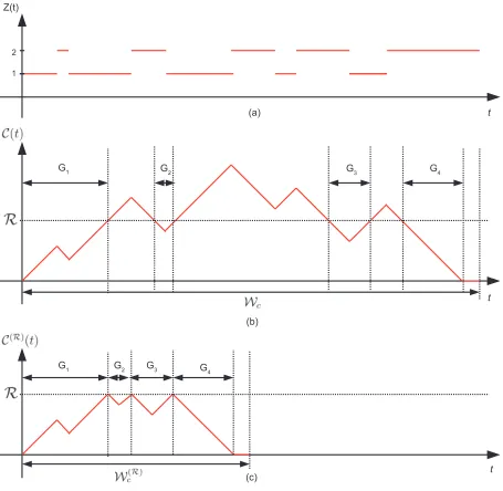
fluid queues in Figure 1.1 (a), (b), and (c) respectively. As observed in the Figures 1.1
(b) and (c), on one hand, once the fluid level {C(t)}t≥0 of the finite fluid queue reaches
level R, the fluid level starts (instantly) to decrease at rate −1. On the other hand, the
fluid level C(t)}t≥0 of the ordinary fluid queue can go beyond level R. Denote by B the
busy period of the driving M/G/1 queue of the finite fluid queue, it is important to note
that P[B ≤ R] = 1 as the consequence of the upper boundary of the fluid level R.
As observed in Figure 1.1, the duration of the time that the fluid level {C(t)}t≥0 of the
1.4. Applications of level crossing methods on fluid queues
Figure 1.1: A sample path of fluid level and driving process of ordinary fluid queue. (a) {Z(t)}t≥0, (b) {C(t)}t≥0, (c) {C(R)(t)}t≥0.
the time that the fluid level {C(R)(t)}t
≥0 of the finite fluid queue is below levelR. Thus,
we have
Z Wc(R)
0
I(0,R) "
{C(R)(t)}t≥0
dt=
Z Wc
0
I(0,R)({C(t)}t≥0)dt, (1.42)
where I(x,y)(•) is an indicator function. The expression in the left-hand side of (1.42)
refers to the duration of time that the sample path of fluid level {C(R)(t)}t
1.4. Applications of level crossing methods on fluid queues
over (0,Wc(R)), and the expression in the right-hand side of (1.42) refers to the duration of time that the sample path of the fluid level {C(t)}t≥0 is below R over (0,Wc). For
instance, as observed in Figure 1.1, both sides of (1.42) equal to G1 +G2 +G3 +G4.
Denote by Wc the complete cycle (the non-empty period + the empty period) of the
ordinary fluid queue. The LST of the Wc is discussed in Section 2.3.3 and the expected
value of the Wc is expressed in (2.18). Denote by Wc(R) the complete cycle (the non-empty period + the non-empty period) of the finite fluid queue. By the Renewal Reward Theorem [34, Section 7.4, Proposition 7.3], the expected complete cycle of the finite fluid queue can be expressed in terms of the proportion of the expected complete cycle of the
ordinary fluid queue, namely
E[Wc(R)] = lim
t→∞P[C(t)≤ R]E[Wc] =P[C ≤ R]E[Wc]. (1.43)
Denote byπE the long-run proportion of time that the fluid level of the finite fluid queue
is at level 0, by the Renewal Reward Theorem ([34, Section 7.4, Popposition 7.3]), we have
πE =
1
λ·P[C ≤ R]·E[Wc], (1.44)
where λ is the arrival rate of the driving M/G/1 queue for the finite fluid queue. Thus,
1/λis the expected empty period of the finite fluid queue. By the Smith’s Theorem [37],
for 0< x <R, the cumulative distribution function of the ordinary fluid queue and finite
fluid queue can be expressed in terms of the long-run proportion of the time that the
fluid level is below levelx, namely
P[C ≤x] =
RWc
0 I(0,R)({C(t)}t≥0)dt
E[Wc]
, (1.45)
P[C(R) ≤x] =
RWc(R)
0 I(0,R) "
{C(R)(t)}t
≥0
dt
E[Wc(R)]
1.4. Applications of level crossing methods on fluid queues
The expressions (1.42), (1.45) and (1.46) suggest that
P[C(R) ≤x] = E[Wc]·P[C ≤ x] E[Wc(R)]
, 0< x <R. (1.47)
Substituting the expression (1.43) into (1.47) yields
P[C(R)≤x] = P[C ≤ x]
P[C ≤ R], 0< x <R. (1.48)
Denote by Ce(s) the LST of the pdf of the fluid level of the ordinary fluid queue, then
the cdf of the C can be computed by taking inverse LST of C(s)/se using Euler and
post-Widder algorithms [1, 2, 3].
1.4.3
Example 3: Distribution of the fluid level in a fluid queue
with an upper barrier
R
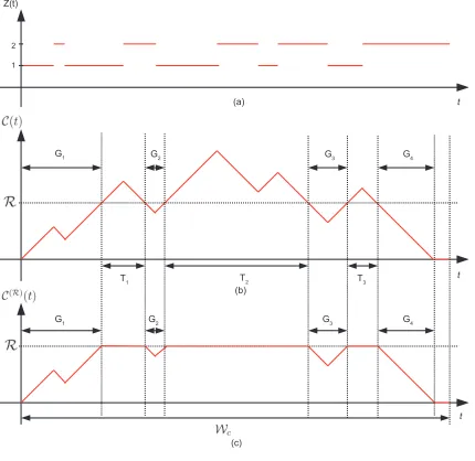
A sample path of the states{Z(t)}t≥0 of the driving M/G/1 queue and a sample path of
the fluid level {C(t)}t≥0 of the fluid queue driven by an M/G/1 queue are illustrated in
Figure 1.2 (a) and (b) below, respectively. As observed, during the busy periods of the
driving queue{Z(t) = 1}t≥0, the fluid level increases at rate 1. During the idle period of
the driving queue {Z(t) = 1}t≥0, the fluid level decreases at rate −1 as long as the fluid
level is above 0. We refer the fluid queue driven by anM/G/1 queue as an ordinary fluid
queue. In this example, we are interested in distribution of the fluid level of a fluid queue
with an upper barrier R, such that whenever the fluid level {C(t)}t≥0 of the ordinary
fluid queue is above level R, the fluid level {C(R)(t)} of the fluid queue with an upper
barrier R stays at level R. The sample path of the fluid level {C(R)}t
≥0 is illustrated in
Figure 1.2 (c) below. Here, we assume that the fluid level {C(R)(t)}t
≥0 of the fluid queue
1.4. Applications of level crossing methods on fluid queues
Figure 1.2: The sample paths of the processes: (a) {Z(t)}t≥0, (b) {C(t)}t≥0, (c)
{C(R)(t)}t
≥0.
Denote by Wc the complete cycle (non-empty fluid period plus empty fluid period) of
the fluid queue driven by an M/G/1 queue discussed in Section 1.2.1. We refer to the
fluid queue driven by an M/G/1 with arrival rate λ and expected service time 1/µ as
ordinary fluid queue. The LST of the pdf of the fluid level C of the ordinary fluid queue
is given in (1.4).
Denote by πR the long-run proportion of time that the fluid level is above level R and
1.4. Applications of level crossing methods on fluid queues
Reward Theorem ([34, Section 7.4, Popposition 7.3]), we have
πR= E
[time aboveR in Wc]
E[Wc] = limt→∞P[C(t)≥ R] =P[C ≥ R], (1.49)
Letting s go to ∞in (1.4) yield
πE =
1−λE[B] 1 +λE[B] =
E[I]
E[Wc], (1.50)
whereB and I are the busy and idle period of the drivingM/G/1 queue of the ordinary
fluid queue respectively. Using the expressions (1.49) and (1.50) yields
P[0<C <R] = 1− E[I] +E[time aboveR in Wc]
E[Wc] =P[C ≤ R]−πE, (1.51)
as expected. As observed in Figure 1.2, the long-run proportion of time forCR in (0,R)
equals to the long-run proportion of time for C in (0,R), thus we have the duration of
the time that the fluid level {C(t)}t≥0 of the ordinary fluid queue below level R (i.e.
G1+G2+G3+G4) equals the duration of the time that the fluid level {C(R)(t)}t≥0 below
R (i.e. G1+G2+G3+G4). Thus, we have
Z Wc
0
I(0,R) "
{C(R)(t)}t≥0
dt=
Z Wc
0
I(0,R)({C(t)}t≥0)dt. (1.52)
Since the expected duration of the complete cycleE[Wc] for the ordinary fluid queue and
fluid queue with upper barrier R is the same, by the Smith’s Theorem [37], we have
P[0<CR <R] =P[0<C <R], 0< x <R. (1.53)
1.5. Conclusion
barrier R is
P[0<CR <R] =P[0<C <R], 0< x <R, (1.54)
with a point mass at level 0 with probability πE =P[C ≤0] and a point mass at level R
with probability πR=P[C ≥ R].
1.5
Conclusion
To summarize this chapter, we introduce an LC method and indicate how to apply it
to derive the pdf of fluid level of the finite and infinite-capacity fluid queue driven by
an M/G/1 queue, and the probability of the busy period of an M/G/1 queue being
Chapter 2
Infinite capacity fluid system
We consider a fluid queue with infinite capacity driven by anM/G/1 queue investigated
by J. Virtamo and I. Norros in [44]. As usual, the fluid content empties at rate r2
continuously as long as the content is non-empty, and the content fills at net rate r1 as
long as the server of the driving queue is busy. The structure of this chapter is as follows:
in Section 2.1, we define the fluid queue driven by an M/G/1 queue, and introduce the
terminologies used in this dissertation. In Section 2.2, we derive the distribution of the
fluid level using thelevel crossing(LC) methods together with atriangle diagram; then we
formulate the probability density function (pdf) of the fluid level in terms of a Beneˇs-like
series [16, 24, 32]. In Section 2.3, we use a probabilistic interpretation of the
Laplace-Stieltjes transform (LST) to interpret the LST of the pdf of the non-empty period of the
fluid queue1 [11, 24, 35]. In Section 2.4, we derive the probability generating functions
(pgf) of the number of thetagged arrivals, thearrivals served, and thethe number of peaks
in a non-empty period of the fluid queue. In Section 2.5, a simulation of the expected
values of fluid level and non-empty period is conducted and the simulated results are then
compared to the theoretical results. Lastly, we provide two examples to demonstrate the
2.1. Fluid queue driven by an M/G/1 queue
connection between the fluid queue and the M/G/1 queue with multiple inputs and the
M/G/1 queue with a balking discipline, in Section 2.6.
2.1
Fluid queue driven by an
M/G/
1
queue
2.1.1
Introduction
Denote by {C(t)}t≥0 the fluid level at time t, and by {Z(t)}t≥0 the Markov renewal
process at time t which takes values in the finite state space Ω := {1,2, . . . , n}. We
refer to the two-dimensional Markov process {C(t), Z(t)}t≥0 as a fluid queue driven by
a Markov renewal process (or more formally, an environmental process) {Z(t)}t≥0. The
rates at which the fluid content of the fluid queue fills and empties are governed by the
process {Z(t)}t≥0 in such a way that
dC(t)
dt =
rZ(t), C(t)>0,
max(0, rZ(t)), C(t) = 0,
(2.1)
where rZ(t) ∈ R is a rate corresponding to the sojourn of Z(t) = i. In this chapter, we
assume that the Markov renewal process {Z(t)}t≥0 is an M/G/1 queue status, which
takes values in the finite state space Ω ={1,2} such that
Z(t) =
1, if the server of the M/G/1 queue is busy,
2, if the server of the M/G/1 queue is idle,
(2.2)
with the net input rater1 >0 and continuous leaking rate r2 <0.
To recap the characteristics of the fluid queue driven by an M/G/1 queue (henceforth
2.1. Fluid queue driven by an M/G/1 queue
continuously as long as the content is non-empty, and the content fills at net rate r1 as
long as the server of the driving M/G/1 queue is busy.
2.1.2
Terminology of the fluid queue
We define
φ(t) =
0, if C′(t) = 0 and Z(t) = 2,
1, if C′(t)>0 and Z(t) = 1,
2, if C′(t)<0 and Z(t) = 2,
(2.3)
where C′(t) := dC(t)/dt, as the states of the fluid process {C(t), Z(t)}
t≥0 at time t. We
refer to (1) the state {φ(t) = 0}t≥0 as an empty period with notationE; (2) the state
{φ(t) = 1}t≥0 as an activity period with notation A; (3) the state {φ(t) = 2}t≥0 as a
silence period with notationS. These terminologies have been used in the fluid queue
literature [9, 10, 20, 21, 26]. For each complete cycle (non-empty period plus empty
period) of the fluid queue, denote byAT theduration of activity periods, and byST
the duration of silence periods in a complete cycle of the fluid queue respectively.
Finally, denote by Wc := AT +ST +E the wet cycle (complete cycle) of the fluid
queue, and by W := AT +ST the wet period (non-empty period) of the fluid queue.
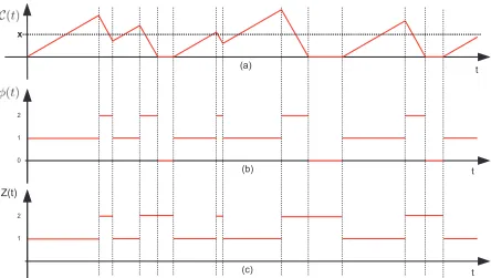
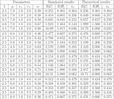
A typical sample path of the fluid level {C(t)}t≥0, the states of the fluid queue {φ(t)}t≥0
and the states of the driving M/G/1 queue {Z(t)}t≥0 corresponding to the fluid queue
are illustrated in Figure 2.1.
Remark 2.1.1. As observed in Figure 2.1 and using the expressions (2.2) - (2.3), we have
{φ(t) = 1}t≥0 = {Z(t) = 1}t≥0, and {φ(t) = 0}t≥0 S {φ(t) = 2}t≥0 = {Z(t) = 2}t≥0.
2.1. Fluid queue driven by an M/G/1 queue
Figure 2.1: (a) A typical sample path of fluid level. (b) The states of the fluid queue. (c) The states of the driving M/G/1 queue.
2.1.3
Definition of the probability density function of the fluid
level
In this section, we define a partial probability density function (ppdf) and a total (or
marginal) pdf of the fluid level. For x > 0, define the steady-state partial cumulative
probability distribution function (cdf) of the fluid level as
Fi(x) := lim
t→∞P[0<C(t)≤x, φ(t) =i] + limt→∞P[φ(t) = 0], i= 1, 2, (2.4)
where φ(t) is defined in (2.3). The steady-state partial pdf is defined as
fi(x) =
d dx
lim
t→∞P[C(t)≤x, φ(t) =i]
2.1. Fluid queue driven by an M/G/1 queue
Define the total pdf of the fluid level as
f(x) = d dx
lim
t→∞P[C(t)≤x]
, x >0. (2.6)
The total pdf of the fluid level is
f(x) = f1(x) +f2(x), x >0. (2.7)
We remark that the partial pdff1(x) corresponds to the fluid level in the activity period,
and the partial pdf f2(x) corresponds to the fluid level in the silence period. More
importantly, the expression (2.4) indicates that there has a point mass for the distribution
of the fluid level at 0. Finally, it is important to highlight that
Z ∞
0
f1(x)dx6= 1 and
Z ∞
0
f2(x)dx6= 1. (2.8)
2.1.4
Stability condition of the fluid queue
For a fixedx >0 andt >0, defineUt(x) and Dt(x) be the number of up- and
downcross-ings of levelxduring the time interval (0, t) respectively. Brill [12, Section 6.2.7, pp. 304
- 309] shows that the up- and downcrossing rate of level x during the time interval (0, t)
are
lim
t→ ∞
Ut(x)
t
a.s.
= r1f1(x) and lim t→ ∞
Dt(x)
t
a.s.
= r2f2(x), x >0, (2.9)
where f1(x) and f2(x) are defined in (2.5) respectively. Here r1 and r2 are the net
input rate and the continuous leaking rate of the fluid queue respectively. Let πE :=
lim
t→∞P[φ(t) = 0] be the point mass of the fluid level at 0. Using a LC argument, the rate
2.1. Fluid queue driven by an M/G/1 queue
by (2.9), we have r1f1(0+) = λπE = r2f2(0+). The term λπE is the rate at which an
arrival arrives to the empty M/G/1 queue while the fluid content is also empty, and
this particular arrival initiates a busy period in the driving M/G/1 queue and causes
the sample path to leave level 0. Each time point when {C(t)}t≥0 leaves level 0 is a
regenerative point [36, 43]. Hence, {C(t)}t≥0 is a regenerative process with wet cycle Wc
that forms a renewal process. By theElementary Renewal Theorem [34, Section 7.3, pp. 407 - 416], E[Wc] = 1/(λπE). By the Renewal Reward Theorem [34, Proposition 7.3, pp.
416 - 417], the long-run proportion of time that {φ(t) = 1 or 2}t≥0 is
E[{φ(t) = 1 or 2}t≥0]
E[{φ(t) = 0}t≥0] +E[{φ(t) = 1 or 2}t≥0]
= E[W] E[Wc]
= 1−πE. (2.10)
For each wet cycle, the amount of fluid entering equals the amount of fluid leaving the
fluid content. Consequently, we have
r1 lim
t→∞P[{φ(t) = 1}t≥0] =r2t→∞lim P[{φ(t) = 2}t≥0]. (2.11)
The expression (2.11) leads to
r1AT =r2ST, (2.12)
given that E[Wc]<∞. In addition, by the Remark 2.1.1, we have ∀t >0,P[φ(t) = 1] =
P[Z(t) = 1], i.e., A and B are identical distributed, where B is the busy period of the
driving M/G/1 queue. Since each wet cycle consists multiple of busy cycles (Np) of the
driving M/G/1 queue, and E[AT] = E[Np]·E[A] = E[Np]·E[B], we have the long-run
proportion of the time of theAT equals the traffic intensity of the driving M/G/1 queue,
namely: ρ := λ/µ := (E[Np]·E[B])/(E[Np]·(E[B] +E[I])), where I is the idle period
2.1. Fluid queue driven by an M/G/1 queue
this property with (2.10) and (2.11), we obtain
πE = 1−
1 + r1 r2
ρ= 1−
1 + r1 r2
E[B] E[B] +E[I]
. (2.13)
Setting 0< πE ≤1 yields the stability condition of the fluid queue, namely
r2E[I]> r1E[B]. (2.14)
If this condition is not satisfied, then the steady-state distribution of the fluid level does
not exist. Considering that the activity periods of the fluid queue are governed by the
busy periods of theM/G/1 queue, the stability condition (2.14) states that the expected
(net) fluid entering the fluid content during the busy period of the M/G/1 queue has to be less than the expected fluid leaving the fluid content during the idle period of the
M/G/1 queue.
2.1.5
Expected values of the fluid queue
Denote by Np the number of complete busy cycles of the M/G/1 queue in a wet cycle.
Figure 2.2 illustrates the composition of a wet cycle of the fluid queue in terms of activity
and silence periods, and empty periods.
On one hand, the expected wet cycle can be written as
E[Wc] =E
"XNp
i=1
(Bi+Ii)
#
=E[Np] (E[B] +E[I]). (2.15)
On the other hand, since the arrival process of the driving M/G/1 queue is a Poisson
2.2. Fluid queue driven by an M/G/1 queue
as
E[Wc] =E[AT] +E[ST] +E[E] =
1 + r1 r2
E[Np]E[B] +E[I], (2.16)
where E[E] =E[I], and AT,ST,and E are defined in Section 2.1.1.
Figure 2.2: Composition of a single wet cycle
Equating (2.15) and (2.16), and collecting the terms yield
E[Np] = E
[I] E[I]− r1
r2E[B]
. (2.17)
The expression (2.17) implies, by (2.12) and (2.16), that
E[AT] = E
[I]E[B] E[I]−r1
r2E[B]
and E[W] = E[B](E[I])
2
E[I]− r1
r2E[B]
. (2.18)
As observed in Figure 2.2, it is important to highlight that Np can be also interpreted as
2.2. Probability distribution of the fluid level
2.2
Probability distribution of the fluid level
2.2.1
Downcrossing and upcrossing rates of level
x
Recall that, for x > 0 and t > 0, the upcrossing and downcrossing rates at which the
sample path of the fluid level crosses level xfrom above and below are given in (2.9). In
addition, the rate at which the sample path of the fluid level upcrosses level x can be
expressed as2
r1f1(x) =λπEB
x r1
+λ
Z y=x
y=0+
B
x−y r1
f2(y)dy, (2.19)
where B(•) is the complementary cumulative distribution function (ccdf) of the busy
period of the driving M/G/1 queue. In addition, since the upcrossing rate of level x
equals the downcrossing rate, the expression (2.19) can be interpreted as the downcrossing
rate of level x (i.e., r2f2(x)) as well. The first term on the right hand side of (2.19) is
the rate at which the sample path upcrosses level x starting at level 0, and the second
term of the right hand side of (2.19) is the rate at which the sample path upcrosses level
of x starting from level y in the interval (0, x). For details, readers are referred to [12,
Section 1.6 and 1.7, pp. 13 - 17].
Observation 2.2.1. Letting r1 =r2 = 1 in (2.19) yields a LC equation analogous to the
equation for the pdf of the virtual waiting time for an M/G/1 queue (see [12, p. 17] for the details). It hints that the LC equation of the fluid level links to the LC equation of the virtual waiting time of an M/G/1 queue with adjustment for the rates. However, it is important to point out that πE is the point mass at level 0 for the fluid level instead of
the point mass of the virtual waiting time at level 0 for an M/G/1 queue.
2r
2.2. Probability distribution of the fluid level
2.2.2
Triangle diagram
In this section, we introduce a triangle diagram for the sample path of the fluid level which can be applied to express the upcrossing rate r1f1(x) and the downcrossing rate
r2f2(x) in terms of the pdf of the fluid levelf(x).
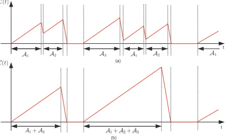
Figure 2.3: (a) A typical sample path of fluid level. (b) A corresponding sample path of fluid level.
Figure 2.3 illustrates the sample paths of the fluid level. In Figure 2.3, both sample
paths encompass two complete wet cycles and one incomplete wet cycle. Specifically, in
Figure 2.3 (a), the first wet cycle encompasses two activity and silence periods, and the
second wet cycle encompasses three activity and silence periods. In Figure 2.3 (b), both
wet cycles encompass one activity and one silence periods. Although, the fluid level at
time t in Figure 2.3 (a) and (b) are different in general, the duration of the activity AT
2.2. Probability distribution of the fluid level
activity and silence periods in a wet cycle do not affect the duration of activity and silence
periods; or the duration of wet period. Thus, if we would like to expressf1(x) andf2(x) in
terms off(x), then the information achieved from 2.3 (b) are identical to the information
achieved from 2.3 (a). Hence, to simplify our work, in this section, we focus on Figure 2.3
(b). It is important to point out here that the processes demonstrated in Figure 2.3 (a)
and (b) are both regenerative processes. Thus by the theory of regenerative processes, for
these particular figures, the long-run proportion of time of the activity periods achieved
using the first wet cycle equals the long-run proportion of time of the activity periods
achieved using the second wet cycle. Thus, we will express f1(x) and f2(x) in terms of
f(x) using the first wet period, and refer to the diagram of as a triangle diagram. Figure 2.4 illustrates the triangle diagram of the fluid level in a wet cycle.
Figure 2.4: Triangle diagram of the fluid level
Denote byAT =A1+A2+A3 the duration of the activity periods in the first wet cycle in
Figure 2.4; then the duration of the silence periods is (r1AT)/r2. Thus, the proportions
of time of the activity and silence periods are
r2
r1+r2
and r1
r1 +r2
2.2. Probability distribution of the fluid level
respectively. The above expression implies that the weights associated with f(x) on
{φ(t) = 1}t≥0 and {φ(t) = 2}t≥0 are r2/(r1 +r2) and r1/(r1 +r2) respectively. These
properties suggest that (x >0)
f1(x) =
r2
r1+r2
f(x) and f2(x) =
r1
r1 +r2
f(x). (2.21)
The expression (2.21) does not violate the principle of rate balance condition (see [12, p.
16] for the details) at which the necessary condition for (2.21) to be true is
lim
t→∞
Dt(x)
t =r1f1(x) = r1r2
r1+r2
f(x) =r2f2(x) =
r1r2
r1+r2
f(x) = lim
t→∞
Ut(x)
t (2.22)
(i.e., the downcrossing rate of level x equals the upcrossing rate of level x.) Finally, it
is important to highlight that solving a system of linear equations (i.e., (2.7) and (2.22)
together) gives the same conclusion as shown in (2.21). The intention in this section is
to provide an alternative way to express the rate at which the sample path upcrosses
and downcrosses level x in terms of the pdf of the fluid level as well as visualizing the
concepts behind the mathematics.
We end this section by highlighting the limitations of thetriangle diagram when applied to express f1(x) andf2(x) in terms of f(x). Thetriangle diagram approach discussed in
this section relies on the two assumptions: (1) thenet input andcontinuous leaking rate are constant, and (2) the wet cycle is a regenerative process.
2.2.3
Level-crossing equations
Substituting (2.21) into (2.19) yields an LC equation for the pdf of the fluid level, namely
r1r2
r1+r2
f(x) = λπEB
x r1 +λ r1
r1+r2
Z y=x
y=0+
B
x−y r1
2.2. Probability distribution of the fluid level
Remark 2.2.2. The expression (2.23) can be interpreted in two ways: (1) equating two different expressions of the upcrossing rate at level x. (2) balancing upcrossing and downcrossing rates of level x, since r1f1(x) =r2f2(x).
2.2.4
Beneˇ
s-like series for PDF of fluid level
In this section, we formulate the pdf of the fluid level using a LC argument (see [13] for
more details) which explains the meaning of Beneˇs’ mathematical series first introduced
by Beneˇs in [6] for the pdf of the virtual waiting time of an M/G/1 queue (discussed
and made noteworthy by Kleinrock [24]). Two completely different explanations of the
Beneˇs’ series for the pdf of the virtual waiting time of an M/G/1 queue are given by
Cooper and Niu in [16] and Prabhu in [32].
Consider the equation (2.23). Applying a technique similar to that in Brill [13], we
multiply by r1+r2 and divide by r1r2 to yield
f(x) = λπE
1 r1 + 1 r2 B x r1 + λ r2 Z y=x y=0+ B
x−y r1
f(y)dy, x >0. (2.24)
We divide and multiply byE[B] in the first term of the right-hand side of above equation
to yield
λE[B]πE
1 r1 + 1 r2 1 E[B]B
x r1
=ρBπE
1 r1 + 1 r2 g∗1 x r1
, x >0, (2.25)
whereρB =λE[B] and g∗k(x/r1) is thek-fold self convolution of the residual time of the
busy period at x/r1 of the driving M/G/1 queue, k = 1,2, . . .. Next, we substitute the
2.2. Probability distribution of the fluid level
This gives (for x >0)
λ r2 Z y=x y=0 B
x−y r1 f(y)dy = λ r2 Z y=x y=0 B
x−y r1 λπE 1 r1 + 1 r2 B y r1 dy + λ r2 Z y=x y=0 B
x−y r1 λ r2 Z z=y z=0 B
y−z r1 f(z)dz dy = λ 2 r2 πE 1 r1 + 1 r2 Z y=x y=0 B
x−y r1 B y r1 dy + λ r2
2Z y=x
y=0
Z z=y
z=0
B
x−y r1
B
y−z r1
f(z)dzdy. (2.26)
In the second-last term of (2.26), multiplying and dividing (E[B])2 yields
λ2 r2 πE 1 r1 + 1 r2 Z y=x y=0 B
x−y r1 B y r1 dy = ρ 2 B r2 πE 1 r1 + 1 r2 Z y=x y=0 1 E[B]B
x−y r1
1 E[B]B
y r1
dy. (2.27)
Notice that the integral from equation (2.27) can be further simplified to
Z y=x
y=0
1 E[B]B
x−y r1
1 E[B]B
y r1
dy =r1
Z u=x/r1
u=0
1 E[B]B
x r1 −u 1
E[B]B(u)du
=r1g∗2
x r1
. (2.28)
Thus equation (2.27) can be further simplified to
λ2 r2 πE 1 r1 + 1 r2 Z y=x y=0 B
x−y r1 B y r1 dy
= r1 r2
ρ2BπE
1 r1 + 1 r2 g∗2 x r1
=πE
r1+r2
r2 1 r1 r2 ρB 2 g∗2 x r1 . (2.29)
2.2. Probability distribution of the fluid level
yields (for x >0)
λ r2
2Z y=x
y=0
Z z=y
z=0
B
x−y r1
B
y−z r1 f(z)dzdy = λ r2
2Z y=x
y=0
Z z=y
z=0
B
x−y r1
B
y−z r1 λπE 1 r1 + 1 r2 B z r1
dzdy+. . .
= λ3 r2 2 πE 1 r1 + 1 r2 Z y=x y=0 Z z=y z=0 B
x−y r1
B
y−z r1 B z r1
dzdy+. . . .
Multiplying and dividing by (E[B])3 in the above equation yields
λ r2
2Z y=x
y=0
Z z=y
z=0
B
x−y r1
B
y−z r1
f(z)dzdy
=πE
r1+r2
r2 1 r1 r2 ρB 3
g∗3
x r1
+. . . . (2.30)
Repeatedly substituting for f(•), we get
f(x) =
πE, x= 0,
πE
r1+r2
r2 1 X∞ k=1 r1 r2 ρB k g∗k x r1
, x > 0. (2.31)
The expression (2.31) suggests that for x > 0, f(x) is the weighted sum of convolved
residual busy periods of B ar x/r1. Integrating (2.31) with respect to x over (0+,∞)
yields
Z x=∞
x=0+
f(x)dx=
Z x=∞
x=0+
πE
r1+r2
r2 1 X∞ k=1 r1 r2 ρB k g∗k x r1 dx
=πE
r1 +r2
r1 ∞ X k=1 r1 r2 ρB k . (2.32)
Using the normalization condition,
πE +
Z x=∞
x=0+
2.3. Laplace-Stieltjes transform
and (2.32) gives
πE = 1 +
r1 +r2
r1
X∞
k=1
r1
r2
ρB
k!−1
= 1 +
r1 +r2
r1
r1
r2
λE[B] 1
1−r1
r2λE[B]
!−1
= r2−r1λE[B] r2+r2λE[B]
(2.34)
where we assume that the geometric series in equation (2.32) converges to a number.
Letting 0< πE <1, we obtain
r1
r2
ρB <1 ⇐⇒ r1E[B]< r2E[I] (2.35)
which is the stability condition of the fluid queue in (2.14). Finally, since B is the busy
period of the driving M/G/1 queue with arrival rate λ and expected service time 1/µ,
substituting E[B] = 1/(µ−λ) into (2.34) gives (2.13).
2.3
Laplace-Stieltjes transform
2.3.1
Introduction
Denote by X the random variable that has a legitimate probability density function
f(x), x≥0. The Laplace-Stieltjes transform (LST) off(x) named after the
mathemati-cian Pierre Simon Laplace, is defined as
Lf(s) =
Z ∞
0−