Numerical Simulation of Wind Load on Roof Mounted Solar Panels

(1)

University of Windsor University of Windsor

Scholarship at UWindsor

Electronic Theses and Dissertations Theses, Dissertations, and Major Papers

2012

Numerical Simulation of Wind Load on Roof Mounted Solar

Panels

Yuanming Yu University of Windsor

Follow this and additional works at: https://scholar.uwindsor.ca/etd

Recommended Citation Recommended Citation

Yu, Yuanming, "Numerical Simulation of Wind Load on Roof Mounted Solar Panels" (2012). Electronic Theses and Dissertations. 218.

https://scholar.uwindsor.ca/etd/218

This online database contains the full-text of PhD dissertations and Masters’ theses of University of Windsor students from 1954 forward. These documents are made available for personal study and research purposes only, in accordance with the Canadian Copyright Act and the Creative Commons license—CC BY-NC-ND (Attribution, Non-Commercial, No Derivative Works). Under this license, works must always be attributed to the copyright holder (original author), cannot be used for any commercial purposes, and may not be altered. Any other use would require the permission of the copyright holder. Students may inquire about withdrawing their dissertation and/or thesis from this database. For additional inquiries, please contact the repository administrator via email

(2)

i

Numerical Simulation of Wind Load on Roof Mounted Solar Panels

by

Yuanming Yu

A Thesis

Submitted to the Faculty of Graduate Studies through the Department of Mechanical,

Automotive and Materials Engineering in Partial Fulfillment of the Requirements for the

Degree of Master of Applied Science at the University of Windsor

Windsor, Ontario, Canada

2012

(3)

ii

Numerical Simulation of Wind Load on Roof Mounted Solar Panels

by

Yuanming Yu

Approved By:

Dr. Shaohong Cheng, External Department Reader

Department of Civil and Environmental Engineering

Dr. David Ting, Department Reader

Department of Mechanical, Automotive and Materials Engineering

Dr. Ronald Barron, Co-Advisor

Department of Mathematics and Statistics and Department of Mechanical,

Automotive and Materials Engineering

Dr. Ram Balachandar, Co-Advisor

Department of Civil and Environmental Engineering and Department of Mechanical,

Automotive and Materials Engineering

Dr. N. Zamani, Committee Chair

(4)

iii

AUTHOR’S DECLARATION OF ORIGINALITY

I hereby certify that I am the sole author of this thesis and that no part of this

thesis has been published or submitted for publication.

I certify that, to the best of my knowledge, my thesis does not infringe upon

anyone’s copyright nor violate any proprietary rights and that any ideas, techniques,

quotations, or any other material from the work of other people included in my thesis,

published or otherwise, are fully acknowledged in accordance with the standard

referencing practices. Furthermore, to the extent that I have included copyrighted material

that surpasses the bounds of fair dealing within the meaning of the Canada Copyright

Act, I certify that I have obtained a written permission from the copyright owner(s) to

include such material(s) in my thesis and have included copies of such copyright

clearances to my appendix.

I declare that this is a true copy of my thesis, including any final revisions, as

approved by my thesis committee and the Graduate Studies office, and that this thesis has

(5)

iv

ACKNOWLEDGEMENTS

I would never have been able to finish my thesis without the guidance of my

committee members, help from my colleagues, and supports from my family and wife.

Dr. Ting and Dr. Cheng presented a lot of interesting questions in the proposal

meeting, which pushed me to think deeper and wider. Many colleagues, especially Kohei,

gave me much help during my research period. I really appreciate their kind help.

I would like to take this opportunity to express my deepest gratitude to my

advisors, Dr. Barron and Dr. Balachandar for their great guidance, caring, patience and

providing me with an excellent research atmosphere. I also really want to thank the

Natural Sciences and Engineering Research Council (NSERC) and Polar Racking Inc. for

providing an NSERC Industrial Postgraduate Scholarship to carry out my research. I also

offer my thanks to the University of Windsor for providing me with Graduate

(6)

v

ABSTRACT

Seven RANS models (Spalart-Allmaras, k-ε, k-ω and their variants, Reynolds Stress Model (RSM)), DES-SST and LES model have been used to predict the pressure

coefficient (Cp) distribution on a cube and the Cp difference of a canopy in an

atmospheric boundary layer flow. The simulation results show that k-ω-SST gives the best prediction in both cases. The RSM also accurately predicts the Cp in the cube case.

The k-ω-SST and DES-SST models have been used to simulate the wind load on flat roof mounted solar panels under similar flow conditions with different wind attack angles. The

simulation results demonstrate that both k-ω-SST and DES-SST give good prediction of the drag force at all wind attack angles and reasonably good prediction of the lift force at

(7)

vi

LIST OF TABLES

Table 2.1 Extent of computational domain (h: cube height)………....10

(12)

xi

LIST OF FIGURES

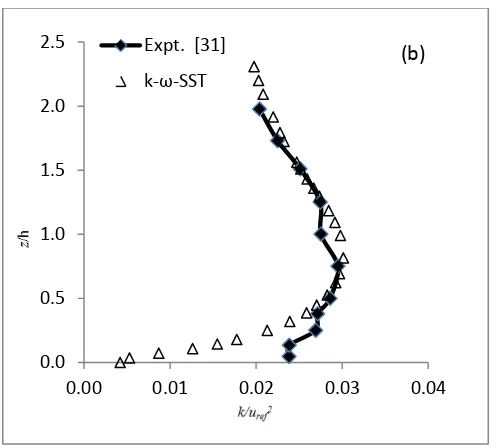
Fig. 2-1 Comparison of experimental results and numerical prediction (k-ω-SST) at cube

location, without presence of the cube, (a) velocity profile; (b) turbulent kinetic energy...7

Fig. 2-2 Computational domain II (horizontal layout, not to scale)………..…11

Fig. 2.3 Computational domain II (cross-sectional layout, not to scale)………...…11

Fig.2-4 Effect of computational domain size on Cp distribution………...…12

Fig 2-5 Tetrahedral mesh around the cube………13

Fig. 2-6 Cp distribution at vertical symmetry plane from (a) k-ω standard and k-ω-SST models; (b) Reynolds Stress Model (RSM) and Spalart-Allmaras (SA) model………....16

Fig. 2-7 Cp distribution at vertical symmetry plane from (a) k-ε standard, k-ε RNG and k-ε Realizable models; (b) DES–SST and LES (dynamic Smagorinsky) models………...17

Fig. 2-8 Streamtraces predicted by Spalart-Allmaras model, (a) vertical symmetry plane; (b) horizontal plane at 0.125h……….….…..18

Fig. 2-9 Streamtraces predicted by k-ε standard model, (a) vertical symmetry plane; (b) horizontal plane at 0.125h……….…….…..19

Fig. 2-10 Streamtraces predicted by k-ε RNG model, (a) vertical symmetry plane; (b) horizontal plane at 0.125h………...19

Fig. 2-11 Streamtraces predicted by k-ε Realizable model, (a) vertical symmetry plane; (b) horizontal plane at 0.125h……….………...20

Fig. 2-12 Streamtraces predicted by k-ω standard model, (a) vertical symmetry plane; (b) horizontal plane at 0.125h……….…...20

Fig. 2-13 Streamtraces predicted by k-ω-SST model, (a) vertical symmetry plane; (b) horizontal plane at 0.125h……….………...21

(13)

xii

Fig. 2-15 Streamtraces predicted by DES-SST model, (a) vertical symmetry plane; (b)

horizontal plane at 0.125h……….….…...22

Fig. 2-16 Streamtraces predicted by LES (dynamic Smagorinsky), (a) vertical symmetry

plane; (b) horizontal plane at 0.125h………...…….….…....22

Fig. 3-1 Geometry of the canopy with 0o wind attack angle……….…....26

Fig. 3-2 Velocity profile near canopy location………...…...26

Fig. 3-3 Turbulence intensity profile in streamwise direction near canopy location…....26

Fig. 3-4 Computational domain (horizontal layout, not to scale)………..27

Fig. 3-5 Tetrahedral mesh around the canopy in cross-section layout………...…...28

Fig. 3-6 ∆Cp at different wind attack angles predicted by RANS models (coarse mesh

near the canopy)………..………....…...30

Fig. 3-7 ∆Cp at different wind attack angles by RANS models (fine mesh near the canopy)

………..……….…….…....31

Fig. 3-8 ∆Cp at different wind attack angles by RSM, k-ε standard, RNG, Realizable

(coarse mesh near the canopy)………...…….….….…...32

Fig. 3-9 ∆Cp at different wind attack angles by RSM, k-ε standard, RNG, Realizable (fine

mesh near the canopy)……….………….….…....33

Fig. 3-10 ∆Cp at different wind attack angles by DES-SST and LES (coarse mesh near the

canopy)……….……….…….…..….34

Fig. 3-11 Mean drag coefficient at different wind attack angles by DES-SST and LES

(coarse mesh near the canopy)………...…....35

Fig. 3-12 Mean lift coefficient at different wind attack angles by DES-SST and LES

(coarse mesh near the canopy)……….………..…....35

Fig. 3-13 Peak drag coefficient at different wind attack angles by DES-SST and LES

(14)

xiii

Fig. 3-14 Peak lift coefficient at different wind attack angles by DES-SST and LES

(coarse mesh near the canopy)……….……….….…36

Fig. 3-15 Flow velocity vectors near the canopy at wind attack angle of 0o, predicted by k-ω-SST………..….………..…37

Fig. 3-16 Pressure coefficient contours for top of plate e (left) and plate b (right)……...38

Fig. 3-17 Pressure coefficient contours for bottom of plate e (left) and plate b (right)….39 Fig. 4-1 Simulated solar panel layout on a square roof……….41

Fig. 4-2 Velocity profile at location of the building, without presence of the building....42

Fig. 4-3 Turbulence intensity in streamwise direction at building location, without presence of the building………...42

Fig. 4-4 Computational domain horizontal plan layout (not to scale)………...43

Fig. 4-5 Computational domain vertical plan layout (not to scale)………...44

Fig. 4-6 Vertical cross-sectional view of the fine mesh (2mm) around the corner solar panel array………..….…..44

Fig. 4-7 Cp difference on the solar panel predicted by k-ω-SST………..….46

Fig. 4-8 Velocity vectors near the solar panels at 360o wind attack angle………47

Fig. 4-9 Velocity vectors near the solar panels at 320o wind attack angle………47

Fig. 4-10 Velocity vectors near the solar panels at 270o wind attack angle………..48

Fig. 4-11 Velocity vectors near the solar panels at 180o wind attack angle………..48

Fig. 4-12 Cp difference on the wind deflector predicted by k-ω-SST……….…...49

Fig. 4-13 Drag coefficient for the solar panel assembly predicted by k-ω-SST……..…..50

(15)

xiv

Fig. 4-15 Mean drag coefficient for the solar panel assembly predicted by DES-SST (with

coarse mesh)………....…..52

Fig. 4-16 Mean lift coefficient for the solar panel assembly predicted by DES (with

coarse mesh)………..53

Fig. 4-17 Peak drag coefficient for the solar panel assembly predicted by DES (with

coarse mesh)……….…..….…..54

Fig. 4-18 Peak lift coefficient for the solar panel assembly predicted by DES (with coarse

mesh)………..…...54

Fig. 5-1 Drag coefficient for three configurations of the solar panel assembly…..….….57

Fig. 5-2 Velocity vector field at wind attack angle of 330o for vertical spacing of 6 inches

off the roof………..…...58

Fig. 5-3 Velocity vector field at wind attack angle of 330o for vertical spacing at same

height as the parapet………..….…..….58

Fig. 5-4 Lift coefficient for three configurations of the solar panel assembly……….….60

Fig. 5-5 Velocity vectors at wind attack angle of 210o for vertical spacing at the same

(16)

xv

NOMENCLATURE

𝐶𝜇 Constant, used to calculate dynamic turbulent viscosity

∆𝐶𝑝 Pressure coefficient difference

CD Mean drag coefficient

CL Mean lift coefficient

h Height of the cube or building

k Turbulent kinetic energy

kp Turbulent kinetic energy at node P

𝑙 The length scale of flow structure 𝑝 Static pressure

𝑝0 Reference pressure at ambient region

𝑝𝑇 Area averaged pressure at top surface

𝑝𝐵 Area averaged pressure at bottom surface

𝑇𝑖 Turbulent intensity

U Velocity magnitude

𝑈𝑝 Mean velocity in the near wall node P

𝑈∗ _{Nondimensional velocity}

uref Reference velocity in streamwise direction

𝑢𝑖 Velocity components, where i = 1, 2, 3 indicates x, y, z directions

𝑢𝑧 Streamline velocity (x direction) at z coordinate location

𝑢_𝑖′_{Velocity fluctuation, where}_i_{= 1, 2, 3 indicates x, y, z directions}

𝑥𝑖 Coordinates, where i = 1, 2, 3 indicates x, y, z directions

𝑦∗ _{Nondimensional distance from wall}

(17)

xvi

𝑦+ _{Nondimensional distance}

z z coordinate

𝑧𝑟𝑒𝑓 Reference height

𝛼 Exponent of power law or wind attack angle

𝛿𝑖𝑗 Kronecker delta (𝛿𝑖𝑗 = 1 𝑖𝑓𝑖=𝑗𝑎𝑛𝑑𝛿𝑖𝑗 = 0 𝑖𝑓𝑖 ≠ 𝑗)

𝜏𝑖𝑗 Reynolds stress tensor

𝜏𝑤 Wall shear stress

𝜌 Density of the fluid

𝜇 Dynamic viscosity of fluid 𝜇𝑡 Turbulent viscosity of the fluid

𝑣� Modified kinematic viscosity (Spalart-Allmaras)

𝜎𝑣� Constant = 2/3 (Spalart-Allmaras)

𝐶𝑏1 Constant = 0.1355 (Spalart-Allmaras)

𝐶𝑏2 Constant = 0.622 (Spalart-Allmaras)

𝐶𝑣1 Constant = 7.1 (Spalart-Allmaras)

Cw1 Constant for dissipation term (Spalart-Allmaras)

𝑓w Wall damping function, used in dissipation term (Spalart-Allmaras)

Ω� Component of the production term (Spalart-Allmaras)

Ω Magnitude of the vorticity (Spalart-Allmaras) Ω𝑖𝑗 Rate-of-rotation tensor (Spalart-Allmaras)

𝑓𝑣1 Viscosity damping function, used to calculate 𝜇𝑡 (Spalart-Allmaras)

𝑓𝑣2 Wall damping function, used to calculate Ω� (Spalart-Allmaras)

𝛿𝑖𝑗 Kronecker delta (Spalart-Allmaras)

(18)

xvii

𝜒 Ratio of modified kinematic viscosity to viscosity (Spalart-Allmaras)

𝐺𝑘 Production term of k equation (k-ε standard, RNG, Realizable, k-ω standard)

𝑌𝑘 Dissipation term of k equation (k-ε standard)

ε Turbulent energy dissipation rate per unit mass (k-ε)

𝐺𝜀 Production term of ε equation (k-ε standard)

𝑌𝜀 Dissipation term of ε equation (k-ε standard)

𝜎𝑘 Constant = 1.0, used in diffusion term in k equation (k-ε standard)

𝜎𝜀 Constant = 1.3, used in diffusion term in ε equation (k-ε standard)

S Modulus of mean rate-of-strain tensor (k-ε standard) 𝑆𝑖𝑗 Strain tensor (k-ε standard)

𝐶1𝜀 Constant, used in production term in ε equation (k-ε standard)

𝐶2𝜀 Constant, used in dissipation term in ε equation (k-ε standard)

𝛼𝑘 Constant = 1.39, used for diffusion term in equation of k (RNG)

𝜇𝑒𝑓𝑓 Effective viscosity (RNG)

𝛼𝜀 Constant = 1.39, used for diffusion term in equation of ε (RNG)

𝐶1𝜀 Constant for production term in equation of ε (RNG)

𝐶2𝜀∗ Constant for dissipation term in equation of ε (RNG)

𝐶2𝜀 Constant, used to find 𝐶2𝜀∗ (RNG)

𝐶𝜇 Constant = 0.0845, used in turbulent viscosity (RNG)

𝜂 Constant obtained from modulus of mean rate-of-strain tensor (RNG)

𝜂0 Constant = 4.377, used to find 𝐶2𝜀∗ (RNG)

𝛽 Constant = 0.012, used to find 𝐶_2𝜀∗ (RNG) 𝐶𝜇 Constant for turbulent viscosity (Realizable)

𝑈∗ _{Constant, used to calculate}_𝐶

(19)

xviii

Ω𝑖𝑗 Mean rate-of-rotation tensor (Realizable)

ωk Angular velocity (Realizable)

𝜀𝑖𝑗𝑘 Permutation tensor (Realizable)

A0 Model constant = 4.04, used to find value of 𝐶𝜇 (Realizable)

𝐴𝑠 Model variable constant, used to find value of 𝐶𝜇 (Realizable)

𝐶1 Constant, used in production term of 𝜀 equation (Realizable)

𝐶2 Constant = 1.9, used in dissipation term of 𝜀 equation (Realizable)

𝜎𝑘 Constant = 1.0, used in diffusion term of k equation, (Realizable)

𝜎𝜀 Constant = 1.2, used in diffusion term of ε equation (Realizable)

𝜙 Constant angle, used to find 𝐴_𝑠 (Realizable)

𝑊 Constant, related to strain tensor, used to find 𝜙 (Realizable)

𝑆̃ Constant used to find W (Realizable) 𝜔 Specific dissipation rate

Γ𝑘 Constant of diffusion term of k equation (k-ω standard)

Γ𝜔 Constant in diffusion term of ω equation (k-ω standard)

𝜎𝑘 Constant = 2.0, used to find Γ𝑘, for incompressible and high Re flow (k-ω

standard)

𝜎𝜔 Constant = 2.0, used to find Γ𝜔, for incompressible and high Re flow (k-ω

standard)

𝛼∗ _{Constant used to find}_𝜇

𝑡, equals 1 in high Re flow (k-ω standard)

𝛼∞∗ Constant used to find 𝛼∗, equals 1 for high Re flow (k-ω standard)

𝑅𝑒𝑡 Constant used to find 𝛼∗ (k-ω standard)

𝑅𝑘 Constant = 6.0, used to find 𝛼∗ for low Re flow (k-ω standard)

𝛼0∗ Constant = 𝛽₃𝑖, used to find 𝛼∗ for low Re flow (k-ω standard)

(20)

xix

𝐺𝜔 Production term of ω equation (k-ω standard)

𝛼 Constant used in production term of ω equation, equals 1 for high Re flow (k-ω standard)

𝛼∞ Constant used to find 𝛼, equals 1 for high Re flow (k-ω standard)

𝑓𝛽∗ Constant, used to find dissipation term of k equation (k-ω standard)

𝑥𝑘 Constant, used to find 𝑓𝛽∗ (k-ω standard)

𝛽∗ _{Constant used to find dissipation term of}_k_{equation (}_k-_ω_standard)

𝛽∞∗ Constant = 0.09, used to find 𝛽∗ (k-ω standard)

𝑌𝜔 Dissipation term of the ω equation term (k-ω standard)

𝑓𝛽 Constant, used to find 𝑌𝜔 (k-ω standard)

𝑥𝜔 Constant, used to find 𝑓𝛽 (k-ω standard)

𝜁∗_{Constant=1.5 (}_k-_ω_standard)

𝑅𝜔 Constant=2.95 (k-ω standard)

𝐹1 , 𝐹2 Blending functions used to find 𝜇𝑡, 𝜎𝑘, 𝜎𝜔 (k-ω-SST)

𝐺�𝑘 Turbulent kinetic energy production in the k equation (k-ω-SST)

𝛽∗ _{Constant = 0.09, used to find}_𝐺�

𝑘 (k-ω-SST)

𝐷𝜔 Cross-diffusion modification in the equation of ω (k-ω-SST)

𝛼∞ Constant, used to find 𝛼 (k-ω-SST)

σk Constant = 1, used to find diffusion term in k equation (k-ω-SST)

σω,1,σω,2 Constants, σω,1 = 2, σω,2 = 1.17, used to find 𝛼∞,1 (k-ω-SST)

𝛼∞,1 , 𝛼∞,2 Constants, used to find 𝛼∞ (k-ω-SST)

𝛽𝑖,1 , 𝛽𝑖,2 Constants, 𝛽𝑖,1 = 0.075, 𝛽𝑖,2 = 0.0828, used to find 𝛽, 𝛼∞,1, 𝛼∞,2 (k-ω-SST)

𝐶𝑖𝑗 Convection term in stress transport equation (RSM)

𝑃𝑖𝑗 Production term in stress transport equation (RSM)

(21)

xx

eijk Constant, equals 1, if i, j, k are different and in cyclic order, equals -1 in

anti-cyclic order, and equals zero, if two indices are same (RSM)

𝐷𝑖𝑗 Diffusion term in stress transport equation (RSM)

σk Constant = 0.82, used in diffusion term (RSM)

𝛷𝑖𝑗 Pressure strain term in stress transport equation (RSM)

𝜙𝑖𝑗,1 Low pressure strain term in equation of 𝛷𝑖𝑗 (RSM)

𝜙𝑖𝑗,2 Rapid pressure strain term in equation of 𝛷𝑖𝑗 (RSM)

𝜙𝑖𝑗,𝑤 Wall reflection term in equation of 𝛷𝑖𝑗 (RSM)

𝐶1 Constant = 1.8, used to find 𝜙𝑖𝑗,1 (RSM)

𝐶2 Constant = 0.6, used to find 𝜙𝑖𝑗,2 (RSM)

𝐶1′ , 𝐶2′ Constants, 𝐶1′ = 0.5, 𝐶2′ = 0.3, used to find 𝜙𝑖𝑗,𝑤 (RSM)

𝐶𝑠 Smagorinsky constant (LES)

𝐹𝐷𝐸𝑆 Constant, used in dissipation term of k equation (DES-SST)

Cdes Constant = 0.61, used to find 𝐹𝐷𝐸𝑆 (DES-SST)

(22)

1

CHAPTER 1 Introduction

1.1 Methods to Determine Wind Loads on Solar Panels

One of the factors that affect application of solar photovoltaic cells is how to accurately

estimate their survivability and performance under wind loading. Currently, there are two

ways to estimate the wind load on a solar panel. One way is to use tables provided by the

industry codes such as ASCE 07-05 (American Society of Civil Engineering). However,

since these tables in the code are not explicitly intended for roof-mounted solar panels,

their application may produce different results from different structural engineers. The

second way to estimate the wind load on a solar panel is wind tunnel testing. Through

wind tunnel tests on a solar panel in one wind flow direction (such as North, which is

usually defined as 0o), the peak wind load in that direction is determined. Then, for a

symmetric building, the process is repeated in increments of 10o, from 0o to 180o, finding

the peak load in each direction. The maximum wind load among them is selected and

multiplied by a safety factor to produce the final wind load. The final wind load is used as

the design wind load on solar panels.

With the advancement of computer hardware technology and the development of the

Computational Fluid Dynamic (CFD) methodology, numerical simulation of the wind

aerodynamics of solar panels is destined to become a third approach to find the wind load

on roof-mounted solar panels.

1.2 Flow around a Cubic Shaped Building

When wind approaches a low-rise building from the normal direction, the flow separates

at both the leading edge of the roof and the side wall front edge, creating very unstable

shear layers. These shear layers separate the flow inside the separation zone from the

outside free stream flow. Subsequently, these shear layers may reattach on the roof and

side wall, or may not, depending on the depth of the building. Several kinds of vortex

structures develop around the building. On the top, the separation of the top shear layer

(23)

2

edge. This top vortex creates a high negative pressure zone on the roof. At the front of the

building, near the base of the windward wall, a horseshoe vortex is generated due to the

roughness of the floor and presence of the obstacle. Along both sides, a side vortex

occurs due to the flow separation at the sidewall leading edge, which originates from the

channel floor. At the back of the cube, an arch-shaped vortex develops, which is confined

by the side flow, top flow and leeward wall. When the wind is at an oblique angle, a

conic vortex develops due to the presence of the two roof edges. These highly unstable

vortices create the highest negative pressure on the roof [18]. Due to the existence of a

pressure gradient and roughness of the upstream terrain, winds are usually gusty and

unsteady. The peak pressure on the surface of a building created by gusty winds has an

important role on wind loading on the building, and the magnitude of the peak pressure

may be much higher than the mean value of the pressure [11].

1.3 Previous Predictions of Pressure Distribution on a Cube Building

Shuzo [31] has simulated natural boundary layer flow over a cube using the k-ε turbulence model [14] with different boundary conditions and levels of mesh fineness. He

found that the turbulent kinetic energy in the separation region is over-estimated.

Richards [25] has reviewed the problem of flow around a cube in the Computational

Wind Engineering 2000 Conference Competition. Reynolds Averaged Navier-Stokes

(RANS) models, in particular k-ε standard, k-ε RNG [39] and k-ε MMK [34] were implemented. On the windward and leeward face, both horizontal and vertical centreline

pressure match well with full scale data. However, on the roof, the numerical results

deviate significantly from full scale data. On the side face, the k-ε RNG performs better than the other two models. The velocity field prediction is noticeably better than the

pressure prediction. Kӧse and Dick [12] used RANS models (k-ε standard, k-ω SST [20]) to predict the pressure coefficient distribution around a 6 m high building and compared

their results with experimental data. At both the windward face and leeward face on the

symmetry plane, the RANS models gave good prediction in pressure. However, at the

roof, the difference between numerical simulation and measurement is large. The

(24)

3

Using Large Eddy Simulation (LES) of bluff body flow, Shah and Ferziger [29]

simulated fully developed channel flow around a cube, based on the experiments of

Martinuzzi and Tropea [18]. The mean velocity distribution contour at the symmetry

plane has good agreement with the experiment result. The time-averaged streamwise

turbulence also has a good match with experimental data. Unfortunately, no pressure

coefficient distribution was presented. Nozawa and Tamura [23] predicted the mean,

root-mean-square (RMS) and peak pressure coefficient distribution on a low-rise building

under natural boundary layer flow using LES with dynamic version [7] of the

Smagorinsky-Lilly subgrid model [15]. The Reynolds number based on building height

and upstream velocity at building height was 2x104 and the inlet fluctuation was

introduced from a separate LES simulation, based on the technique proposed by Lund et

al. [17]. Compared with experimental data, the mean pressure coefficient showed good

accuracy, the RMS value had a reasonable match except on the roof area near the leading

edge, and the peak value was within the range of full scale measurement.

Kӧse and Dick [12] used a Detached Eddy Simulation (DES) model with RANS model of

k-ω-SST [20] to predict flow over a cube at Reynolds number of 4x104 and 4x106. At the lower Reynolds number, DES could predict the velocity field very accurately.

Unfortunately, there was no pressure coefficient comparison between DES and

experimental data. At the higher Reynolds number, 4x106, the DES model failed to

predict the pressure coefficient on the roof. Haupt et al. [10] used DES with the

Spalart-Allmarar (SA) option [33] and zonal DES [16] to simulate atmospheric boundary layer

flow over a cube with Reynolds number of 4x106. Both DES and zonal DES have the

capability to predict the pressure coefficient at the windward face and leeward face.

However, the pressure coefficient on the roof is not so good, although zonal DES gives

much better prediction than DES.

1.4 Prediction of Wind Load on a Roof Mounted Solar Panel by Wind Tunnel Test

Adrian [1,2] conducted wind tunnel tests on solar panel arrays installed on the roof of a

five-story building model. He found that a parapet greatly reduced the wind speed on

surface of the solar panels, while the turbulence intensity remains the same. The

(25)

4

pressure is negligible. The sheltering effect of the first row of solar panels and the

building itself on the second row of panels is significant. Graeme et al. [9] conducted a

parametrical study of the wind load change on flushed mounted solar panels on a flat roof

with the change of solar panel height and lateral distance. He found the change of vertical

distance from the solar panel to the roof (from 6 mm to 14 mm with scale of 100) and the

lateral distance between each panel (4 mm to 8 mm with the scale of 100) have only a

minor effect on the wind load, except at the roof leading edge.

1.5 Prediction of Wind Load on a Roof Mounted Solar Panel by CFD

Bronkhorst et al. [5] conducted three-dimensional CFD simulations with the k-ε RNG model and the Reynolds Stress Model (RSM) [13]. The solar panel model was made in a

solid block with scale of 1:50 and tilt angle of 35o. The building is 30 m in breadth, 40 m

in depth and 10 m in height. A structured mesh was used in the simulation and, at the

computational domain inlet, atmospheric boundary layer velocity and turbulent intensity

profiles were implemented. After comparison with wind tunnel test results, the authors

found that the median pressure coefficient predicted by k-ε RNG had 39% difference with the experiments, while the Reynolds Stress Model had a difference of 35%. In the wake

of the solar panel row, the agreement was even worse due to the incorrect prediction of

the separation zone. Zhou and Zhang [40] conducted a three-dimensional CFD simulation

using finite element software, ADINA, to investigate the difference between wind loads

on a roof with and without solar panels installed. They found that the wind load increased

significantly due to installation of the solar panels.

1.6 Conclusions

RANS models (k-ε RNG and k-ω-SST) and DES with a shear stress transport (SST) or Spalart-Allmaras (SA) option can predict the pressure distribution at the windward face

and leeward face. However, the prediction on the roof is problematic. LES can accurately

predict the pressure distribution on the roof and it provides reasonable results for the

(26)

5

1.7 Objectives of the Thesis

Based on a search of the literature, it appears that there are no studies on LES and DES

simulations of the wind load on roof-mounted solar panels, and no CFD simulations on

wind load prediction with a fully unstructured mesh. In the current thesis, due to

complexity of the geometry of solar panel arrays, a fully unstructured mesh will be

applied and investigated. Two validation cases and one industrially sponsored project will

be simulated. The two validation cases will be simulated using most of the well-known

RANS models, a DES model and an LES model. For the industrial project the k-ω-SST model, which shows the best performance, and DES will be used to predict the wind load.

Finally, the wind loading on three solar panel configurations will be predicted by the k-ω -SST model. These three configurations account for i) an increase in lateral distance (gap)

between solar panels from 0 to 2.5 inches, ii) elevation of the solar panel array by 6

inches off the roof, and iii) elevation of the solar panel array to the same level of a 2.5

foot installed parapet.

The first validation case concerns using RANS models, DES and LES to predict the

pressure coefficient distribution on a cube in an atmospheric boundary layer flow. Results

are compared with wind tunnel tests [31]. The second validation case uses these same

models to predict the mean wind load and peak wind load on a canopy under similar flow

conditions as the cube. The results from these simulations are compared with

experimental data of Ginger and Letchford [8]. The calculated peak force from the LES

(27)

6

CHAPTER 2 Pressure Coefficient on a Cube in an Atmospheric

Boundary Layer

2.1 Flow Problem Description

Shuzo [31] performed both wind tunnel tests and numerical simulations on the flow over

a cube with 200mm length. In numerical simulations of flow over surface-mounted

objects, it is important to ensure that the approaching flow accurately represents the

physical situation. The experimental results of Shuzo [31] and the simulation results from

the current study for the upstream velocity profile and turbulent intensity profile are

shown in Figures 2-1a and 2-1b, respectively. These figures show the velocity and

turbulent kinetic energy at the cube location, but without presence of the cube. In these

figures, h is cube height and uref is the velocity at cube height at the location of the cube.

The non-uniform unstructured mesh used in these calculations is able to accurately

capture the velocity all the way to the bed. However, there is noticeable disagreement

between the numerical simulation and wind tunnel data near the bed for the turbulent

kinetic energy. This is likely due to inaccuracies in both the experimental and numerical

methodologies, because of difficulties with near-bed measurements of turbulence and the

coarse mesh near the bed used in the simulation.

0.0 0.5 1.0 1.5 2.0

0.40 0.90 1.40

Expt. [31]

k-ω-SST (a)

z

/h

(28)

7

Fig. 2-1 Comparison of experimental results and numerical prediction (k-ω-SST) at cube location, without presence of the cube, (a) velocity profile; (b) turbulent kinetic energy

2.2 Governing Equations

The equations that govern the unsteady flow of an incompressible fluid are [35]

𝜕𝑢𝑖

𝜕𝑥𝑖 = 0 (2-1)

𝜌𝜕𝑢𝑖

𝜕𝑡 +𝜌 𝜕(𝑢𝑗𝑢𝑖)

𝜕𝑥𝑗 = −

𝜕𝑝 𝜕𝑥𝑖+

𝜕 𝜕𝑥𝑖(𝜇

𝜕𝑢𝑖

𝜕𝑥𝑗) (2-2)

where ui, p, ρ and µ denote the velocity components in the Cartesian coordinate system

xi , (i = 1, 2, 3), pressure, density and dynamic viscosity, respectively. Equations (2-1)

and (2-2) are the well-known Navier-Stokes (N-S) equations.

There are three ways to treat these equations for turbulent flows. One method, which

forms the basis for Reynolds Averaged Navier-Stokes Equations (RANS), is to perform

time-averaging. The second method uses a spatial filtering operation, which is the

methodology used for Large Eddy Simulation (LES). The third method is Direct 0.0

0.5 1.0 1.5 2.0 2.5

0.00 0.01 0.02 0.03 0.04

Expt. [31]

k-ω-SST

(29)

8

Numerical Simulation (DNS). DNS is extremely computationally expensive and is not

considered in this thesis.

2.2.1 Reynolds Averaged Navier-Stokes (RANS)

If the N-S equations are time-averaged, second-order moment terms, which represent the

fluctuation of Reynolds stress, will arise in the equations. This procedure adds six new

unknowns, the Reynolds stresses, to the set of four equations above. Turbulence models

have been developed to close the time-averaged N-S equations. There are models based

on one equation, e.g., Spalart-Allmaras [32] (see eqn. (A-2) in Appendix A), and two

equations, e.g., k-ε standard developed by Launder and Spalding [14] (see eqns. (A-3), (A-4)); RNG, renormalization group devise by Yakhot et al. [39] (see eqns. (A-5), (A-6));

Realizable, proposed by Shih et al. [30] (see eqns. (A-3), (A-7)); k-ω, proposed by Wilcox [37] (see eqns. (A-8), (A-9)); k-ω-SST, devised by Menter [20] (see eqns. (A-10), (A-11)). The Reynolds stresses are calculated based on the assumption that there exists an

analogy between the action of viscous stresses and Reynolds stresses on the mean flow,

which is referred to as the Boussinesq assumption (see eqn. (A-1)).

Both one equation and two equation models are referred to as turbulent viscosity models

and are based on the assumption that the turbulent viscosity is isotropic in space. This

assumption is not valid in many flow situations. To overcome this deficiency the

Reynolds Stress Model (RSM) (also called Differential Stress Model) proposed by

Launder et al. [13], has been developed (see eqn. (A-12)). This model uses a stress

transport equation for each component of the Reynolds stress tensor to solve the

anisotropic problem of the flow.

2.2.2 Large Eddy Simulation (LES)

The second method to close the N-S equations is to conduct a spatial filtering operation

on the N-S equation. Eddies larger than the filter space will be calculated while the

smaller eddies will be simulated by a subgrid-scale model. The characteristics of large

eddies are more problem dependent, which are primarily determined by the geometry of

the flow, while small eddies are more isotropic, and are suitable for modeling. This is the

(30)

9

the fraction of the resolved scales. Though in theory it is possible to resolve the whole

spectrum of the turbulence scales using DNS, in the current stage of development, it is

impossible to conduct DNS for practical industrial use.

The Smagorinsky subgrid-scale (SGS) model, based on assumption of the Boussinesq

hypothesis, has been used in current research. The subgrid stresses are calculated by

equation (A-13).

The dynamic SGS model proposed by Germano et al. [7] is used to determine the SGS

stresses with two different filtering operations, with cutoff widths ∆₁ and ∆₂ (see eqn.

(A-14)). Since, in the case of bluff body flow problems this option usually gives better

simulation results [22], it is used in the current work.

Large Eddy Simulation (LES) need much more computing power than RANS models,

but it gives more accurate results than the RANS model in the case of bluff body flow

[22].

2.2.3 Detached Eddy Simulation (DES)

In the Detached Eddy Simulation (DES) approach, the unsteady RANS models are

employed in the boundary layer and the LES models is applied in the separated regions.

DES models have been specially designed to address high Reynolds number

wall-bounded flows, where the cost of computation is very high when using LES over the

entire flow field. The computational cost for DES is lower than LES but is higher than

RANS.

Fluent offers three types of RANS model for DES, the Spalart-Allmaras model, the k-ε

Realizable model and the k-ω-SST model. In the current research, k-ω-SST based DES proposed by Menter et al. [20] will be used. The reason for choosing this model is that the

(31)

10

2.3 Near-Wall Treatment

Traditionally, there are two approaches to model the near-wall flow region. One approach

is to use the “standard wall function”, which uses an empirical equation to “bridge” the

viscous layer to the outer layer, and the viscous region is not resolved [3]. Another

approach is to use a wall model near the wall [3], so the flow inside the three layers all

get resolved. The mesh near the viscous layer usually is very fine. Details of these models

can be found in Appendix B.

2.4 Computational Domain and Test Cases

Setting the size of the computational domain is not an easy or straightforward task.

Choosing the computational domain too large will waste computational resources and

time, while picking too small of a computational domain will give inaccurate solutions.

Three domain sizes are listed in Table 2-1. Domain II is recommended in the Best CFD

Performance Guide [6], domain I was reported by Köse and Dick [12] to give similar

simulation results as those from a much larger domain size, and domain III is considered

here to see whether this large domain will improve the simulation results. These three

domain sizes are used for the initial simulation with one of the RANS model, k-ω-SST, which is selected due to the accuracy in the Cp prediction, to be demonstrated below.

Figures 2-2 and 2-3 show domain II layout in the horizontal plane and cross-section,

together with the boundary conditions imposed on the flow. From these initial tests with

the k-ω-SST model, after comparison with experimental data, it was determined that domain II is the most suitable and therefore will be used for further simulations. The

simulation results of Cp on the symmetry plane of the cube are shown in Fig. 2-4.

Table 2.1 Extent of computational domain (h: cube height)

Domain # of cells Upstream

length

Downstream length

Lateral Vertical

I 220,000 3h 10h 3h 3h

II 400,000 5h 20h 5h 5h

(32)

11

Fig. 2-2 Computational domain II (horizontal layout, not to scale)

Fig. 2-3 Computational domain II (cross-sectional layout, not to scale)

5h _h 5h

5h

(33)

12

Fig.2-4 Effect of computational domain size on Cp distribution

2.5 Boundary Conditions

The velocity at the inlet is taken as

𝑢𝑧 =𝑢𝑟𝑒𝑓(_𝑧_𝑟𝑒𝑓𝑧 )𝛼 (2-3)

where 𝑢_𝑧, 𝑢_𝑟𝑒𝑓, 𝑧_𝑟𝑒𝑓, 𝑧, 𝛼 are streamwise velocity component, reference velocity,

reference height, elevation and exponent, respectively. The turbulent kinetic energy and

dissipation rate are determined from

𝑘=3₂(𝑢𝑟𝑒𝑓𝑇𝑖)2 (2-4)

𝜀= 𝐶𝜇3/4 𝑘

3/2

𝑙 (2-5)

where Cμ is a constant and Ti is the turbulence intensity, as recommended in the literature

[35]. The definition of specific dissipation rate and viscosity ratio are given by

𝜔= _𝑘𝐶𝜀

𝜇 (2-6)

-1.0 -0.5 0.0 0.5 1.0

0.0 1.0 2.0 3.0

Expt. [31]

k-ɷ-SST_domain_I

k-ɷ-SST_domain_II

k-ɷ-SST_domain_III

x/h A

B

C

(34)

13 𝜇𝑡

𝜇 = 𝜌 𝜇𝐶𝜇

𝑘2

𝜀 (2-7)

For DES and LES, the inlet turbulence is generated using the vortex method [19]. The

downstream exit is specified as an outflow. The top surface, side surfaces, bottom surface

and cube surface are all considered as no-slip walls.

For k-ε standard, k-ε RNG, k-ε Realizable and Reynolds Stress Model, scalable wall function [3] is used to avoid deterioration of the standard wall function when the mesh

cells gets too fine.

For LES, the Werner-Wengle wall function [36] is used to alleviate the strict fine mesh

requirement near the wall for high Reynolds number wall-bounded flows.

2.6 Mesh Topology

A tetrahedral mesh has been constructed to discretize the computational domain, using

Gambit 2.4. A tetrahedral mesh is not commonly used in the wind engineering literature

due to its lower efficiency of discretization of space compared with a structured mesh.

But it has the important advantage of flexibility. In this work a non-uniform unstructured

mesh has been used with a finer mesh implemented in regions of high gradients. The

mesh layout in the vertical symmetry plane for the present simulations is illustrated in Fig.

2-5. There are approximately 25 cells along each edge, with the total number of cells

reaching about 400,000.

(35)

14

2.7 Numerical Setup

For most of the RANS models (except RSM), third-order accuracy is used for spatial

discretization of the convection terms in both the momentum equations and turbulence

equations, while second-order accuracy is used for the pressure interpolation. The

solution algorithm uses pressure based, pressure-velocity coupling. For RSM, the

second-order upwind scheme is used for convection terms, while the solution algorithm uses

pressure based, segregated, SIMPLE [24]. For the LES and DES simulations, bounded

central differencing is used for momentum equations. The time discretization is implicit

second-order. The Courant-Friedrichs-Lewy number is around 5 for LES and around 10

for DES. The drag coefficient and a continuity equation residual less than 10-7 have been

used as the converge criteria.

2.8Simulation Results

2.8.1 Cp Distribution in Vertical Symmetry Plane of the Cube

The pressure coefficient, Cp, is defined as

𝐶𝑝 = (1𝑝−𝑝0) 2𝜌𝑢𝑟𝑒𝑓2

(2-8)

where p and p0 are static pressure and reference pressure, respectively. The simulation

results from each of the turbulence models are compared with experimental data of [31]

in Figs. 2-6, and 2-7.

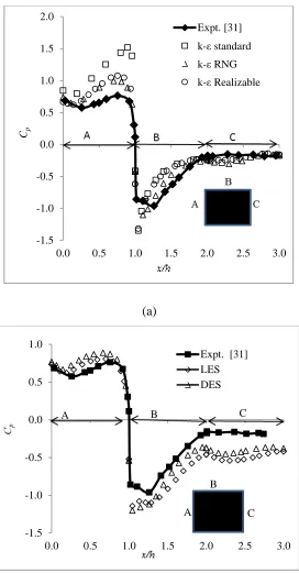
a). Windward symmetry plane

The k-ω-SST model shows the best performance for the prediction of Cp on the front of

the cube, closely matching with experimental data as seen in Fig. 2-6a. The Reynolds

Stress Model ranks second, as illustrated in Fig. 2-6b. Although it could not predict the

Cp increase near the ground level, which is due to the effect of front wall recirculation,

for most of the front face, RSM yields a good overall prediction. The least accurate

prediction is the k-ω standard result which, as shown in Fig. 2-6a, over-predicts Cp by

four-fold. The second worst performance is k-ε standard (Fig. 2-7a), over-predicting Cp

(36)

15

for this will be discussed in section 2.8.2. The Spalart-Allmaras model (Fig. 2-6b), k-ε

RNG and k-ε Realizable (Fig. 2-7a) have similar performance., all of them predict the correct shape of the Cp curve only slightly over-predict the Cp near the leading edge

region. Both DES-SST and LES (Fig. 2-7b) accurately predict Cp on the windward face,

although LES appears slightly closer to the experimental data.

b). Roof symmetry plane

Considering only the roof portion of the cube, RSM has the best prediction of Cp, closely

matching the experimental data (Fig. 2-6b); k-ω-SST and k-ε RNG also both give good prediction on the roof. The k-ɷ-SST model slightly under-predicts the suction pressure near the leading edge, while k-ε RNG slightly over-predicts the suction pressure. The SA model over-predicts the suction pressure near the leading edge and under-predicts it over

the main region. The k-ω standard, k-ε standard and k-ε Realizable fail to predict the Cp

on the roof; they significantly over-predict the suction pressure on the leading edge and

under-predict the suction pressure in the remaining region. Both DES-SST and LES

slightly over-predict the suction pressure on the roof, but still are in an acceptable range.

DES-SST results appear to be closer to the experimental data than LES.

c). Leeward symmetry plane

On the leeward side, the experimental Cp shows constant negative value (around -0.2)

from the top of the cube to ground level in the symmetry plane, while all the RANS

models show only a slight deviation from this constant value. In general, all the RANS

models not only have similar performance but also are very close to the experimental data.

(37)

16

(a)

(b)

Fig. 2-6 Cp distribution at vertical symmetry plane from (a) k-ω standard and k-ω-SST

models; (b) Reynolds Stress Model (RSM) and Spalart-Allmaras (SA) model

-1.5 -1.0 -0.5 0.0 0.5 1.0 1.5 2.0 2.5 3.0

0.0 0.5 1.0 1.5 2.0 2.5 3.0

Expt. [31]

k-ɷ-SST

k-ɷ standard

-1.5 -1.0 -0.5 0.0 0.5 1.0 1.5

0.0 0.5 1.0 1.5 2.0 2.5 3.0

(38)

17

(a)

(b)

Fig. 2-7 Cp distribution at vertical symmetry plane from (a) k-ε standard, k-ε RNG and k-ε

Realizable models; (b) DES–SST and LES (dynamic Smagorinsky) models

-1.5 -1.0 -0.5 0.0 0.5 1.0 1.5 2.0

0.0 0.5 1.0 1.5 2.0 2.5 3.0

Expt. [31]

k-ε standard

k-ε RNG

k-ε Realizable

Cp

-1.5 -1.0 -0.5 0.0 0.5 1.0

0.0 0.5 1.0 1.5 2.0 2.5 3.0

Expt. [31] LES DES

A B

C

(39)

18

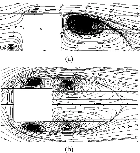
2.8.2 Flow Pattern around the Cube

The streamtraces pattern near the cube in the vertical symmetry plane and a horizontal

plane near the ground, predicted by the seven RANS models, DES-SST and LES, are

presented in Figs. 2-8 to 2-16. Most models have predicted the ring vortex, roof

separation bubble, side separation and wake recirculation, but the shapes and locations

are different from each other. As seen in Fig. 2-9a and Fig. 2-12a, both k-ε standard and

k-ω standard fail to predict the roof separation. This is the reason that the predicted Cp

from these models rises to a value greater than 1. The flow patterns from RANS models

are more symmetrical than those from DES-SST and LES. The reason for this may be

that the simulation times for the DES-SST and LES are not long enough. Since there is

no experimental information about the streamtraces pattern, one should be cautious to

speculate which model predicts the more realistic flow pattern. Nevertheless, based on

the Cp discussions above, it appears that the k-ω-SST provides the most reliable results

over the entire cube.

(a)

(b)

Fig. 2-8 Streamtraces predicted by Spalart-Allmaras model, (a) vertical symmetry plane;

(40)

19

(a)

(b)

Fig. 2-9 Streamtraces predicted by k-ε standard model, (a) vertical symmetry plane; (b) horizontal plane at 0.125h

(a)

(b)

(41)

20

(a)

(b)

Fig. 2-11 Streamtraces predicted by k-ε Realizable model, (a) vertical symmetry plane; (b) horizontal plane at 0.125h

(a)

(b)

(42)

21

(a)

(b)

Fig. 2-13 Streamtraces predicted by k-ω-SST model, (a) vertical symmetry plane; (b) horizontal plane at 0.125h

(a)

(b)

Fig. 2-14 Streamtraces predicted by Reynolds Stress Model, (a) vertical symmetry plane;

(43)

22

(a)

(b)

Fig. 2-15 Streamtraces predicted by DES-SST model, (a) vertical symmetry plane;

(b) horizontal plane at 0.125h

(a)

(b)

Fig. 2-16 Streamtraces predicted by LES (dynamic Smagorinsky), (a) vertical symmetry

(44)

23

2.8.3 Flow Recirculation Length

Unfortunately, there is no reported experimental data about the recirculation length for

the reattachment behind the cube. The flow recirculation length predicted by different

models has been summarized in Table 2.2. From this table, one can see that the

recirculation length predicted from the RANS models is larger than that from DES or

LES. This observation is consistent with information reported in the literature [27], where

the result from LES is closer to experimental data in the case of a square cylinder.

Table 2.2 Flow recirculation length in the wake region (h: cube height)

Model Recirculation length

Spalart-Allmaras 1.80h

k-ω standard 1.75h

k-ω-SST 2.25h

k-ε standard 1.63h

k-ε RNG 1.95h

k-ε Realizable 1.85h

Reynolds Stress 1.80h

DES-SST 1.35h

LES (Dynamic Smagorinsky) 1.50h

2.9 Discussion and Conclusions

As mentioned above, there is less information reported in the literature about numerical

simulations over cubes with unstructured meshes, for both RANS models and LES. The

main reasons may be the ineffective discretization of space with an unstructured mesh

and the general lack of familiarity of unstructured meshes in this type of application.

Nevertheless, through construction of the computational model and setting up of the mesh,

we have found that the unstructured mesh is much more flexible than a structured mesh.

However, successful implementation of an unstructured mesh requires good experience

using some important mesh parameters, such as cell growth rate, maximum cell size and

(45)

24

The simulation results from both DES-SST and LES are not as good as those from k-ω -SST and RSM. This may be due to the fact that the mesh near the cube is still too coarse

for the LES case. Usually the y+ value required for LES is around 1 [22], which consequently requires huge computing power for the high Reynolds number in the

current simulations. Although the Werner-Wengle wall function has been implemented, it

may be that the mesh is still too coarse to capture the near-wall region with the current

mesh methodology. For the DES case, the communication between the RANS model and

the LES model at the interface might be an issue affecting the prediction accuracy.

Computational domain size of type A is too small, and the boundary conditions will

greatly affect the simulation results on both the roof and leeward side of the cube. Type B,

which is recommended by the Best CFD Performance Guide [6], is acceptable for the

simulation results when compared with a larger domain size such as type C, since type C

domain will only slightly improve the results on the roof region, and does not change the

results on either the windward or leeward sides.

Amongst the RANS model mentioned in this chapter, both k-ω-SST and the Reynolds Stress Model are the most suitable models to predict wind load on a building. They

accurately predict the pressure coefficient on the windward wall, the roof and on the

leeward wall. The Reynolds Stress Model needs much more computing power than the k-ω-SST model. The k-ε standard, k-ε Realizable and k-ω standard are not suitable for bluff body flow simulations. Spalart-Allmaras model and k-ε RNG give similar prediction performance, and compare reasonably well with experimental data.

In this thesis, the velocity field obtained from the numerical simulations has not been

compared with experimental data. The velocity field predictions are usually more

accurate than the pressure field. However, for the current purpose, the pressure

distribution is more important than the velocity field in regards to the final objectives of

this thesis. It is also important to keep in mind that both the wind tunnel tests and the

(46)

25

CHAPTER 3 Wind Load on a Free Standing Roof in an

Atmospheric Boundary Layer

The effects of turbulence modeling on the numerical simulation of wind load on a free

standing roof are investigated in this chapter. The main objective is to predict the wind

load on the mid-section of a free standing inclined roof, also referred to as a canopy,

under atmospheric boundary layer flow. Nine turbulence models are considered, seven

Reynolds-Averaged Navier-Stokes (RANS) equation models, Large-eddy Simulation

(LES) with dynamic Smagorinsky subgrid model and Detached Eddy Simulation

(DES-SST). The RANS models are Spalart-Allmaras (SA), k-ε standard, RNG and Realizable,

k-ω standard, k-ω-SST and Reynolds Stress Model (RSM). The difference in mean pressure coefficient (Cp) across the roof, at different wind directions, obtained from each

RANS model with two levels of mesh fineness, has been compared with experimental

data.

3.1 Flow Problem Description

For the current study, wind tunnel test data corresponding to an atmospheric boundary

layer for a suburban terrain has been extracted from literature [8]. A schematic of the

flow problem is shown in Fig. 3-1. The full-scale dimension of the canopy is 30 m x 30 m,

with roof slope of 22.5o and support height of 10 m. The model scale in the numerical

model is the same as in the wind tunnel test, 1:100. Velocity and streamwise turbulence

intensity profiles at the location of the canopy, but without the presence of the canopy,

are shown in Fig. 3-2 and Fig. 3-3, respectively. For consistency with the experiments,

the velocity in Fig. 3-2 is normalized by the velocity at 60 m in real scale, u60.

(47)

26

Fig. 3-1 Geometry of canopy with 0o wind attack angle

Fig. 3-2 Velocity profile near canopy location

Fig. 3-3 Turbulence intensity profile in streamwise direction near canopy location

0.0 0.1 0.2 0.3 0.4 0.5 0.6

0.0 0.2 0.4 0.6 0.8 1.0 1.2

Expt. [8] k-ɷ-SST RSM (m) z x 1 0 -2 0.00 0.10 0.20 0.30 0.40 0.50

0.00 0.20 0.40

Expt. [8]

k-ɷ-SST

(48)

27

3.2 Governing Equations

The equations that govern the unsteady flow of an incompressible fluid are [35]

𝜕𝑢𝑖

𝜕𝑥𝑖 = 0 (3-1)

𝜌𝜕𝑢𝑖

𝜕𝑡 +𝜌 𝜕(𝑢𝑗𝑢𝑖)

𝜕𝑥𝑗 = −

𝜕𝑝 𝜕𝑥𝑖+

𝜕 𝜕𝑥𝑗(𝜇

𝜕𝑢_𝑖

𝜕𝑥𝑗) (3-2)

where ui, p, ρ and µ denote the velocity components in the Cartesian coordinate system

xi , (i = 1, 2, 3), pressure, density and dynamic viscosity, respectively.

These equations are the same as those used in Chapter 2. A discussion of the turbulence

models used with these equations can be found in section 2.2 and a detailed description of

these models is given in Appendix A. Discussion of the wall treatment and

implementation of different models is provided in Appendix B.

3.3 Computational Domain

The horizontal and cross-section layouts of the computational domain are illustrated in

Fig. 3-4 and Fig. 3-5, respectively, where h is the height of the canopy support.

(49)

28

3.4 Boundary Conditions

The boundary conditions associated with the flow over the canopy are identical to those

for flow over the cube building. These conditions are discussed in section 2.5 and

mathematically formulated as equations (2-3) to (2-7).

3.5 Mesh Topology

A tetrahedral mesh, with two levels of refinement, is used for the RANS models. For the

coarse mesh, the smallest cell size is around 15 mm in the region near the canopy, while

in the far region the cell size is around 70 mm, with total cell number of approximately

150,000. For the finer mesh, the smallest cell size is around 7 mm in the region close to

the canopy, with 70 mm cell size farther away, with a total of approximately 300,000

cells. The DES and LES models will only be implemented on the coarse mesh due to the

computational power limitation. The fine mesh (7 mm) in the vicinity of the canopy is

shown in Fig. 3-5.

Fig.3-5 Tetrahedral mesh around the canopy in the cross-section layout

3.6 Numerical Setup

The numerical setup for this problem is the same as that for the cube building in Chapter

2. Except for RSM, the convective terms in the RANS models are discretized with

(50)

29

solution algorithm uses pressure based, pressure-velocity coupling. For RSM, the

second-order upwind scheme is used for convection terms, while the solution algorithm uses

pressure based, segregated and SIMPLE [24]. Bounded central differencing is used for

momentum equations in the LES and DES simulations. The time discretization is implicit

second-order. The drag coefficient and a continuity equation residual less than 10-7 have

been used as the converge criteria.

3.7 Simulation Results

3.7.1 Wind Load on the Canopy Roof

Throughout this chapter, the pressure coefficient refers to the area-averaged pressure

coefficient. The pressure coefficient difference on the middle section of the windward

roof, i.e., on plate e in Fig. 3-1, with wind attack angles from 0o to 180o, has been

predicted using the seven RANS models, as well as the DES-SST model and the LES

dynamic Smagorinsky model. The pressure coefficient difference, ∆Cp, is defined as the

difference between the pressure coefficient on the top surface and on the bottom surface

of the roof, that is

∆𝐶𝑝 =(1𝑝𝑇−𝑝𝐵) 2𝜌𝑢𝑟𝑒𝑓2

(3-3)

where pT and pB are the area-averaged pressures on the top and bottom of the roof,

respectively. Positive ∆Cp means that the roof plate experiences a downward force, while

a negative ∆Cp indicates an upward force.

a). Simulation results from k-ω, k-ω-SST and Spalart-Allmaras (SA) model

The variations of ∆Cp on plate e, extracted from the coarse mesh simulations (15 mm cell

size around the canopy) using the k-ω standard, k-ω-SST and Spalart-Allmaras models, are plotted in Fig. 3-6, demonstrating that the k-ω-SST and Spalart-Allmaras models have much better accuracy than the k-ω standard model in the windward attack direction (from 0o to 90o). The k-ω-SST and SA simulation results at these wind attack angles display good agreement with the experimental data of Ginger and Letchford [8], except for wind

(51)

30

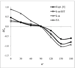
and SA show around 25% deviation from experimental data. The k-ω standard model results are even less reliable, as seen in Fig. 3-6.

Fig. 3-6 ∆Cp at different wind attack angles predicted by RANS models

(coarse mesh near the canopy)

With a finer mesh (7 mm cells around the canopy), k-ω-SST and SA models show no improvement at windward attack angles. Figure 3-7 illustrates that, although the k-ω

standard model shows noticeable improvement, particularly at 0o, it still deviates much

more from experimental data compared to the other two models. On the leeward side, all

three models show obvious improvement only at 180o attack angle. Among these three

models, the k-ω-SST shows slightly better prediction than the SA model, and much better than the k-ω standard model. It yields good prediction at wind attack angles from 30o up to 90o, then starts to deviate from the experimental data from 90o and reaches maximum

deviation at 150o wind attack angle, after which the difference decreases. At 180o, the k-ω-SST model gives good prediction of ∆Cp. In both levels of mesh refinement, all the

models show the correct ∆Cp prediction at 90o wind attack angle. As seen in Fig. 3-7, -1.5

-1.0 -0.5 0.0 0.5 1.0

0 30 60 90 120 150 180

Expt. [8]

k-ɷ-SST

k-ɷ

SA

Δ

Cp

(52)

31

none of these three models show improvement with mesh refinement at wind attack

angles around 150o.

Fig. 3-7 ∆Cp at different wind attack angles by RANS models

(fine mesh near the canopy)

b). Simulation results from k-ε standard, k-ε RNG, k-ε Realizable and Reynolds Stress Model (RSM)

Figure 3-8 illustrates the coarse mesh results for this family of k-ε models and RSM. The behaviour of RSM is quite different from the k-ε models. At windward attack angles between 0o and 60o, both RSM and k-ε standard show significant deviation in the ∆Cp

values from the experimental data, while k-ε RNG gives relatively better prediction and Realizable gives reasonably good results. In the leeward wind attack angles from 90o to

180o, the RSM model gives much better prediction than the other three models, but the

difference between the RSM results and experimental data is still noticeable, especially

for wind attack angles between 120o to 180o. The k-ε standard model gives the least accurate prediction among the four models.

-1.5 -1.0 -0.5 0.0 0.5 1.0

0 30 60 90 120 150 180

Expt. [8]

k-ɷ-SST

k-ɷ

SA

Δ

Cp

(53)

32

Fig. 3-8 ∆Cp at different wind attack angles by RSM, k-ε standard, RNG, Realizable

(coarse mesh near the canopy)

Using the finer mesh, there is no improvement in the simulation results of RSM for wind

direction from 0o to 60o. As seen in Fig. 3-9, k-ε RNG and k-ε Realizable improve at 30o and 60o, but still deviate at 0o. None of these models can accurately capture the ∆Cp

variation with the change of wind attack angle. The simulation result of k-ε standard has improved with the refined mesh. In leeward wind attack angles, the RSM results show

improvement only at 180o. The simulation results from k-ε RNG and k-ε Realizable do not improve at any leeward wind attack angle. Figure 3-9 shows that the k-ε standard simulation has improved slightly at wind attack angle of 180o.

-1.5 -1.0 -0.5 0.0 0.5 1.0

0 30 60 90 120 150 180

Expt. [8] RSM

k-ε standard

RNG Realizable

Δ

Cp