The Economic Lot Scheduling Problem: Exact Solutions and System Feasibility.

ABSTRACT

HANSON, BRIAN BENNETT. The Economic Lot Scheduling Problem: Exact Solutions and System Feasibility. (Under the direction of Dr. Thom J. Hodgson and Dr. Russell E. King).

The Economic Lot Scheduling Problem considers the single-machine, multi-product

inventory system. The objective is to determine a production schedule which minimizes

long-run inventory and setup costs while avoiding stock outs. The problem is NP-hard (Hsu,

1983). This has led to a variety of simplifying assumptions and scheduling heuristics. First,

this thesis demonstrates that exact solutions can be obtained under the basic period

assumption using the benchmark Bomberger problem. Second, a generalization of the

“power-of-two” method, called the “power-of-primes,” is introduced. An algorithm,

motivated by the methodology of part I, is developed which obtains exact solutions under

both the power-of-two and power-of-prime assumptions. Solutions are shown to be superior

to existing methods for a variety of real-world parameters. Third, an analytical method is

presented which determines the set of all inventory positions from which it is possible to

avoid a stock out over the infinite time horizon (the “feasible region”). Similar methods are

© Copyright 2013 Brian B. Hanson

The Economic Lot Scheduling Problem: Exact Solutions and System Feasibility

by Brian B. Hanson

A dissertation submitted to the Graduate Faculty of North Carolina State University

in partial fulfillment of the requirements for the degree of

Doctor of Philosophy

Operations Research

Raleigh, North Carolina

2014

BIOGRAPHY

Brian Bennett Hanson is a native of Traverse City, Michigan. He received a B.S. in

Mathematics from Grand Valley State University (2006) and a M.S. in Mathematics from

Miami University (2008). Brian enrolled in the Operations Research Ph.D. program at North

ACKNOWLEDGMENTS

I would like to acknowledge the guidance of the mathematics faculty of Northwestern

Michigan Community College, Grand Valley State University, and Miami University who’s

dedication to teaching is responsible for my continued studies. Specifically, Dr. Stephen

Drake, NMC, who inspired me to pursue mathematics, Dr. Paul Fishback, GVSU, who

encouraged me to continue my studies in graduate school, and my Master’s advisor Dr. Zevi

Miller, MU, who first guided me through the research process. I would also like to

acknowledge Dr. Thom Hodgson for spending the last three years challenging my

mathematical training until, I hope, I reached the point where I can “think like a

mathematician” or “think like an engineer” with equal ability. Finally, I would like to

acknowledge the rest of my thesis committee, Dr. Michael Kay, Dr. Russell King, and Dr.

TABLE OF CONTENTS

LIST OF TABLES ... vi

LIST OF FIGURES ... vii

Chapter 1 Introduction ...1

Chapter 2 On the Lot Size Scheduling Problem, Part I: The Optimal Solution to the Bomberger data ...3

1 Introduction ...3

2 Literature Review ...4

3 Exact Solution for Bomberger’s Data ...5

3.1 Bounds on Cost and Cycle Time ...5

3.2 Bounds on the Basic Period ...7

3.3 Bounds on the Multipliers ...7

3.4 Partitioning the Basic Period into Intervals ...7

3.5 A Search Method for Basic Period Intervals ...8

3.5.1 Schedule Feasibility Conditions ...9

3.5.2 Partial Example...11

3.6 Analysis of the Remaining Basic Period Intervals ...11

4 Conclusion ...13

CHAPTER 2 REFERENCES ...14

CHAPTER 2 APPENDIX ...16

Chapter 3 On the Lot Size Scheduling Problem, Part II: Determining Exact Solutions to the ELSP under the Power-of-Two and Power-of-Prime Assumptions ...19

1 Introduction ...19

2 Literature Review ...21

3 Practical Motivation ...22

4 Methodology ...23

4.1 Upper and Lower Bounds on the Basic Period (𝑻) ...24

4.2 Determining all 𝒌 with a (potentially) lower cost given 𝒃 ≤ 𝑻 ≤ 𝒃+𝜹 ...26

4.3 Determining the existence of a feasible production schedule given (𝒌,𝑻) ...26

4.4 Mathematical Preliminaries ...27

4.5 Determining 𝝉𝝅 (the maximum time required to setup and produce all products 𝒋 where 𝒌𝒋 is a power of 𝝅 in any basic period ...34

5 Experimentation ...42

5.1 Bomberger Data ...42

5.2 Experimental Design ...43

5.3 Note on choice of the Experimental Design ...44

5.4 Results ...46

6 Conclusion ...48

CHAPTER 3 REFERENCES ...50

Chapter 4 On the Lot Size Scheduling Problem, Part III: Stock Out Prevention and

System Feasibility...59

1 Introduction ...59

2 Literature Review ...60

3 Delaying a Stock Out ...63

3.1 Preliminaries ...64

3.2 Feasibility Condition on the Total Production Plus Setup Time ...65

3.3 Procedure to Determine 𝒕 Given 𝑻,𝒇, and 𝑰 ...66

3.4 Analytical Alternative to Solve the SAP...69

3.5 Algorithm to Determine Maximum 𝑻 given 𝒇 and 𝑰 ...70

3.6 Search Procedure to Determine Maximum 𝑻 given 𝑰 ...71

3.7 Heuristic to Determine Maximum 𝑻 given 𝑰 ...71

4 Inventory Recovery ...74

4.1 Method to Determine 𝒕 given 𝑻,𝒇,𝑰, and 𝑼 ...74

4.2 Search to Determine 𝒇 and 𝒕 given 𝑻,𝑰, and 𝑼 ...75

4.3 Determining the Minimum 𝑻 Given 𝑰 and 𝑼 ...75

5 The Feasible Region ...76

6 Conclusion ...82

CHAPTER 4 REFERENCES ...83

CHAPTER 4 APPENDICES ...86

Chapter 5 Conclusion ...89

LIST OF TABLES Chapter 2

Table 1: Lower and Upper Bounds on Cycle Time...6

Table 2: Feasible Partial Schedules ...12

Table 3: Bomberger’s Data ...17

Table 4: Re-Ordering of Products ...17

Table 5: Possible values k for 23.6≤ 𝑇 ≤23.7 ...17

Table 6: Interaction of “2 groups” and “3 groups” ...18

Chapter 3 Table 1: Total Time by Period ...29

Table 2: Partitions of 5 products into set of 3 and set of 2 ...35

Table 3: Partitions of 6 products into set of 4 and set of 2 ...36

Table 4: Partitions of 6 products into two sets of 3 ...37

Table 5: Partitions of 8 products into set of 3 and two sets of 2 ...38

Table 6: Comparison P2, PP, GA for Bomberger’s Data ...43

Table 7: Experimental Design ...44

Table 8: Five Product Results ...47

Table 9: Ten Product Results ...47

Table 10: P2 and PP Optimal k’s for Bomberger’s Problem ...48

Table 11: Partitions of 7 products into set of 5 and set of 2 ...53

Table 12: Partitions of 7 products into set of 4 and set of 3 ...53

Table 13: Partitions of 8 products into set of 4 and two sets of 2 ...54

Table 14: Partitions of 8 products into two sets of 3 and set of 2 ...54

Table 15: Partitions of 8 products into set of 6 and set of 2 ...55

Table 16: Partitions of 8 products into set of 5 and set of 3 ...55

Table 17: Partition of 9 products into set of 5 and two sets of 2 ...56

Table 18: Partition of 9 products into set of 4, set of 3, and set of 2...56

Table 19: Partition of 8 products into three sets of 3 ...57

Table 20: 𝜂₉ = 8 using six basic periods ...57

Chapter 4 Table 1: Data for Anderson’s (1990) Example ...69

Table 2: Computational Times for Heuristic (seconds) ...74

Table 3: Percent of the Feasible Region ...81

LIST OF FIGURES Chapter 2

Figure 1: Total Cost vs. Cycle Time of Product 1 ...6

Chapter 3 Figure 1: Total Cost vs. Cycle Time of Product 1 of the Bomberger Data ...25

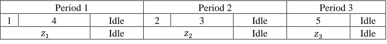
Figure 2: Illustration of 𝑧1,𝑧2,𝑧3 for [14|23|5] ...40

Figure 3: Adding products with 𝑘_𝑗 = 9 to an existing 3-period schedule...40

Figure 4: Total Cost vs. Utilization ...46

Chapter 4 Figure 1: Section 3 (Diagrammatically) ...64

Chapter 1

Introduction

The Economic Lot Scheduling Problem (ELSP) considers a single-machine, multi-product

inventory system. The machine is assumed to be capable of producing one product at a time,

and requires a setup time before producing each product. A “production schedule” is

required which indicates the order (production sequence) and quantity (lot size) in which to

produce the products. The objective is to determine a cyclic (repeatable) production schedule

which minimizes long-run inventory and setup costs.

In practice, variations in demand, machine disruptions, and other inconveniences of

every day plant life prevent the cyclic production schedule from being implemented exactly

as designed. As observed by Bomberger (1966), “repetitive schedules that call for the same

quantity of an item to be made in each cycle cannot be strictly maintained in reality,” but “it

is often possible to adjust production to correct for such disturbances.” Instead, the cyclic

schedule is used as a “first attempt at a feasible schedule which can then be manipulated to

meet the detailed requirements of the shop floor” (Anderson, 1990). Essentially, the

production schedule acts as a “production plan” rather than a strict schedule.

Occasionally, a machine disruption or another event may be significant enough that

the cyclic production schedule cannot easily be modified to meet demand. If inventory levels

become critically low, the system is in danger of a stock out occurring. In practice, a stock

out may prevent the rest of the production facility from operating (i.e. “put the line down”),

and is considered an extremely adverse event (Hodgson, 1980). Therefore, if inventory

levels are low, the principle concern of the manager is avoiding a stock out (not minimizing

cost.

The ELSP was first formally posed by Rogers (1958) and has been the object of

extensive study. The problem is NP-hard (Hsu, 1983), and various simplifying assumptions

have been made to find economic cyclic schedules. The primary focus in the literature has

been the development of various heuristics to find economic cyclic schedules. This thesis

production sequences and obtain the exact optimal solution under the basic period

assumptions. Insights gained from this example lead to a generalization of the power-of-two

method called the “power-of-primes.” An algorithm, motivated by the methodology of part

I, is developed which obtains exact solutions to the general ELSP under the power-of-primes

assumptions (and, consequently, the exact solutions under the power-of-two assumptions).

Solutions are shown to be superior to existing methods for a variety of real-world parameters.

Finally, the situation where inventory levels are critically low is addressed using three

analytical methods. One method determines the set of all inventory positions from which it

is possible to avoid a stock out over the infinite time horizon. This set is called the “feasible

region.” The remaining two methods address the cases where the initial inventory is in the

feasible region, and the case where the initial inventory is not in the feasible region. For the

first case, the minimum time required to obtain sufficient inventory to apply a desired cyclic

schedule is found. In the second, the maximum time that a stock out can be avoided is

determined.

The body of this paper consists of three papers. The first paper proves the solution to

the Bomberger problem found by Doll and Whybark (1973) and Haessler and Hogue (1976)

is optimal. The second paper develops the power-of-primes method. The third paper

contains the three analytical methods to address the situation inventory levels are critically

Chapter 2

On the Lot Size Scheduling Problem, Part I: The Optimal

Solution to the Bomberger

data

Abstract: The Economic Lot Scheduling Problem (ELSP) is a classical scheduling problem with the objective of minimizing the long-run inventory and setup costs of a single machine, multi-product inventory system. A classical data set of ten “more or less typical metal stampings” was presented by Bomberger in 1966. The data set has been extensively studied by numerous authors including Doll and Whybark in 1973, and Haessler and Hogue in 1976. This note determines the exact solution to

Bomberger’s data under the basic period assumptions, proving that the solution found by Doll and Whybark, and Haessler and Hogue is optimal.

1 Introduction:

The Economic Lot Scheduling Problem (ELSP) consists of a single machine assigned to

produce 𝑛 products. The machine is only capable of producing a single product at a time and requires a “setup” before a product can be produced. The daily demand rate of product 𝑗 is

𝑑𝑗, the daily production rate is 𝑝𝑗, and the setup time in days is 𝑠𝑗 for 𝑗 = 1, …𝑛. Each time

the machine is setup for product 𝑗, a cost of 𝑎𝑗 is incurred. The unit cost of product 𝑗, 𝑐𝑗, is the combined material and production cost. Additionally, there is a daily internal inventory

cost rate of $i /$ inventory/day that is proportional to the on-hand inventory. All parameters

are assumed to be known constants and are independent of the order in which the products

are produced. The task is to find a lot size-schedule which minimizes long run inventory and

setup costs while satisfying demand (stock outs are not allowed).

The ELSP is NP-hard (Hsu, 1983) and no known method to obtain the exact solution

exists. Bomberger (1966) introduced the “basic period” approach which considers a

restricted version of the problem (also NP-hard, Hsu, (1983)). The restricted problem

assumes that each production run of product 𝑗 has the same lot size (equal lot sizes), and that each time product 𝑗 begins production, the inventory of product 𝑗 is zero (zero-switch rule). The combination of equal lot sizes and the zero-switch rule imply that the production runs of

period” approach assumes that there is a fundamental cycle time referred to as the basic

period (𝑇). Each product is assumed to be produced every 𝑘_𝑗𝑇 time units, where 𝑘𝑗 is a dimensionless integer. The basic period 𝑇 and the 𝑘_𝑗’s (sometimes referred to simply as “multipliers”) are variables and determine the lot size of each product.

A classical data set of ten “more or less typical metal stampings” was presented by

Bomberger (1966). This data set has been extensively studied by numerous authors

including Doll and Whybark (1973) and Haessler and Hogue (1976). The primary

contribution of this note is to prove that the schedule provided by both Doll and Whybark

(1973), and Haessler and Hogue (1976) is in fact the optimal solution for Bomberger’s data.

2 Literature Review:

A great deal of literature exists on the ELSP. Bomberger’s data has been used by a number

of authors as a benchmark for the performance of their heuristics. This literature review is

limited primarily to papers published on the ELSP prior to 1966 and those which use the

Bomberger (1966) data.

The ELSP was formally posed by Rogers (1958). Rogers introduced the Independent

Solution approach which determines optimal lot sizes for each product without regard to the

fact that all the products must be produced on the same machine. Conflicts naturally arise

when more than one product is scheduled to be produced at the same time. A heuristic is

used to adjust lot sizes and startup times to resolve the conflicts.

The Common Cycle or Rotation Cycle approach was first introduced by Hanssmann

(1962) and Elion (1962). Each product is assumed to be produced once during a fixed time

effective for low to medium loads. Stankard and Gupta (1969) propose a “grouping”

procedure. The products for which it would be economically advantageous to produce more

frequently form group “A” and the other products are divided into groups “B”, “C”, and “D”.

The groups, rather than the individual products, are then scheduled. Hodgson (1970) uses a

pseudo dynamic programming procedure to improve the optimization. Doll and Whybark

(1973) developed an iterative procedure to determine the multipliers for the BP approach.

Schweitzer and Silver (1983) demonstrate the need for a lower bound on the basic period to

insure Doll and Whybark’s solution is feasible. For additional references on the limitations

and feasibility of BP solutions see Haessler and Hogue (1976) and Andres and Emmons

(1976). Haessler and Hogue (1976) also introduce a “power-of-two” method which restricts

the multipliers to a power of 2 (i.e. 𝑘_𝑗 = 2𝑚 for some 𝑚). A survey and the extended BP approach are provided by Elmaghraby (1978).

3 Exact Solution for Bomberger’s Data:

The Bomberger (1966) data can be found in Table 3 in the Appendix. Without loss of

generality, the products are re-numbered for the convenience of the reader in order to

facilitate a depth first search (See Table 4 in the Appendix), which will become relevant later

in the paper. In this section, bounds on cost, cycle time, the basic period, and on multipliers

are presented. Next, the basic period is partitioned into intervals, and bounds on the

multipliers are recomputed. For each interval, the remaining multipliers are searched. This

eliminates multipliers whose lower bound on cost is greater than the cost of the best known

solution, or do not satisfy the feasibility conditions (see Section 3.5.1). The remaining

multipliers are then analyzed to find the optimal solution.

3.1 Bounds on Cost and Cycle Time:

The total cost rate of the best known solution is $32.07/day. A well-known lower bound on

the total cost is the sum of the costs assuming that each product is run using the Economic

Lot Quantity (ELQ), Rogers (1958). The lower bound on the total cost for the Bomberger

data is

In order to determine the optimal solution, all schedules with a total cost less than $32.07/day

need to be considered. There is a total of 32.07-31.62 =$0.45/day “slack” between the lower

bound and the best known solution. In order for the total cost to be less than $32.07, each product can cost no more than

0.45 +�2𝑑𝑗𝑎𝑗𝑖𝑐𝑗(1− 𝑑𝑗/𝑝𝑗), for 𝑗 = 1, … ,10. (2) Since the total cost of product 𝑗 is a convex function of product 𝑗’s cycle time, 𝑡_𝑗, the range of cycle times in which the total cost is less than the amount computed in Equation 2

can be easily found. Thus, the upper bound on the cost of an individual product j can be used

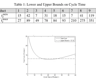
to obtain an upper bound, 𝑡_𝑗𝑚𝑎𝑥, and lower bound, 𝑡_𝑗𝑚𝑖𝑛, on the cycle time of each product 𝑗. For example, by applying Equation 2, product 1 can cost at most $13.12/day. This implies

that the cycle time of product 1 must be between 15 and 27 (see Figure 1 below). The upper

and lower bounds on the cycle times computed in this manner can be found in Table 1. Note

that 𝑡_𝑗𝑚𝑖𝑛 is rounded down and 𝑡_𝑗𝑚𝑎𝑥 is rounded up in the table to include the entire interval.

Table 1: Lower and Upper Bounds on Cycle Time

Product 1 2 3 4 5 6 7 8 9 10

𝑡𝑗𝑚𝑖𝑛 15 42 7 31 18 15 7 41 119 24

3.2 Bounds on the Basic Period:

In this section, an upper bound, 𝑇𝑚𝑎𝑥, and a lower bound, 𝑇𝑚𝑖𝑛, on the basic period are found. Because the cycle time of product 𝑗 is 𝑡_𝑗 = 𝑘_𝑗𝑇, each product’s cycle time is greater than or equal to the basic period (𝑡_𝑗 ≥ 𝑇 ∀𝑗). Therefore, the upper bounds on the 𝑡_𝑗’s are upper bounds on T (𝑡_𝑗𝑚𝑎𝑥 ≥ 𝑡_𝑗 ≥ 𝑇 ∀𝑗). Thus an upper bound on T is

𝑇𝑚𝑎𝑥 _{= min} 𝑗 �𝑡𝑗

𝑚𝑎𝑥_{�. (3)}

For Bomberger’s data, 𝑇𝑚𝑎𝑥 = 27.

The lower bounds on the cycle times can be used to obtain a lower bound on the basic

period since the basic period has to be long enough to setup and produce a product for its

minimum cycle time. Thus, a lower bound on T is

𝑇𝑚𝑖𝑛 _{= max} 𝑗 �𝑠𝑗+

𝑡𝑗𝑚𝑖𝑛 𝑑𝑗 𝑝𝑗 �

(4)

For Bomberger’s data, the largest minimum setup plus production time is 7.89 for product 2.

Therefore, if the total cost rate is less than or equal to $32.07/day, then 7.89≤ 𝑇 ≤27.

3.3 Bounds on the Multipliers:

Since the cycle time of product 𝑗 is 𝑡_𝑗 = 𝑘_𝑗𝑇, bounds for 𝑡_𝑗 were found in Section 3.1, and bounds for 𝑇 were found in Section 3.2, bounds for multiplier 𝑘_𝑗 can be easily computed. Let 𝑘_𝑗𝑚𝑖𝑛 and 𝑘_𝑗𝑚𝑎𝑥 denote lower and upper bounds on the multipliers of product 𝑗,

respectively. Then

𝑘_𝑗𝑚𝑖𝑛 _=�𝑡𝑗𝑚𝑖𝑛

𝑇𝑚𝑎𝑥� and 𝑘𝑗𝑚𝑎𝑥 = �

𝑡_𝑗𝑚𝑎𝑥 𝑇𝑚𝑖𝑛�

(5a,5b)

However, this results in roughly 7.94 × 1011 possible combinations of multipliers, each of which may result in many more possible schedules.

3.4 Partitioning the Basic Period into Intervals:

In order to make the problem computationally feasible, the interval [7.89,27] is partitioned into subintervals of width 0.1 (with the exception of the first interval which is [7.89,8]). Given that the basic period is contained in the interval [𝑏,𝑏+ 0.1], it may be possible to improve the lower bound on the total cost rate. For example, if the basic period is contained

(which is not possible if the basic period is between 8 and 8.1). Because the cost function is convex, the optimal cycle time of product 3 for the corresponding ELQ problem, given the

basic period is between 8 and 8.1, is either 16.2 or 24 (whichever has the lower cost). In this case, the optimal cycle time is 16.2 and has a total cost rate of 1.0421. This increases the lower bound on the total cost rate for product 3 for the ELSP from 1.0244 to 1.0421. By

applying this process to each product, a new lower bound for the total cost rate for the ELSP

is found. For the interval [8,8.1], the new lower bound is 31.8027 compared to 31.6208. The improved lower bound on cost is used to update the bounds on the cycle time of each

product as in Section 3.1. The updated bounds on the cycle times can be used to update the

𝑘_𝑗𝑚𝑖𝑛_{’s and 𝑘}

𝑗𝑚𝑎𝑥’s as in Section 3.3, with 𝑇𝑚𝑖𝑛 =𝑏 and 𝑇𝑚𝑎𝑥 = 𝑏+ 0.1. This reduces the

possible combinations of multipliers more significantly for some intervals than others. For

example, the number of possible multipliers for the interval [8,8.1] is approximately 5 × 109 where as the number of possible multipliers for the interval [24,24.1] is 3,600.

3.5 A Search Method for Basic Period Intervals:

While the sub-problems are orders of magnitude smaller than the original problem, some

subintervals are still too large to easily be searched to exhaustion. A search procedure is now

developed to address these intervals. At this point, the order of the products becomes

relevant to the efficiency of the procedure. The re-ordering described at the beginning of

Section 3 results in the products being arranged in increasing order from the fewest possible

multipliers to the most (with ties broken arbitrarily). A depth-first search is performed over

the range of feasible multipliers for all intervals. To proceed, the multipliers for the products

multiplier has not yet been selected, and the branch continues to be searched. The procedure

discussed in Sections 3.1 and 3.3 is used to update the bounds on the multipliers.

3.5.1 Schedule Feasibility Conditions:

In this section, the feasibility of a schedule over the interval [𝑏,𝑏+ 0.1] is first discussed. Then, expressions representing the actual and minimum amount of setup plus processing

time incurred in every cycle of length (𝑏+ 0.1) are defined individually for all products with multipliers 1 and 2, respectively. Next, expressions are presented representing the minimum

amount of setup plus processing time incurred in at least one of the 𝑚 groups of length

(𝑏+ 0.1) in which all products with multipliers of 𝑚 are scheduled. Finally, these expressions are combined into necessary feasibility conditions for multipliers from 1 to 6.

In order for the vector of multipliers, k, to lead to a solution, there must exist a feasible schedule (i.e., a schedule where the time required to setup and produce all products

scheduled during each basic period is at most 𝑇). If a schedule is infeasible with basic period

𝑉, then the schedule is infeasible for all 𝑉₀ where 𝑉₀ <𝑉. Thus, if a schedule is infeasible for (𝑏+ 0.1), it is infeasible for any 𝑉 ∈[𝑏,𝑏+ 0.1]. Let

𝜏𝑗 =𝑠𝑗+𝑘𝑗(𝑏+ 0.1)𝑑𝑗_𝑝𝑗 (6)

be the sum of the setup time and the production time to satisfy demand during 𝑘𝑗(𝑏+

0.1) for product j.

Let 𝑓_𝑚be a lower bound on the total time required to setup and produce all products

𝑗 with multiplier 𝑘_𝑗 = 𝑚 in every cycle of length (𝑏+ 0.1) . Since all products with 𝑚=

1 are produced in every cycle, the amount of setup and processing time required for all products with 𝑚= 1 in every cycle of length (𝑏+ 0.1) is

𝑓1 = � 𝜏𝑗 all𝑗,𝑘𝑗=1

. (7)

Any schedule will divide the products with 𝑚 = 2 into two groups. The combined setup and processing time in either group is at most (𝑏+ 0.1). Therefore, a lower bound on the total time required to setup and produce all products with 𝑘_𝑗 = 2 in every cycle of length

𝑓2 = max�0, � (𝜏𝑗) all𝑗,𝑘𝑗=2

−(𝑏+ 0.1) � (8)

Let 𝑔_𝑚 be a lower bound on the total time required to setup and produce all products

𝑗 with multiplier 𝑘𝑗 =𝑚 ≥2 in at least one of the 𝑚 groups in which they are scheduled. Clearly, the product with a multiplier of 𝑚 with the largest total setup and production time

will be in one of the groups. In addition, one of the groups must have at least 1

𝑚of the total

time. Therefore, let

𝑔𝑚 = max�_allmax_𝑗,𝑘

𝑗=𝑚𝜏𝑗,

1

𝑚 � 𝜏_all𝑗,𝑘 𝑗

𝑗=𝑚

�, 𝑚 ≥2. (9)

Combining the expressions defined in Equations 7 thru 9 yields the feasibility

conditions in Equations 10a – d that are used in the search. Because 2 and 3 are relatively

prime, each “2 group” will eventually be scheduled during the same cycle as each “3 group”

(See “Note”, Appendix) (10a). If the multipliers are not relatively prime, then this may not

be the case. For example, a “2 group” may never be scheduled in the same basic period as a

“4 group”. However, 3 and 4 are relatively prime, so each “3 group” will eventually be

scheduled during the same cycle as each “4 group” (10b). Each “2 group”, “3 group”, and “5

group” will eventually be scheduled during the same cycle (10c). In addition, each “3

group”, “5 group”, and “6 group” will eventually be scheduled during the same cycle, but not

necessarily with a 2 “group” (10d).

benefit of potentially terminating a branch. The scarcity of multipliers greater than six in the

Bomberger data made using multipliers less than or equal to six a logical choice.

3.5.2 Partial Example:

The interval [23.6, 23.7] is used as an illustrative example. Initialize 𝑓_𝑚 = 𝑔𝑚 = 0 ∀ 𝑚. The only possible value for 𝑘₁ is 1. The minimum cost for product 1 given that 𝑘₁ = 1 and

23.6≤ 𝑇 ≤23.7 occurs at 23.6. The new lower bound on the cost under these assumptions is the sum of the total cost rate of product 1 with a cycle time of 23.6 and the existing lower

bounds on the total cost rate of the other 9 products. In this case, this does not improve the

lower bound on the total cost rate as 𝑘1 = 1 obtains the previous lower bound for product 1. The value 𝑓₁ is updated to 6.698. Since the lower bound on the total cost, 31.89, is less than the value of the best known solution, 32.07, and none of the constraints (10a-d) are violated,

product 2 is now considered. The possible values for 𝑘₂ are 2 and 3. Arbitrarily choose

𝑘2 = 2 (The case where 𝑘2 = 3 will be considered later in the search.). The updated lower bound on the total cost rate is 32.05. The value 𝑓₂ is updated to 0, and 𝑔₂ is updated to 8.808. Since the lower bound on the total cost is less than the value of the best known solution and

none of the constraints (10a-d) are violated, the search continues. This process can be

repeated until a multiplier has been selected for each product or the branch is fathomed.

Using a depth-first search over all possible multipliers obtains all values of k with a cost less than $32.07/day and 𝑇 ∈ [23.6,23.7] (see Table 5 in the Appendix). This process reduces the 18,000 possible k’s for the interval [23.6, 23.7] to only 23 in less than 0.02 seconds on a 3 GHz machine.

The entire search overall intervals required 0.12 seconds on a 3 GHz machine coded in Matlab. Intervals containing at least one value of k range from 10.9−12.4, 22.5−23.3,

23.4−23.7, and 23.9−24.0.

3.6 Analysis of the Remaining Basic Period Intervals:

The intervals from 10.9−12.4 can be eliminated using the following argument. In each case, 𝑘1 = 2,𝑘2 = 4, and 𝑘3 = 2. There is not sufficient time to setup and produce product 2 and either product 1 or product 3 in the same period. This forces products 1 and 3 to be

products 1 and 3 in the same period. Therefore, none of the intervals between 10.9−12.4 yield values for k which have a feasible schedule and a lower cost than $32.07/day.

Next, the remaining intervals (22.5−23.3,23.4−23.7, and 23.9−24.0) are considered. In each case, 𝑘₁ = 𝑘₃ = 1 and 𝑘₂ =𝑘₄ =𝑘₅ =𝑘₆ =𝑘₇ = 2. Therefore, products 1 and 3 will be setup and produced in every period, and products 2 and 4 − 7 can either be setup and produced in periods 1,3,5,… or 2,4,6,…(i.e. the “odd” or “even” periods)

. Without loss of generality, assume product 2 is setup and produced in the odd periods.

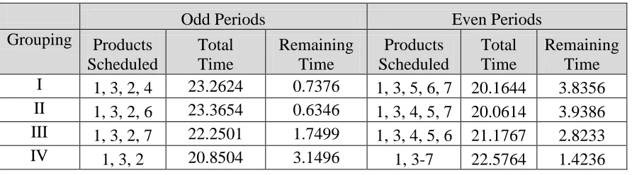
There are 16 distinct ways to schedule products 4 − 7 . For illustrative purposes, the interval

[23.9,24.0] is considered. Table 2 shows the 4 of the 16 ways that are feasible. Each of the three remaining products (8, 9, 10) need to be added to the schedule.

Table 2: Feasible Partial Schedules

Odd Periods Even Periods

Grouping _Products Scheduled

Total Time

Remaining Time

Products Scheduled

Total Time

Remaining Time

I _{1, 3, 2, 4} 23.2624 0.7376 1, 3, 5, 6, 7 20.1644 3.8356

II _{1, 3, 2, 6} 23.3654 0.6346 1, 3, 4, 5, 7 20.0614 3.9386

III _{1, 3, 2, 7} 22.2501 1.7499 1, 3, 4, 5, 6 21.1767 2.8233

IV _{1, 3, 2} 20.8504 3.1496 1, 3-7 22.5764 1.4236

Groupings I, II, and IV have only one period which has sufficient remaining time to

schedule any of the remaining products. If a multiplier is odd, then the product will be

alternate between being produced in the odds periods and even periods. Therefore, 𝑘8,𝑘9, or

𝑘10 cannot be odd. This leaves 𝐤= [1 2 1 2 2 2 2 4 8 6] and 𝐤= [1 2 1 2 2 2 2 4 8 8]. The

first possibility for 𝐤 requires that products 8 and 10 be produced in the same period. However, there is not sufficient time remaining in Groupings I, II, or IV to do this. The

second possibility is the set of multipliers found by Doll and Whybark (1973) and Haessler

and Hogue (1976).

The values vary slightly, but the logic is analogous for the remaining basic period

intervals. In each case, all multipliers except 𝐤∗= [1 2 1 2 2 2 2 4 8 8] are eliminated. The value of 𝑇 (23.42) found by Doll and Whybark, and Haessler and Hogue minimizes cost for

𝐤∗_{. Therefore, the solution found by Doll and Whybark, and Haessler and Hogue is optimal.} 4 Conclusion:

The solution to Bomberger’s data found independently by Doll and Whybark (1973) and

Haessler and Hogue (1976) has been shown to be optimal. The primary approach was to

perform a depth-first search with bounds on the cost being updated and feasibility conditions

CHAPTER 2 REFERENCES

Andres, F.M. and Emmons, H. (1976) On the optimal packaging frequency of products

jointly replenished. Management Science, 22(10), 1165-1166.

Bomberger, E. (1966) A dynamic programming approach to a lot size scheduling problem.

Management Science, 12(11), 778-784.

Doll, C. and Whybark, D. (1973) An iterative procedure for the single-machine multi-product

lot scheduling problem. Management Science, 20(1), 50-55.

Eilon, S. (1962) Elements of Production Planning and Control, Macmillan, New York,

Chapter 10, 227-263.

Elmaghraby, S. (1978) The economic lot scheduling problem (ELSP): review and extensions.

Management Science, 20(1), 50-55.

Haessler, R. and Hogue, S. (1976) A note on the single-machine multi-product lot scheduling

problem. Management Science, 22(8), pp. 909-912.

Hanssmann, F. (1962) Operations Research in Production and Inventory Control, Wiley,

New York.

Hodgson, T.J. (1970) Addendum to Stankard and Gupta’s Note on Lot Size Scheduling.

Schweitzer, P. and Silver, E. (1983) Mathematical pitfalls in the one machine multiproduct

economic lot scheduling problem. Operations Research, 31(2), 401-405

Stankard, M. and Gupta, S. (1969) A note on Bomberger’s approach to lot size scheduling:

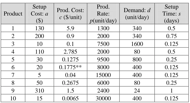
Table 3: Bomberger’s Data*

Product

Setup Cost: a

($)

Prod. Cost:

c ($/unit)

Prod. Rate:

p(unit/day)

Demand: d

(unit/day)

Setup Time: s

(days)

1 130 5.9 1300 340 0.5

2 200 0.9 2000 340 0.75

3 10 0.1 7500 1600 0.125

4 110 2.785 2000 80 0.5

5 30 0.1275 9500 800 0.25

6 20 0.1775** 8000 400 0.125

7 5 0.04 15000 400 0.125

8 50 0.2675 6000 80 0.25

9 310 1.5 2400 24 1

10 15 0.0065 30000 400 0.125

*A single 8-hour shift is run 240 days per year and the inventory carrying cost is

𝑖= $ 0.1/240 /$ inventory/day.

**A data entry error in the Doll and Whybark (1973) paper altered the production cost

rate of product 6 from 0.1175 ($/unit) to 0.1775 ($/unit). This does not affect the optimal

schedule.

Table 4: Re-Ordering of Products

New Product Order 8 9 4 5 3 2 10 6 7 1

Table 5: Possible values 𝐤 for 23.6≤ 𝑇 ≤23.7 (𝑘1 =𝑘3 = 1,𝑘2 = 𝑘4 =𝑘5 = 𝑘6 =𝑘7 = 2)

𝑘8 4 4 4 4 4 4 4 4 4 4 5 5 5 5 5 5 5 5 5 5 5 5 5 𝑘9 8 8 8 8 9 9 9 9 9 9 8 8 8 8 8 8 9 9 9 9 9 9 9 𝑘10 6 7 8 9 5 6 7 8 9 10 5 6 7 8 9 10 5 6 7 8 9 10 11

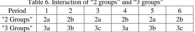
of products with 𝑘_𝑗 = 3. Table 6 (below) illustrates how each “2 group” is eventually paired with each “3 group”.

Table 6. Interaction of “2 groups” and “3 groups”

Period 1 2 3 4 5 6

"2 Groups" 2a 2b 2a 2b 2a 2b

Chapter 3

On the Lot Size Scheduling Problem, Part II: Determining Exact

Solutions to the ELSP under the Two and

Power-of-Primes Assumptions

Abstract: The Economic Lot Scheduling Problem (ELSP) is a classical scheduling problem with the objective of minimizing the long-run inventory and setup costs of a single machine, multi-product inventory system, subject to feasibility constraints. The problem is NP-hard (Hsu, 1983) and has been the subject of extensive study. The complexity of the problem has led to the use of various heuristics for restricted versions of the problem. Examples of classes of heuristics include basic period, power-of-two, and genetic

algorithms. This paper introduces a new method, the “power-of-primes,” and an algorithm which determines the optimal solution over all production schedules for both the power-of-two and power-of-prime methods. By optimizing over all production schedules, the results are guaranteed to be better than any heuristic under the same assumptions. The power-of-primes method is compared to Khouja et al.’s (1998) basic period genetic algorithm with favorable results. An experimental design is constructed which more accurately reflects problems commonly encountered in practice than Dobson’s (1987) design.

1 Introduction:

The Economic Lot Scheduling problem (ELSP) consists of a single machine assigned to

produce 𝑛 products. The machine is only capable of producing a single product at a time and requires a “setup time” before a product can be produced. The demand rate for product 𝑗 is

𝑑𝑗, the production rate 𝑝𝑗, and setup time 𝑠_𝑗 for 𝑗 = 1, …𝑛. Each time the machine is setup for product 𝑗 a cost of 𝑎_𝑗 is incurred. The unit cost of producing product 𝑗 is 𝑐_𝑗.

Additionally, there is an internal inventory cost rate 𝑖 proportional to the on-hand inventory. All parameters are assumed to be known constants and are independent of the order the

products are produced. The task is to find a cyclic (repeatable) production schedule which

minimizes long run inventory and setup costs while satisfying demand (stock outs are not

allowed). In the first of this 3-part series, a procedure was developed which proves the

optimality of the solution found by Haessler and Hogue (1976), and Doll and Whybark

The basic period approach assumes each production run of product 𝑗 has the same lot size (equal lot sizes) and each time product 𝑗 begins production the inventory of product 𝑗 is zero (zero-switch rule). The combination of equal lot sizes and the zero-switch rule imply

that the time between production runs of product 𝑗 is a fixed constant. The basic period approach assumes product 𝑗 is produced every 𝑘𝑗𝑇 units time where 𝑇 is a fixed positive constant independent of 𝑗, and𝑘_𝑗 is an integer. The variable 𝑇 is referred to as the “basic period” and the 𝑘_𝑗’s are referred to as the multipliers. This implies the lot size of product 𝑗 is

𝑑𝑗𝑘𝑗𝑇, the cycle time, 𝑡𝑗, is 𝑘𝑗𝑇, and the total variable cost for all 𝑛 products is

� �_𝑘𝑎_𝑗𝑇𝑗 +𝑖𝑐𝑗�𝑑𝑗𝑘₂𝑗𝑇� �1−_𝑝𝑗𝑑𝑗�� 𝑛

𝑗=1

. (1)

For a given 𝐤= [𝑘1⋯ 𝑘𝑛] and 𝑇, there is no guarantee a production schedule exists where

𝑑𝑗𝑘𝑗𝑇 product 𝑗 is produced every 𝑘𝑗𝑡 time units for 𝑗 = 1, … ,𝑛. Determining if such a

production schedule exists is NP-hard (Hsu, (1983)). If a production schedule does exist,

then (𝐤,𝑇) is said to be feasible.

The “power-of-two” method adds the constraint 𝑘_𝑗 = 2𝑧𝑗 _where 𝑧_{𝑗 is a non-negative}

integer. The motivation for the restriction is to aid in finding a production schedule for a

given 𝐤 and 𝑇. The “power-of-primes” method assumes that 𝑘_𝑗 is a power of a prime number in a set 𝑅. More formally, 𝑘_𝑗 =𝑟_𝑙𝑚𝑗 where 𝑟_𝑙 ∈ 𝑅 and 𝑚_𝑗 is a non-negative integer. The power-of-primes method includes the powers of 2, and the powers of 3, 5, 7, etc. Thus,

2 Literature Review:

The Economic Lot Scheduling Problem was first formally posed by Rogers (1958). Rogers

determined the optimal cycle time for each product and developed a heuristic to adjust lot

sizes and startup times to resolve any scheduling conflicts. Other early approaches include

the rotation cycle approach (Hanssmann (1962), Elion (1962)) and various “grouping”

procedures (Stankard and Gupta (1969), Hodgson (1970)).

The basic period approach discussed in the introduction originated with Bomberger

(1966). Bomberger provided a dynamic program which is effective for low to medium loads

and constructed a lower bound for the total cost of a cyclic schedule. Doll and Whybark

(1973) used an iterative method to determine the multipliers. Haessler and Hogue (1976)

developed a power-of-two version of Doll and Whybark’s work. Elmaghraby (1978)

provides a review of other earlier works.

Several later developments relevant to this paper include Hsu (1983), Dobson (1987),

Khouja et al. (1998), and Hanson et al. (2013). Hsu showed determining if a feasible

production schedule exists for a fixed (𝒌,𝑇) is hard (and, consequently, the ELSP is NP-hard). Dobson showed that every production sequence is feasible for some 𝑇> 0 provided

∑𝑛𝑖=1𝑑𝑖/𝑝𝑖 < 1 where 𝑑𝑖 is the demand rate for product 𝑖, 𝑝𝑖 is the production rate for

product 𝑖, and 𝑛 is the number of products being produced on the machine. Note that

∑𝑛𝑖=1𝑑𝑖/𝑝𝑖 is the proportion of time the machine must be in production (not including setup

time). Therefore, if ∑𝑛_𝑖=1𝑑𝑖/𝑝𝑖 ≥ 1 the machine does not have the capacity to meet demand. Additionally, Dobson introduced an unequal lot sizes scheduling heuristic.

Khouja et al. (1998) develop a genetic algorithm approach under the basic period

assumptions. For other genetic algorithms used to solve the ELSP see Raza and Akgunduz

(2008).

Hanson, et al (2013) considered the classical ten product ELSP data set introduced by

Bomberger (1966) under the basic period assumptions. A scalable depth-first search method

was used to determine all sets of multipliers 𝐤 which satisfy necessary feasibility conditions and have a cost less than the current best known solution (found independently by Doll and

remaining choices of 𝐤and conclude the solution found by Doll and Whybak, 1973 and Haessler and Hogue, 1976 is optimal under the basic period assumptions. To the best of the

authors’ knowledge, this is the first time a problem of any significant complexity has been

optimized over all production schedules.

The primary contribution of this paper is an algorithm which obtains exact solutions

under the power-of-two and power-of-prime assumptions. The algorithm is novel in that it

does not rely on a heurisitic to select the production schedule. Obtaining exact solutions over

all possible production sequences under the power-of-two and power-of-primes assumptions

is shown to obtain competitive solutions even in comparison to more relaxed assumptions

such as the basic period genetic algorithm of Khouja et al. (1998) and time-varying lot size

approaches (Dobson (1987), Raza and Akgunduz (2008), etc.) for parameters with values

reflective of those seen in practice.

3 Practical Motivation:

In practice, the production schedule is really a production “plan” which is modified to adjust

for slight fluctuations in demand, machine disruptions, approximation of parameters, etc.

According to Bomberger (1966), “Naturally, repetitive schedules that call for the same

quantity of an item to be made in each cycle cannot be strictly maintained in reality,” but “it

is often possible to adjust production to correct for such disturbances.” The cyclic schedule

“serves to guide the manager” and is a “workable first approximation.” This observation is

also made by Anderson (1990), who states “many companies that operate with production

period. The more complex unequal lot size schedules obtained by Dobson (1987) and

genetic algorithms (Raza and Akgunduz, 2008, etc.) may require more consideration when

making adjustments.

4 Methodology:

The following algorithm determines the minimum cost for the ELSP over all possible values

of 𝑇 and a set of power-of-prime multipliers. Typically, optimal lot sizes for products produced on the same machine have not been observed to deviate by more than a factor of

10. Throughout the remainder of the paper, the possible power-of-two multipliers will be 1,

2, 4, and 8, and of-prime multipliers will be 1, 2, 3, 4, 5, 7, 8, 9. Note that the

power-of-primes method allows for nearly all multipliers less than 10 (the only exception being 6).

The development is analogous for any choice of primes and multipliers.

The procedure to obtain the optimal solution for the power-of-two algorithm consists

of four main steps. First, the minimum cost of the rotation schedule is calculated and used to

determine an upper bound, 𝑇𝑚𝑎𝑥, and a lower bound, 𝑇𝑚𝑖𝑛, for the basic period, 𝑇. The range for 𝑇 is partitioned into intervals of width at most 𝛿 to condition on 𝑇 in the next step. The value of 𝛿 effects computational time, but all values of 𝛿 obtain the optimal solution. For this paper, 𝛿 = 1 is chosen.

Second, 𝑇 is assumed to be in the rightmost interval (i.e. [𝑇𝑚𝑎𝑥− 𝛿,𝑇𝑚𝑎𝑥]). All values of 𝐤with a potential lower cost than the current best solution (given 𝑇 is contained in the rightmost interval) are found using Hanson, et al (2013). Third, we determine if each 𝐤has a feasible production with a lower cost than the current best solution. If a lower cost is found,

the solution is updated. Fourth, steps two and three are repeated for each interval, from right

to left, until the entire range for 𝑇 has been searched.

1. Use the rotation (power-of-two) schedule to determine upper and lower bounds for 𝑇. Partition the range into sub-intervals of width at most 𝛿 > 0.

2. Determine all 𝐤which satisfy necessary feasibility conditions and have a potential lower total cost than the current best solution in the right-most sub-interval from (2)

3. For each 𝐤found in step 3, determine if a feasible production schedule exists with a lower cost.

4. Repeat steps 2-3 for each interval

The algorithm terminates with the optimal solution when the final sub-interval has been

considered. Sections 4.1, 4.2 summarize the relevant work from Hanson, et al (2013)

necessary to perform steps 1 and 2, respectively. Section 4.3 provides an efficient method to

determine if a feasible production schedule for a fixed (𝐤,𝐭) using a necessary and sufficient condition (Theorem 1), optimization results (Theorems 2,3,4), and “feasibility” tables.

The methodology is identical for power-of-primes, except that the initial solution is

the optimal power-of-two solution (instead of the rotation schedule).

4.1 Upper and Lower Bounds on the Basic Period (𝑻):

The initial feasible schedule to obtain the power-of-two schedule is the rotation schedule.

The optimal value of 𝑇 for the rotation schedule is the maximum of the global minimizer and the minimum time required for feasibility:

𝑇= max_�� 2 ∑𝑛𝑗=1𝑎𝑗

𝑖 ∑𝑛𝑗=1𝑐𝑗�1−𝑑𝑗_𝑝𝑗�𝑑𝑗

, ∑𝑛𝑗=1𝑠𝑗

1−∑𝑛𝑗=1(𝑑𝑗/𝑝𝑗)�. (2)

For the power-of-primes, the optimal power-of-two solution found by applying the algorithm

is used as an initial solution.

�2𝑑𝑗𝑎𝑗𝑖𝑐𝑗(1− 𝑑𝑗/𝑝𝑗) +�𝑀 − � �2𝑑𝑗𝑎𝑗𝑖𝑐𝑗�1−_𝑝𝑗𝑑𝑗� 𝑛

𝑗=1

� (4)

(See Hanson, et al (2013)). Note that this is a necessary but not sufficient condition. The

bound on variable cost can be used to find bounds on the cycle time using the quadratic

formula.

Figure 1: Total Cost vs. Cycle Time of Product 1 of the Bomberger Data

Let 𝑡_𝑗𝑚𝑎𝑥 and 𝑡_𝑗𝑚𝑖𝑛 denote the upper and lower bounds of 𝑡_𝑗, respectively. The cycle time of each product is at least the basic period (𝑡_𝑗 =𝑘_𝑗𝑇,𝑘𝑗 ≥1). Therefore, the basic period must be less than 𝑡_𝑗𝑚𝑎𝑥 for 𝑗 = 1, … ,𝑛. Additionally, the basic period must be long enough to setup and produce at least 𝑑𝑗𝑡_𝑗𝑚𝑖𝑛 product 𝑗 for all 𝑗. Let 𝑇𝑚𝑖𝑛 and 𝑇𝑚𝑎𝑥 denote upper and lower bounds of 𝑇. Then

𝑇𝑚𝑖𝑛 _{= max} 𝑗 �𝑠𝑗+

𝑡𝑗𝑚𝑖𝑛 𝑑𝑗

𝑝𝑗 � ≤ 𝑇 ≤min𝑗 �𝑡𝑗

𝑚𝑎𝑥_{�= 𝑇}𝑚𝑎𝑥_.

(5)

4.2 Determining all 𝒌 with a (potentially) lower cost given 𝒃 ≤ 𝑻 ≤ 𝒃+𝜹:

Consider the case where 𝑇 ∈[𝑏,𝑏+𝛿] for some fixed constant 𝑏. A method is required to determine all 𝐤 which have a potential lower cost than the current best solution given

𝑇 ∈[𝑏,𝑏+𝛿]. Recall the cycle time of product 𝑗, 𝑡_𝑗, is 𝑘_𝑗𝑇. The bounds for 𝑡_𝑗 and 𝑇from the previous section can be combined to find upper and lower bounds for 𝑘_𝑗. Let 𝑘_𝑗𝑚𝑖𝑛 and

𝑘𝑗𝑚𝑎𝑥 denote upper and lower bounds for 𝑘𝑗.

𝑘𝑗𝑚𝑖𝑛= �𝑡𝑗

𝑚𝑖𝑛

𝑇𝑚𝑎𝑥� and 𝑘𝑗𝑚𝑎𝑥 =�

𝑡_𝑗𝑚𝑎𝑥

𝑇𝑚𝑖𝑛� (6)

Hanson, et al (2013) re-index the products from the fewest possible multipliers to the most

(the number of possible multipliers is 𝑘_𝑗𝑚𝑎𝑥− 𝑘_𝑗𝑚𝑖𝑛+ 1). The depth-first search method conditions on 𝑘1. The minimum variable cost of product 1 given 𝑘1 =𝑙 where 𝑙 ∈

𝑘1𝑚𝑖𝑛, … ,𝑘1𝑚𝑎𝑥 and 𝑏 ≤ 𝑇 ≤ 𝑏+𝛿 is used to update the 𝑘𝑗𝑚𝑖𝑛 and 𝑘𝑗𝑚𝑎𝑥. If necessary

feasibility conditions are satisfied, the process conditions on 𝑘2. This process is repeated until either a 𝐤is found which satisfies the necessary feasibility conditions and has a potential cost less than the current solution or it is determined that no such 𝐤exists on that branch.

4.3 Determining the existence of a feasible production schedule given (𝒌,𝑇):

After searching an interval, a set of 𝐤’s is obtained which may have a lower cost than the current best solution. The uncertainty is due to the fact that, when the costs of the products

The total cost is found for the maximum of 𝑇∗ and Bomberger’s lower bound for 𝑇 to obtain the minimum cost of 𝐤 which may have a feasible production schedule. Denote the

maximum of 𝑇∗ and Bomberger’s lower bound by 𝑇_𝑙𝑏. If the cost is greater than the current best solution, then the value of 𝐤is disregarded and need not be reconsidered in future intervals.

If the cost is less, then a methodology is required to determine the minimum cost of a

feasible production schedule for 𝐤 over 𝑇. Subsections 4.3.1 and 4.3.2 develop a method to achieve this goal. Note that increasing the basic period of a feasible production schedule

preserves feasibility (provided ∑𝑛_𝑗=1𝑑_𝑗/𝑝_𝑗 < 1). The total cost equation can be solved for the largest value of 𝑇 which has a cost less than or equal to the current best solution. Denote this value of 𝑇 by 𝑇_𝑢𝑏. Feasibility is tested for 𝑇=𝑇_𝑢𝑏. If infeasible, then we conclude that no feasible production schedule with a cost less than the current solution exists for any value

of 𝑇 and 𝐤 is disregarded. If a feasible production schedule is found, then a feasible production schedule exists with a lower cost. In this case, 𝑇= 𝑇_𝑙𝑏 does not have a feasible production schedule and 𝑇=𝑇_𝑢𝑏 has a feasible production schedule. The smaller the value of 𝑇 on [𝑇𝑙𝑏,𝑇𝑢𝑏] the lower the total cost (as 𝑇∗ ≤ 𝑇_𝑙𝑏 and the total cost function is convex). Therefore, a one dimensional search over 𝑇 on the interval [𝑇𝑙𝑏,𝑇𝑢𝑏] to determine the

minimum value of 𝑇 which has a feasible production schedule will minimize total cost.

4.4 Mathematical Preliminaries:

If 𝐤 and 𝑇 are fixed, then the time required to setup and produce a lot of a product, 𝑗, is a fixed constant. Define 𝑡𝑗 =𝑠𝑗+𝑑𝑗𝑘𝑗𝑇/𝑝𝑗 to be the total setup and production time of product 𝑗 given 𝐤 and 𝑇. If the time required to setup and produce a product is greater than the basic period, then, clearly, there is no feasible production schedule. Without loss of

generality, assume 𝑡_𝑗 ≤ 𝑇 for all 𝑗 for the remainder of the section.

Note that a cyclic production schedule has a fixed number of basic periods. For

Lemma 1: A cyclic production schedule with 𝐤= [𝑘1⋯ 𝑘𝑛] has 𝑏= 𝑙𝑐𝑚(𝑘1, … ,𝑘𝑛) basic periods, where 𝑙𝑐𝑚(𝑘₁, … ,𝑘_𝑛) denotes the least common multiple of 𝑘₁,…,𝑘_𝑛.

Proof: Note the number of basic periods in a cyclic schedule is how often the schedule is repeated. Suppose that a cyclic schedule, 𝜃, repeats every 𝑧 basic periods. If the first production run of product 𝑗 in 𝜃 occurs in period 𝑓_𝑗, then product 𝑗 is produced in periods

𝑓𝑗+𝜆𝑘𝑗,𝜆= 1,2,3 …. The first production run of product 𝑗 in the second iteration of the

schedule occurs in period 𝑧+𝑓_𝑗. Therefore, 𝑧+𝑓_𝑗 = 𝑓_𝑗+𝜆_𝑗𝑘_𝑗 for some integer 𝜆_𝑗 for

𝑗 = 1, … ,𝑛. Thus, 𝑧= 𝜆₁𝑘₁ = 𝜆₂𝑘₂ = ⋯= 𝜆_𝑛𝑘_𝑛 for some 𝜆₁, … ,𝜆_𝑛 and 𝑧 is a common multiple of 𝑘1, … ,𝑘𝑛. Therefore, the first time the schedule is repeated is 𝑙𝑐𝑚(𝑘1, … ,𝑘𝑛) and

𝐤has 𝑙𝑐𝑚(𝑘₁, … ,𝑘_𝑛) basic periods. Q.E.D.

We now illustrate how the power-of-primes assumption aids in determining if a feasible

schedule exists. Consider 𝐤= [2 2 3 3 4] as a motivating example. Let 𝜌 be a production schedule satisfying 𝐤. The least common multiple of {2,2,3,3,4} is 12; so Lemma 1 implies

𝜌 has 12 basic periods.

Note that products 1, 2, and 5 have multipliers which are a power of 2 and products 3

and 4 have multipliers which are a power of 3. Let 𝜌₂ denote the sub-schedule of 𝜌

Table 1: Total Time by Period

Period 1 2 3 4 5 6 7 8 9 10 11 12

Prod.1,

2,5 𝑡21 𝑡22 𝑡23 𝑡24 𝑡21 𝑡22 𝑡23 𝑡24 𝑡21 𝑡22 𝑡23 𝑡24 Prod.

3,4 𝑡3

1 _𝑡

32 𝑡33 𝑡31 𝑡32 𝑡33 𝑡13 𝑡32 𝑡33 𝑡31 𝑡32 𝑡33

Total 𝑡21+𝑡31 𝑡22+𝑡32 𝑡23+𝑡33 𝑡24+𝑡31 𝑡21+𝑡32 𝑡22+𝑡33 𝑡23+𝑡31 𝑡24+𝑡32 𝑡21+𝑡33 𝑡22+𝑡31 𝑡23+𝑡32 𝑡24+𝑡33

Note that each 𝑡₂𝑥 is scheduled during the same period as each 𝑡₃𝑦 for 𝑥= 1,2,3,4 and

𝑦= 1,2,3 exactly once. Hanson, et al (2013) observed this will always be the case provided that the number of basic periods of the two sub-schedules are “relatively prime (i.e. they do

not share any common factors). Therefore, the production schedule is feasible if and only if

max{𝑡2𝑥|𝑥= 1,2,3,4} + max�𝑡3𝑦�𝑦 = 1,2,3� ≤ 𝑇 (7)

This result is generalized in Theorem 1.

Theorem 1: Let 𝜌 be a production schedule with multipliers 𝐤= [𝑘1⋯ 𝑘𝑛] and a fixed basic period 𝑇. Define 𝑅 = {𝑟₁, … ,𝑟_𝑣} to be a set of prime numbers and assume 𝑘_𝑗 = 𝜋𝑒𝑗 _for

some 𝜋 ∈ 𝑅, and 𝑒_𝑗 ∈ ℤ+. Let 𝜌_𝜋 be the sub-schedule of 𝜌 consisting of all products whose multiplier is a power of 𝜋 for 𝜋= 𝑟1, … ,𝑟_𝑣. The number of basic periods in 𝜌𝜋 is

𝑏𝜋 = max {𝑘𝑗|𝑘𝑗 =𝜋𝑒𝑗, 𝑗 = 1, … ,𝑛}. (8)

Therefore, the total time required to setup and produce the products scheduled by 𝜌_𝜋 rotates between 𝑏𝜋 values: 𝑡𝜋1, … ,𝑡_𝜋𝑏𝜋. Finally, define 𝜏𝜋 = max{𝑡𝜋𝑧|𝑧 ∈1, … ,𝑏𝜋}. The production schedule 𝜌 is feasible if and only if 𝜏1+⋯+𝜏𝑣 ≤ 𝑇.

Proof: We will show that 𝜏₁+⋯+𝜏_𝑣 ≤ 𝑇 implies 𝜌 is feasible. Note that each product is in exactly one sub-schedule. Therefore, the products scheduled for production in a basic

required to setup and produce all products scheduled by 𝜌_𝜋 is at most the maximum time 𝜏_𝜋, for 𝜋=𝑟₁, … ,𝑟_𝑣. Therefore, the time required to setup and produce every product scheduled by 𝜌 is at most 𝜏1+⋯+𝜏𝑣 and, as we assumed 𝜏1+⋯+𝜏𝑣 ≤ 𝑇, the production schedule 𝜌 is feasible.

It remains to be shown that 𝜌 is feasible implies 𝜏₁+⋯+𝜏_𝑣 ≤ 𝑇. Recall each sub-schedule, 𝜌𝜋, has 𝑏𝜋 basic periods. Define the 𝑏𝜋 basic periods of 𝜌𝜋 to be 𝜌𝜋1, … ,𝜌_𝜋𝑏𝑟 for

𝜋= 𝑟1, … ,𝑟𝑣. Without loss of generality, suppose 𝜌𝜋1 is scheduled for 𝜋= 𝑟1, … ,𝑟𝑣 in the

same basic period. By reasoning analogous to Lemma 1, the next time 𝜌𝑟1₁, … ,𝜌𝑟1_𝑣 will be scheduled in the same basic period is 𝑙𝑐𝑚(𝑏𝑟₁, … ,𝑏𝑟_𝑣). As each 𝑏𝜋 is the power of a distinct prime, 𝑙𝑐𝑚�𝑏_𝑟1, … ,𝑏_𝑟𝑣�=𝑏_𝑟1𝑏_𝑟2⋯ 𝑏_𝑟𝑣. Furthermore, there are only 𝑏_𝑟1𝑏_𝑟2⋯ 𝑏_𝑟𝑣 distinct ways to select one 𝜌_𝜋𝑦 for each 𝜋=𝑟1, … ,𝑟_𝑣, 𝑦 ∈1, … ,𝑏𝜋. Therefore, every combination of

𝜌_𝜋𝑦’s must occur exactly once before 𝜌_𝑟1₁, … ,𝜌_𝑟1_𝑣 is repeated: including 𝑡_𝜋𝑦 =𝜏_𝜋 for 𝜋 =

1, … ,𝑣. Therefore, as 𝜌 is feasible, 𝜏₁ +⋯+𝜏_𝑣 ≤ 𝑇. QED.

Define 𝑁𝜋 to be the set of all products whose multiplier is a power of a fixed prime 𝜋. Theorem 1 implies that feasibility can be determined by minimizing each 𝜏𝜋, the maximum total time required to setup and produce all products in 𝑁_𝜋 scheduled in the same basic period, over all production schedules with 𝐤= [𝑘1⋯ 𝑘𝑛] independently. Theorems 2, 3, and 4 are now presented to aid in the minimization of a given 𝜏_𝜋.

Theorem 2: Let 𝜋 be a prime number in 𝑅 and assume there are 𝜂 products in 𝑁_𝜋. Without loss of generality, assume products 1, … ,𝜂 are in 𝑁𝜋 and 𝑘1 ≤ 𝑘2 ≤ ⋯ ≤ 𝑘𝜂. If ∑𝜂_𝑗=11/

𝑘𝑗 ≤1, then 𝜏𝜋 = max�𝑡𝑗�𝑗 ∈1, … ,𝜂�.

Proof: Note 𝑘1 ≤ 𝑘2 ≤ ⋯ ≤ 𝑘𝜂 implies 𝑘𝜂 is the largest power of 𝜋 used as a multiplier. Therefore, 𝑙𝑐𝑚�𝑘₁, … ,𝑘_𝜂�=𝑘_𝜂 and Lemma 1 implies any production schedule for products

1, … ,𝜂 has exactly 𝑘_𝑛 basic periods. Recall product 𝑗 is produced every 𝑘_𝑗 periods.

Therefore, product 𝑗 is produced 𝑘_𝑛/𝑘_𝑗 times in a production schedule and the total number of production runs over products 1, … ,𝜂 is ∑𝜂_𝑗=1𝑘_𝜂/𝑘_𝑗. Thus, the number of production runs is less than or equal to the number of basic periods if and only if

�𝑘𝜂_𝑘 𝑗 𝜂

𝑗=1

≤ 𝑘𝜂 or �_𝑘𝑗1 𝜂

𝑗=1

≤1. (10)

The first production run of each product determines the production schedule. If the first

production runs are assigned, in order from product 1 to product 𝜂, to the first available basic period, then each production run is in a distinct period. Q.E.D.

Consider the case where only one power, 𝛼, of a specific prime, 𝜋, is used as a multiplier. By Theorem 2, if the number of products in 𝑁_𝜋 is less than or equal to 𝜋𝛼, then

𝜏𝜋 = max�𝑡𝑗�𝑘𝑗 = 𝜋𝛼�. (11)

A closed form solution for 𝜏_𝜋 is now determined for the case where the number of products in 𝑁_𝜋 is 𝜋𝛼+ 1.

Theorem 3: Let 𝜋 be a prime number in 𝑅 and assume there are 𝜂 = 𝜋𝛼+ 1 products in 𝑁𝜋. Without loss of generality, assume products 1, … ,𝜂 are in 𝑁𝜋 and 𝑡1 ≤ 𝑡2 ≤ ⋯ ≤ 𝑡𝜂.

Assume 𝑘_𝑗 = 𝜋𝛼 for 𝑗 = 1, … ,𝜂. Then 𝜏_𝜋 = max�𝑡₁+𝑡₂,𝑡_𝜂�.

time required to produce two products is 𝑡1+𝑡2. Furthermore, 𝑡𝜂 appears in some basic period. Therefore, 𝜏𝜋 ≥ max {𝑡1+𝑡2,𝑡𝜂}. Any production schedule where products 1 and 2 are scheduled in the same period and all other products are scheduled in a distinct periods

will obtain 𝜏_𝜋 = max�𝑡₁+𝑡₂,𝑡_𝜂�. Q.E.D.

Without loss of generality, assume products 1, … ,𝜂 are in 𝑁_𝜋 and define 𝐤_𝜋 = [𝑘₁⋯ 𝑘_𝜂],

𝑘1 ≤ 𝑘2 ≤ ⋯ ≤ 𝑘𝜂 and 𝐭𝜋 = [𝑡1⋯ 𝑡𝜂]. For some values of (𝐤𝜋,𝐭𝜋) it is possible to define

an equivalent problem, (𝐤_𝜋′,𝐭_𝜋′), which has the same value of 𝜏_𝜋 as (𝐤_𝜋,𝐭_𝜋). If 𝜏_𝜋 has already been found for (𝐤𝜋′,𝐭𝜋′), then there is no need to solve 𝜏𝜋 for (𝐤𝜋,𝐭𝜋). An illustrative example is provided below.

Let 𝐤_𝜋 = [2 2 4 8],𝐭_𝜋 = [𝑡₁ 𝑡₂𝑡₃ 𝑡₄], and 𝜃 be an arbitrary production schedule for products 1, 2, and 3. Note 𝜃 has four basic periods and product 4 is produced every eight periods. Therefore, product 4 is scheduled every other iteration of 𝜃. The maximum time required to setup and produce each product scheduled during a basic period (𝜏₂) clearly occurs during an iteration of 𝜃 with product 4 (as it is the same production schedule, plus an additional product). Therefore, theoretically, if product four is produced in every iteration of 𝜽 (but with the same value for 𝒕𝟒), then the value of 𝜏2 will be the same. Thus, 𝐤𝜋 =

[2 2 4 8],𝐭𝜋 = [𝑡1 𝑡2𝑡3 𝑡4] and 𝐤𝜋′ = [2 2 4 4],𝐭𝜋′ = [𝑡1 𝑡2𝑡3 𝑡4] have the same value of 𝜏2.

Alternatively, a fifth product with, 𝑘₅ = 8, 𝑡₅ ≤ 𝑡₄, could be added without changing

𝐤𝜋, respectively. Let 𝑀 be the number of products with 𝑘𝑗 =𝑚1. If 𝑀 ≤ 𝑚1/𝑚2, then 𝜏𝜋 is the same for (𝐤_𝜋,𝐭_𝜋) and 𝐤_𝜋′ = [𝑘₁, … ,𝑘_𝜂−𝑀,𝑚₂], 𝐭_𝜋′ = �𝑡₁, … ,𝑡_𝜂−𝑀, max�𝑡_{𝜂−𝑀+1}, … ,𝑡_𝜂��.

Proof: Observe the first 𝜂 − 𝑀 products in (𝐤𝜋,𝐭𝜋) and (𝐤𝜋′,𝐭𝜋′) are identical. Let 𝜃 be an arbitrary production schedule for products 1, … ,𝜂 − 𝑀. The final product in 𝐤_𝜋′, 𝜂 − 𝑀+ 1, has a multiplier of 𝑚2 and its total setup and production time is max�𝑡𝜂−𝑀+1, … ,𝑡𝜂�. Let 𝑗∗ be a product in 𝐤_𝜋 such that 𝑡_𝑗∗ = max�𝑡_{𝜂−𝑀+1}, … ,𝑡_𝜂� and 𝑘_𝑗∗ =𝑚₁. Note product 𝜂 − 𝑀+

1 in 𝐤_𝜋′ and product 𝑗∗ in 𝐤_𝜋 have the same total setup and production time. Therefore, scheduling 𝜂 − 𝑀+ 1 in 𝐤𝜋′ or 𝑗∗ in 𝐤𝜋 in the same basic period of 𝜃 will result in the same

𝜏𝜋. Note, product 𝑗∗ in 𝐤𝜋 will appear in fewer iterations of 𝜃, but this does not alter 𝜏𝜋.

Furthermore, each of the remaining products in 𝐤_𝜋 with a multiplier of 𝑚₁ can be scheduled in 𝑗∗’s place in the remaining 𝑚1/𝑚2−1 iterations of 𝜃 without altering 𝜏𝜋. Q.E.D.

Theorems 1-4 provide methods to quickly determine the feasibility of (𝐤,𝐭) for many values of 𝐤 and 𝐭. To illustrate, consider the following example: 𝐤= [1 2 2 3 3 3 4], 𝐭=

[5 4 2 2 3 3 3], and 𝑇= 15. Product 1 is produced in every period. Therefore, we subtract

𝑡1 from 𝑇 and obtain 𝐤′= [2 2 3 3 3 4], 𝐭′ = [4 2 2 3 3 3], 𝑇′= 10.

By Theorem 1, (𝐤′,𝐭′) is feasible if and only if 𝜏₂+𝜏₃ ≤ 10. Note 𝑁₂ = {1′, 5′, 6′} and 𝑁3 = {3′, 4′, 5′}. Theorem 4 implies [2 2 4] has the same value of 𝜏2 as [2 2 2] with the same production times. Theorem 3 implies 𝜏₂ for [2 2 2] is max{𝑡₁′ +𝑡₂′,𝑡₃′} where 𝑡₁′ ≤

𝑡2′ ≤ 𝑡3′ are the production times of the three products. Therefore, 𝜏2 = max{2 + 3,4} = 5.

Consider 𝑁₃. As 1/𝑘₃′ + 1/𝑘₄′ + 1/𝑘₅′ = 1/3 + 1/3 + 1/3≤ 1, Theorem 2 implies 𝜏3 = max{2,2,3} = 3. Therefore, 𝜏2 +𝜏3 = 8 < 10 and we conclude a feasible schedule exists for 𝐤= [1 2 2 3 3 3 4], 𝐭= [5 4 2 2 3 3 3], and 𝑇= 15. Note that there is no benefit to constructing the actual schedule during the implementation of the algorithm.