Effect of Lighting Variability on the Color Difference Assessment

Abstract

Noor, Kashif. Effect of lighting variability on the color difference assessment (under the supervision of Dr. David Hinks.)

The purpose of this study was twofold: a) to quantify the degree of lighting variability in selected large and medium retail stores, and to compare the measured area lighting to the quality of lights used in selected standard light booths, and b) to assess the performance of the current ISO and AATCC recommended color

difference formula, DECMC, to a new formula, CIEDE2000 (or DE00), recently recommended by the Commission Illumination de l’Eclairage (CIE).

The effect of lighting variability was assessed using two pairs of metameric dyed cotton samples. Spectroradiometric measurements of several large

department stores were taken at various locations around the store, including areas in which clothing was displayed, changing areas, in front of full length mirrors, at the check-out counter, etc. Similar measurements were made at several medium sized retail chain stores. The lighting variability was assessed using key factors, including illuminance (lx), correlated color temperature, metamerism index and color

inconstancy index. Using the measured spectral data at each location in the store, and the reflectance factors of the two metameric pairs, the variability in key

colorimetric data was calculated and compared to standard illuminant data. Also, as a new color difference formula has been recently adopted by the CIE, the

pairs (100% polyester) around 5 color centers. The colors of four of the color centers were selected to be in regions of color space that the new formula is

reported to perform better than DECMC, namely blues, dark, and near neutral colors. The performance of each color difference formula was assessed against visual pass/fail data for thirty one expert shade matchers were using each color difference pair.

Considerable variability was found within each store measured, and between stores, for each of the colorimetric and radiometric variables studied. For instance, the illumination levels varied from 50 Lux to approximately 1800 Lux and very often did not comply with the levels recommended by the Illuminating Engineering Society (IES). DEcmc values ranged from .4 to 7.5. In general, the lighting variability at the point-of-sale indicates strongly that protocols for selecting dye recipes should be developed to minimize color inconstancy between the light sources used in the store in order to insure that the color perceived by the consumer is close to that intended by the product designer.

Effect of Lighting Variability on the Color Difference Assessment

By Kashif Noor

A thesis submitted to the Graduate Faculty of North Carolina State University

In partial fulfillment of the Requirements for the

Degree of Master’s of Science in

Textile Chemistry

Raleigh 2003 Approved By:

Dr. David Hinks Dr. Brent C. Smith (Chair of Advisory Committee)

Biography

Kashif Noor was born on September 28, 1977 in Toba Tek Singh, Pakistan. He started his elementary education in Bern (Switzlerland) and completed

Primary School in Pakistan, he was in Kuwait City for Middle School and finished his High School from Tehran.. He got his Bachelors in Textile Engineering with concentration in Dyeing & Finishing Operations from the University of

Acknowledgement

The author would like to extend his gratitude to Dr. David Hinks, Chairman of Advisory Chairman of his advisory committee, for his advice and guidance throughout this study. It was his confidence in the author and continuous encouragement that made this work possible. Appreciation is also extended to

the other members of the committee, Dr. Brent Smith and Dr. Warren Jasper for the valuable advice.

The author would also like to thank Jeff Krausse for his help with the dyeing of samples. Dr. Timothy Clapp for his help and assistance in the statistical analysis of the data, this helped to quantify the data in a meaningful way.

Finally, the author is extremely grateful to his parents for all their love and

Table of Contents

List of Tables ……… x

List of Figures ……….. xi

1. Radiometry……… 1

1.1 Electromagnetic Spectrum……… 1

1.2 Light……… 1

1.3 Measurement of Light ……….. ……….. 3

1.3.1 Radiance Flux (ФЄ)………. 3

1.3.2 Luminous flux (Фv)……… 3

1.3.3 Luminous Efficacy………. 4

1.3.4 Steradian angle……… 4

1.3.5 Radiant and luminous intensity (I)……… 5

1.3.6 Irradiance and illuminance(lux)……… 5

1.3.7 Radiance and luminance (L) ……… 6

1.3.8Troland……… 6

1.4 Black Body Radiation……… 7

1.5 Mechanisms by which radiation is produced……… 8

1.5.1 Incandescent……… ……….. 8

1.5.2 Electric Discharge Lamps……… … 8

1.5.2.1Sodium and Mercury Vapor Lamps………. 8

1.5.2.2 Fluorescent lamps………. 9

1.5.3 Xenon Arc Lamps ………. 10

1.6 Color Temperature………. 10

1.7 Correlated Color Temperature……… 11

1.8 Lamp Efficacy………. 11

1.9 Color Rendering Index ……….. 12

1.10 Spectroradiometry ……….. 12

1.10.1 Monochromator……….. 13

1.10.2 Polychromator ……… 14

2. Color Space and Color Order Systems………15

2.1 Tristimulus Values……….. 15

2.2 The Chromaticity Diagram ……….16

2.3 Color Order-Systems………. 18

2.4 CIE Lab Color Space ………. 18

2.5 Single Number Pass/Fail Criteria……… ……….19

2.5.1 CIELab color difference formula……….. 20

2.5.2 The JPC79 color difference formula ……… …21

2.5.3 CMC (l: c) Color Difference Formula ……… 22

2.5.4 BFD (l: c) Color Difference Equation……… 24

2.5.5 CIEDE2000 (kL: kC: kH) color difference formula ……….24

2.6 Color Perception Phenomena……….28

2.6.1 Color Incontancy……… 28

2.6.2.1 Illuminant metamerism ……….. 29

2.6.2.2 Observer metamerism……….. . 30

2.6.2.3 Field Size metamerism……… ………. 30

2.6.2.4 Geometric metamersim ………. 30

3. Retail Lighting……….. 31

3.1 Lighting design ……… 31

3.1.1. Lamp selection……… 31

3.1.2 Luminaire……… 32

3.1.3 Light diffusing methods………. 32

3.1.4 Lighting Variability……… 33

3.1.4.1 Light Loss and non-uniformity factors……….. 24

3.1.5 General Considerations for illuminance ………. 35

3.1.6 Factors affecting an observer’s visual comfort in retail store . 36

3.1.6.1 Psychological factors ………. 37

4. Research Proposal ………. 38

I.Experimental ……… 40

1. Equipment ……… ….. 40

2. Retail Store measurements ………. 40

2.1 Data Evaluation ……….. 42

3. Light Box Measurements ………. 43

5. Comparison of the performance of CIEDE2000 and DEcmc via visual

assessment ……….45

6. Performance of CIEDE2000 and DEcmc under different illuminants 49

II. Results and Discussion………. 50

1. Metameric pairs ……… 50

2. Light box measurements……….51

3. Measurement of stores ………52

3.1 Store A………. 52

3.2 Store B ……….56

3.3 Store C ……… .59

3.4 Store D………. 62

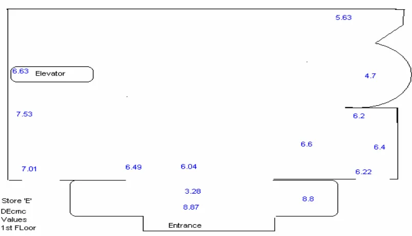
3.5 Store E ……….65

3.6 Store F………. 68

3.7 Store G ……….. 70

3.8 Comparison of photometric and colorimetric data between stores 73

3.8.1 Check-out counters ……… 73

3.8.2 Statistical Analysis……… .75

3.8.2.1 Color Difference (DEcmc (2:1)) ……….. ……….76

3.8.2.2 Color Inconstancy……… 77

4. Comparison of the performance of CIEDE2000 and DECMC by visual

assessment………. 79

5. Analysis of variation in CIEDE2000 and DEcmc as a function of illuminant ……… 88

5.1 Variation as a function of hue angle, ho ………89

IV. SUMMARY AND CONCLUSIONS ………. 99

1. Lighting variability in retail stores………... 99

2. Performance of DECMC and DE00 against a new visual dataset………... 100

3. Analysis of variation in CIEDE2000 and DEcmc as a function of illuminant ………. 101

V. REFERENCES ……….. 102

VI. APPENDIX ………. 107

Table VI.1 Standard deviation, mean and confidence intervals for DEcmc (2:1) 107

Table VI.2 Wilcoxon / Kruskal-Wallis Tests (Rank Sums) for DEcmc (2:1) …… 107

Table VI.3 One way Test, ChiSquare Approximation for DEcmc (2:1) ………… 107

Table VI.4 Standard deviation, mean and confidence intervals for Color Inconstancy ………. 107

Table VI.5 Wilcoxon / Kruskal-Wallis Tests (Rank Sums) for color inconstancy ……… 108

Table VI.6 One way Test, ChiSquare Approximation………. 108

Table VI.8 Wilcoxon / Kruskal-Wallis Tests (Rank Sums) for Color Rendering Indices. ……….109 Figure VI.9 One-Way Analysis of Color Rendering Index……… 109 Table VI.10 Standard deviation, mean and confidence intervals for CCT ……110 Table VI.11 One way Test, ChiSquare Approximation……… …… 110

List of Tables

Table1. Colorimetric data of color centers (CIELAB, D65/10o observer) ………..47 Table2. Colorimetric data of sample pairs (CIELAB, D65/10o observer) ………..48 Table 3. Colorimetric data for the standard and the trial metamers ……….50 Table 4. Summary of colorimetric data for turquoise metamers

using SPD data of standard light booths. ………... 52 Table 5. Observer Pass/Fail Data versus ∆ECMC & ∆E00 ……… 83 Table 6. Summary of symbols used in discrimination equation 1. ………..84 Table 7. Distribution of samples under different illuminants

through out the hue region ……….. ……….... 89 Table 8. Comparison of arithmetic mean of color difference data

for all samples across entire hue range……… 93 Table 9. The predicted range of difference by Wilcoxon Test based

for each hue name. ……… 96 Table 10. Colorimetric data for blue samples with hue angle in

List of Figures

Figure1. Electromagnetic Spectrum ………1 Figure2. How Illuminance is defined……….. 5 Figure3. Schematic diagram of a monochromatic spectroradiometer ………….13 Figure4. CIE 1931 Chromaticity Diagram ……….16 Figure 5. Plot of CIE L*a*b* space………... 19 Figure 6. Reflectance spectrum of the standard and the trial ……… ..50

Figure 17. DECMC data calculated for blue metamers using SPD data and blue metamers for Store C……… 60 Figure 18. Color inconstancy index for standard blue metamer for store C…. 61 Figure 19. Illuminance values for the various locations of store C……… 61 Figure 19. Normalized spectral power distribution data for measurements

taken at store ………. 62 Figure 20. Normalized spectral power distribution data for measurements

taken at store ..……….. 62 Figure 21. Normalized spectral power distribution data for measurements

taken at store D near the external windows

(measurements taken during the day).. ………..63 Figure 22. DECMC data calculated for blue metamers using SPD data

and blue metamers for Store D.……….... 63 Figure 23. Color inconstancy index values for standard blue metamer

for store D ……….. 64 Figure 24. Illuminance values for the various locations of store D 64

Figure 25. Normalized spectral power distribution data for

measurements taken at store E………. 65 Figure 26. DECMC data calculated for blue metamers using SPD

data and blue metamers for Store E. ………. 66 Figure 27. Color inconstancy index values for standard blue

Figure 29. Normalized spectral power distribution data for

measurements taken at store F. ……….. 68 Figure 30. DECMC data calculated for blue metamers using

SPD data and blue metamers for Store F. ………. 69 Figure 31. Color inconstancy index values for standard blue

metamer for store F ……….. 69 Figure 32. Illuminance values for the various locations of store F……….. 70 Figure 33. Normalized spectral power distribution data for

measurements taken at store G………... 70 Figure 34. DECMC data calculated for blue metamers using SPD data and blue metamers for Store G………. 71 Figure 35. Color inconstancy index values for standard blue

metamer for Store G ……… 72 Figure 36. Illuminance values for the various locations of Store G………… . 72 Figure 37. DEcmc values at the check out counters in different stores. … 74

Figure 38. Comparison of illuminance (lx) values at the check-out

counters in the six stores studied……… 74 Figure 39. Comparison of metamerism index (M.I.) and

color inconstancy index (C.I.) values at check-out counters in the six stores studied ………. 75 Figure 40. Comparison of CIE color rendering index C.R.I values

Figure 41. Comparison deviation among light booths with deviation among the retail

stores using one way analysis of DEcmc………... 77

Figure 42. Comparison deviation among light booths with deviation among the retail stores using one way analysis of color Inconstancy Index ………78

Figure 43. Comparison deviation among light booths with deviation among the retail stores using one way analysis ofmetamerism index………. 79

Figure 44. Percent discrimination for ∆ECMC(2:1) ∆E00(2:1) and CIELAB ∆E at three pass/fail values ………. 85

Figure 45. Percent discrimination for ∆ECMC(1:1) ∆E00(1:1) and CIELAB E at three pass/fail values. ……….86

Figure 46. Calculated values of DECMC (solid) and DE00 (dashed) plotted against ho for D65………. 90

Figure 47. Plot of DECMC - DE00 against ho _{and C* for D65……… 91}

Figure 48. Plot of DECMC - DE00 against ho and C* for illuminant A. ……… 92

1. Radiometry

1.1 Electromagnetic Spectrum

Electromagnetic radiation is one type of several forms of energy. The prime source for the radiation is from the sun and the cosmic rays entering the atmosphere. The spectrum is made up of different levels of radiation varying in frequency and

wavelength consisting of UV, infra-red, visible light, γ-rays, etc. Radiation can also

be produced by oscillating electrical circuits, which can range from several thousand meters to less than a millimeter. The visible spectrum is comprises only a small region of the electromagnetic spectrum as indicated in the diagram below:

X-rays Visible Microwave

Gamma rays UV IR Radio Waves

10-11 10-9 10-7 10-5 10-3 10-1 10 103

Wave Length (cm)

Figure 1. Simplified diagram of the electromagnetic spectrum.

1.2. Light

Electromagnetic radiation travels in the form of a transverse wave and can be

characterized by wavelength and frequency2. The number of waves passing through one point in one second will be the frequency denoted by ν, and it can also be given as the reciprocal of time, t,

The propagation of light can be well explained by the electromagnetic theory of light but fails to explain the emission and absorption of light. The exchange between the light and matter takes place in discontinuous process as compared to continuous process proposed by earlier theories. Max Plank (1905) demonstrated this exchange of energy takes place in form of quanta. The total amount of energy is given by Є = h. ν (2) where v is the frequency of the radiation and h is a constant (h = 6.624 x 10-27 erg. sec). The idea of continuity in waves has been discarded because the kinetic translation of energy takes place in jumps. According to Einstein’s law3 _{(1905), the} quantum energy (hν) is equal to the sum of energy WO, to free the electron from the atom of the metal surface and W (kinetic energy) of the electron outside the atom. WO + W = hν (3)

The wavelength in terms of quantum energy can be given by

Є = 1240 / λ electron-volts (4)

In 1924, through Louis De Broglie’s work, a relationship was recognized between waves and photons. Wave mechanics has been able to explain the wave-particle duality of light.

Whenever light travels through a medium of refractive index η, the speed of the light is altered according to the following relationship:

Speed of light in a medium = c

/

1.3. Measurement of Light

Radiometric measurements refer to the energy of the radiation while photometric measurements are weighted by the visual sensitivity (the so-called Vf function) of the average visual observer at 555 nm. A point source is one which produces its own radiation and is the same in all directions. A Lambertian source is one in which light travels through a transparent medium and is highly diffuse or is reflected from a surface.

1.3.1 Radiance Flux (ФЄ)

Radiance flux (ФЄ) is the energyper unit time (dQ/dt) that is radiated from a source with the range of .01 to 1000 µm4, which includes the visible, infra-red and U.V regions. A radiant flux of 1 watt means that the source produces 1 joule of energy per second.

1.3.5 Luminous flux (Фv)

1 lumen= radiant power x 1/683 watt x luminous efficacy (6)

From quantum mechanics5, photon energy at 555 nm Є = hν = 3.582 x10-15 _{J (7)}

and 1 lumen = 1.464x10-3 J/s (8)

N = 1.464x10-3 /3.582 x10-15 (9)

1 lumen = 1.4087 x 1015 _{photons/second}5 ₍₁₀₎

1.3.3 Luminous efficacy Luminous efficacy is defined as the ratio of photometric flux to the total radiometric flux: K = Фv /ФЄ (11)

1.3.4 Steradian angle

The steradian is the SI unit of solid angular measure. A steradian is conical in shape and has a unit of 1 if the subtended ‘area’ is equal to the square root of radius.

Radius = I unit Area = I square unit

The numerical value of solid angle, Ω, is given by:

Ω = A / r2 (12) 1.3.5 Radiant and luminous intensity (I)

The radiant and luminous flux per unit solid angle is called as radiant and luminous intensity, respectively. For luminous intensity we will get:

I = dФ/dω ( candela) (13)

Hence, candela is defined as the luminous intensity in a given direction of a source that emits a monochromatic radiation of frequency 540 x 1012 Hz and that has a radiant intensity in that direction of 1/683 watt per steradian. Hence, by this measure intensity falls as the distance increases by square of the distance and is called as inverse square law

1.3.6 Irradiance and illuminance (lx)

Irradiance is the measure of radiant flux per unit area (W/m2), whereas illuminance is the measure of luminous flux per unit area, as shown in Figure 2.

_{Foot-candle = lm / ft}2

1 meter

1 foot Lux

1 lm/m2

1 f.c 1lm/ft2 _1Sr

Irradiance from an extended source is related to the radiance of the source by the following equation:

E = π L sin2 (θ/2) (14) This shows that the irradiance primarily depends on the central angle of viewing of the detector.

1.3.7 Radiance and luminance (L)

Both radiance and luminance can be defined as the flux density per unit solid angle. Radiance is independent of distance for an extended area source, because the sampled area increases with distance, canceling inverse square losses.

Luminance = 1 lm/m2_{/sr or (15)} Candela / m2

1.3.8 Troland

A troland is the “unit of retinal illuminance equal to that produced by viewing a surface having a luminance of 1 candle per square meter through a pupil having an area of 1 square millimeter” 34

1.4 Black Body Radiation

but this is a very small factor which does not really contribute significantly to the black body radiation curve6. In 1879, Josef Stefan showed that the radiation emitted is independent of the material. The black body radiation curves obtained by Max Plank were the advent of quantum theory, because the mathematical derivation assumes that energy is in discrete packets called quanta. The curves obtained are called black body (or Plankian) curves since they represents an idealized body that does not reflect or transmit light. The Plankian equation used is shown below: Me = c1 (16) λ5[exp (c2/λΤ) -1]

where,

Me = emittance per wave length interval (Wm-3) T = absolute temperature if the source (Κ)

λ = wave length of the radiation band (m)

c1 = 3.74 x 10-16 Wm-2 c2 =0

1.5 Mechanisms by which radiation is produced

1.10.1 Incandescent

energy emitted by an incandescent solid is less than the black body at the same temperature. Emissitivity (ε) is the ratio of radiant excitance. This part is heated

again and the emitted photon might have a higher or lower energy7.The energy emitted by the incandescent radiator to that of the black body. The emissivity of tungsten is not quite constant but decreases with increase in wavelength.

Characteristics:

Light of different wavelengths is emitted from different parts of the filament. When a part of the filament emits photons, it looses energy in the process and cools down.

1.5.2 Electric Discharge Lamps

When an electric current is passed through a gas or vapor, gas molecules get excited by the collision with the electrons. When the electrons come back to their normal state, they will emit radiation. They emit line spectrum instead of continuous spectrum by incandescent lamps.

Following are a few kinds of discharge lamps.

1.5.2.1 Sodium and Mercury Vapor Lamps

the temperature and pressure in the presence of aluminum oxide tubes. Mercury lamps exhibit a bluish color to the light they emit. One half of the radiant power emitted is in the ultraviolet region and by coating the inside of the lamps by phosphors can convert this U.V part into visible region. These lamps are very

efficient in converting electrical power into energy and thus being widely used for out door lighting. The kinetic energy of the electrons produced in the low pressure

discharge is characterized by Maxwell-Boltzmann function:

F (Є) dЄ = 2π x Є1/2 exp (-Є/ ΚBT) Dє (17) πΚB T1/2

1.5.2.2 Fluorescent lamps

In the presence of mercury liquid and a rare gas, radiation is produced which is rich in U.V content. With the help of different phosphors, different kinds of spectral power distribution can be obtained. Calcium tungstate can be used as a phosphor for cool fluorescent lighting with lead as an activator to improve the efficiency of the

1.5.3 Xenon Arc Lamps

A high voltage pulse is used to ionize a high pressure xenon gas which produces a continuous spectrum over the U.V and visible region except for line emission at 450 nm and 500 nm. At low pressure, a bluish-green hue is obtained with a greater number of line emissions at the lower wavelength.

The line emission can be controlled by varying the intensity of the applied current and the vapor pressure. This lamp is currently used for light fastness tests and as a day light simulator by measuring instruments like spectrophotometers.

1.5.4 Lasers

A coherent and monochromatic radiant energy of high intensity is obtained by the Laser (light amplification of stimulated radiation).Its a process in which an excited molecule is striked by a photon. They can in a range of a few milliwatts to hundreds of kilowatts. Lasers are extremely important as monochromators and for aligning optical instruments.

6. Color Temperature

Log P = ao – 11350 / Tc (18) where ao is a constant depending on the size of the filament

7. Correlated Color Temperature

It is the temperature of the Plankian radiator whose perceived color resembles that of a given stimulus under the same brightness and specific conditions.

However, suggestions have been made to change the above definition as follows: “The temperature of Plankian radiator whose chromaticity is the nearest to the chromaticity of the given stimulus on a diagram where the CIE 1931 standard observer based on u’, 2/3v’ co-ordinates of the Plankian locus and the test stimulus are depicted” 9.

8. Lamp Efficacy

Human observer is very sensitive to the light at 555 nm (yellow-green) as compared to blue and red which appear dimmer even if they are of the same radiant flux. The term photopic curve describes the sensitivity of the eye to the radiation through out the visible spectrum. The total luminous flux F, can be calculated from

F = Κm∫ Pλ Vλdλ (19) Where Pλ is the radiant flux and Κm is the luminous efficacy

9. Color Rendering Index

different and the sample may reflect different wave lengths and look different. Most of the lamps developed today emit light that is concentrated at three or four wave lengths having a higher lamp efficacy and a source which has a broader spectrum usually has good color rendering properties and lower lamp efficacy. Plankian radiator is used as a reference for lamps with CCT less than 5000K; and Illuminant D where the CCT is greater than 5000K.

Incandescent lighting has been a source of lighting for quite some time now..

Fluorescent lighting has a higher lamp efficacy and longer lamp life but initial cost is high. Some problems might be seen in textiles under this lighting due to the

presence of FBA’s. Color rendering index can be measured by either by CIE special color rendering index

Ri = 100 – 4.6di (20) The CIE general color rendering index is given by

Ra = 100 – [4.6/8 x (d1 + d2+…..d8)] (21) where di is the distance in the CIE U*V*U* between color coordinates of the test source and the nearest D source and d1 to d8 are the Ri values for the Munsell color circle at value 6.

10. Spectroradiometry

A spectroradiometer measures radiometric quantities as a function of wavelength. Following characteristics can be known through the instrument:

I. Spectral Power Distribution

IV. Correlated Color Temperature V. Luminance, illuminance etc

i. Monochromator

The radiation enters the monochromator where it is dispersed and transmitted via a narrow band of wavelengths through the exit slit which connected to the detector. Photoelectric response by the detector takes place which is analyzed by the computer. The measurement of the spectral radiometric quantity also involves the comparison of the test source with a reference source whose spectral power distribution is known. The wave length band transmitted by the monochromator is the same as used in the calculation of the tristimulus vales. F

Figure3. Schematic diagram of a monochromatic spectroradiometer

A = Optical Coupler B = Electronic Interface C = Reference Source D = Test Source

c

A

D

Monochromator

A

B Computer B

B

Display

E = Detector

F = Power supply and measuring instrument

ii. Polychromator

In this case the dispersion of spectral power is done by a polychromator. It

measures the flux at wavelengths at the same time which is done by the dispersing element onto a silicon detector. An array of 256 elements is spread out uniformly over the visible region. Such instruments can take a measure in fraction of a second but the accuracy is compromised because of the poor signal to noise ratio of the silicon detector.

The selection of the wavelength interval depends on the complexity of radiant power. For, incandescent light an interval of 10 nm will be sufficient because of the

2. Color Space and Color Order Systems

2.1 Tristimulus values

The colors of objects are specified by the CIE according to a numerical theory based on trichromacy theory35 . Color specification necessarily requires specification of the light source spectral power distribution, S, reflectance spectrum of the object, and the response of the eye of the observer, known as color matching functions. The CIE has defined two standard observers: the 2 degree standard observer and the 10 degree supplemental standard observer36.

Owing to the presence of three receptors in the eye [ref] for the average color

normal observer, three numbers are required to define the color matching functions. Hence, three numbers are required to specify any object color according to the equations shown below. XYZ are known as tristimulus values.

X =

∑

. .R

S x (22)

Y =

∑

. .R

S y (23)

Z =

∑

. .R

S z (24)

Where

S = Spectral Power Distribution.

R = Reflactance ( or Transmittance) of sample.

2.2 The chromaticity diagram

A convenient way to represent the tristimulus values of object colors in a

mathematical space is by using a two dimensional scale, known as chromaticity coordinates, defined according to the relationship:

x = X / X + Y + Z (25) y = Y / X + Y + Z (26)

z = Z / X + Y + Z (27)

From the above equations we know that x + y + z = 1, so if we know any two of the variables the third can be found out.

0 .3 .6 .9 x

Figure 4. The CIE 1931 chromaticity diagram. H

f

f 1000K

Some of the key features of the chromaticity diagram are:

• The smooth curve a-f is known as Plankian or black body locus. The CIE

illuminants are plotted along this line. The color temperature of the black body increases from f to a.

• The dominant wavelength of a color will be the point of a straight line

extended through the sample and the illuminant meeting the spectrum boundary, known as the spectrum locus.

• The excitation purity is defined as the distance of the sample point to the

illuminant divided by the total distance from the illuminant to the spectral boundary. (Excitation Purity = a / a+b).

• If the sample lies between the points I and d, and the line is extended in the

opposite direction to meet the spectral boundary, then the wave length given by that boundary is known as complimentary wavelength.

• CIE tristimulus system is not based on equal steps of visual perception, and

hence is not perceptually uniform color space.

• The lighter the color, the more restricted it is in the chromaticity diagram.

While the x,y chromaticity diagram is valuable for defining the colors of objects, it is particularly useful in specifying the color of lights, e.g., the red, green and blue lights emitted from a cathode ray tube for color monitors. This is because the color

the magnitude of distance between two objects in the space correlates with the magnitude of color difference visually perceived.

2.3 Color-order systems

A color-order system is a set of principles for the ordering of colors according to defined scales. More than 400color order systems have been developed11. Almost all these systems comprise three dimensional attributes corresponding to a three dimensional space. The most prominent color-order systems are as follows:

• Munsell system

• Natural Color System

• DIN System ( Deusches Institut Fur Normung)

• Optical Society of America System

• McAdam rectangular UCS diagram

• Adams chromatic Value Color Space

• Hunter Lab color space

• Adams-Nickerson (ANLAB) color space

• CIE 1960 UCS diagram

• CIE 1976 CIELAB color space

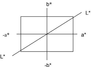
2.4 CIELAB Color Space

yellow-blue axis. These attributes are mathematically defined as nonlinear transformations of XYZ tristimulus space:

L* = 116(Y/ Yn) 1/3 – 16 for Y/ Yn >.008856 (28) L* = 903.3 (Y/ Yn) for Y/ Yn< .008856 (29) a* = 500 [(X/Xn) – (Y/Yn)] (30) b* = .4 x 500[(Y/Yn) – (Z/Zn)] (31)

The three attributes are based on Herring’s color opponent theory with

complimentary colors on the opposite end of the axis. The color space can be shown as:

Figure 5. Plot of CIEL*a*b* space. Where

L*= varies from 0 to 100(L*= 100; prefect diffuser) a*= redness (+) or greenness (-)

-a* a*

b*

-b*

L*

b*= yellowness (+) or blueness (-)

Alternatively, the space can be defined in polar coordinates, known as CIELCH, in which chroma, C*, represents how far from gray an object is when compared to a neutral gray of equal lightness, and hue angle, ho, varies from 0-360. The equation for chroma and and hue is:

C* = (a*2 + b*2)0.5 (32) Hab= tan-1 (b*/a*) (33)

2.5 Single Number Pass/Fail Criteria

For decades, significant effort has been made to develop a single mathematical scale that correlates with visual pass/fail acceptability criteria between two objects, often referred to as a standard and a batch or trial. It was shown that for a Euclidian

color space, the total color difference ∆Εσ between the batch and standard would be the Pythagorean sum of differences between any of the three attributes (Ai = 1, 2,

3)12.

∆Εσ= [Σ (∆Ai) 2]1/2 (34)

I=1 Where ∆Ai = ∆Ai,B- ∆Aii,s.

This approach was not successful when applied to the XYZ system as there was no relation between visual magnitude of color difference and differences in XYZ

2.5.1 CIELAB color difference formula

The simple color difference formula based on CIELAB color space that assumes Euclidean geometry correlates with perceived visual magnitude of color difference is given by:

∆Ε∗ab = [(∆L*) 2 + (∆a*) 2 + (∆b*) 2]1/2 (35) Where

∆L*= L*B - L*S

∆a*= ∆a*B- ∆a*S

∆b*= ∆b*B- ∆bS

and, B = batch and S = standard

In this case, the DE formula produces a tolerance sphere around a given object color, in which pass/fail tolerance is the same in all directions in the space.

2.5.2 The JPC79 color difference formula

In 1979, a color difference formula by McDonald was introduced based on extensive visual data for 600 polyester thread pairs around 55 color centers11.

∆Ε t = [(∆L/Lt) 2 + (∆C/Ct) 2+ (∆H/Ht) 2]1/2 (36) Where

Ht = TCt

T = 1 if C1< .638, otherwise T = .36 + [.4cos (θ1+35]

unless, θ1 is between 164o and 345o when

T = .56 + [.2cos (θ1+168)]

The subscript 1, denotes the standard of a pair of samples.

This formula was used by JP Coats as an internal instrumental pass/fail tolerance, but was later revised by the Colour Measurement Committee (CMC) of the Society of Dyers and Colourists in the U.K.

2.5.3 CMC (l: c) Color Difference Formula

It was discovered that the JPC79 formula produced erroneous data related to the chromatic differences near the neutral axis; that is, the calculated color differences correlated poorly with visual assessments for neutral colors. Also, a discontinuity in lightness differences near the lower values of L* was also observed. Hence, the JPC79 formula was modified to give a new formula, now known as CMC (l: c) 12_, which is now a standard for the American Association of Textile Chemists and Colorists (AATCC), the American Standards and Test Methods (ASTM), and the International Standards Organization (ISO). Hence, it is used throughout at the global textile industry as the primary method of instrumental pass/fail assessment. The formula is defined as follows:

where,

SL = 0.040975 L*ab, 1 / (1+ 0.01765 L*ab, 1) unless

L*ab, 1 < 16 when SL= 0.511

Sc = 0.638 + 0.638 C*ab, 1 / (1+0.0131 C*ab, 1) SH= Sc (Tf + 1-f)

Where f = [C*ab, 14 / (C*ab, 14 +1900)] ½

T = .36 + [.4 cos (hab, 1 + 350)] unless hab, 1 is between 164o and 345o then T = .56 + [.2 cos (hab, 1 + 168o)]

and where

L*ab, 1, C*ab, 14, _{hab, 1 is that standard of the pair samples.}

The scalars, SL, SC, and SH, produce an ellipsoid tolerance, the size and shape of which is dependent on the location of the standard in space. The variables, l and c, can be manipulated to define the ellipsoid for a given application. In textiles, since the dependence of lightness on overall color difference is less than other attributes due to texture properties (unlike, for example, paint chips) the recommended value for l is 2 and for c is 113.

2.5.4 BFD (l: c) Color Difference Equation

Two extensive sets of data, containing both textile and nontextile samples, were used by Luo and Rigg to develop a new formula known as BFD (l:c)14. When visual chromaticity ellipses, obtained from various visual experiments, are plotted in the CIELAB a*b* diagram, they do not point towards the axis in the blue region, and this effect was taken into account in the following formula in and attempt to improve the correlation.

∆ΕBFD = [∆LBFD/l) 2 + (∆C*ab/cDc) 2+ (∆H*ab/DH) 2+

RT (∆C*ab ∆H*ab/DcDH] ½ (38) Where 2 / 1 )] 14000 4 * /( 4 * [ ) 1 ' ( ) * 00365 . 0 1 /( * 035 . 0 521 . 6 . 9 ) 5 . 1 ( 10 log 6 . 54 + = − + = + + = − + = ab C ab C G G GT DC DH ab C ab C DC Y LBFD

Depending on the dataset, the performance of the BFD formula correlates as well or better then the CMC formula. In the 1990s, several new formulae were developed in an attempt to further improve the performance. The most notable formulae were from Nobbs, ∆ ELDS, CIE94, and CIEDE2000. The latter was recently formally adopted by the CIE as a general recommended color difference formula.

2.5.5 CIEDE2000 (kL: kC: kH) Color Difference Formula

introduced by Luo, Cui and Rigg15_{. What differentiates this formula from all others is} that the equation was optimized by incorporating four separate, but generally

considered reliable, color discrimination datasets corresponding to thousands of color difference samples. The equation is an attempt to overcome limitations of previous formulas, and is especially designed to improve the correlation with visual assessment for blues, dark colors and near neutral colors. The equation is specified as follows:

Step 1:

L*, a*, b* and C* are calculated as usual

L* = 116(Y/ Yn) 1/3 – 16 a* = 500 [(X/Xn) – (Y/Yn)] b* = .4 x 500[(Y/Yn) – (Z/Zn)]

Step2: L’, a’, C’ and h” are calculated L’= L*

a’= (1+G) a* where G= .5( 1- C*ab7

/ C*ab

b’= b*

C’= (a’2 _{+ b’}2₎1/2 h’= tan-1(b’/a’)

∆L’ = L’b – L’s

∆C’ = C’b -C’s

∆H’ = 2(C’bC’s) 1/2 _{sin (∆h’/2)}

where ∆h’=h’b –h’s

Step 4. Calculating CIEDE2000:

∆Ε00 = [ (∆L’/KL.SL) 2 + (∆C’/KC.SC) 2 + (∆H’/KH.SH) 2 + RT [(∆C’/KC.SC) (∆H’/KH.SH)2_]1/2

SL Function:

A set of visual experimental data was generated by Chou et al.16 which

accommodated samples with different lightness values. Different lightness equations were tested against the data and it was seen that Nobbs equation performed best against the visual data.

SL=1 + .015(L* - 50)2/ [20 + (L* - 50)] 2 SH Function:

A new SH was developed by Berns17 to fit 5 data-sets:

SH = 1 + 0.015C*T where

RT Function:

As the orientation of ellipsoids points away from the achromatic axis in the blue region, the rotational function, RT, was been developed to correlate for pass/fail performance of blue object colors. The reason for the tilt is not known.

a* Function:

Most of the modern color difference equations assume that the ellipses near the achromatic axis are circle which is not the case and therefore, we get poor fit. Rescaling of a*-axis was done so that the extra stretch would make the chromatic ellipses as circles. The a*-axis was also rescaled in such a way that there was a large effect for neutral colors and almost no effect for high chroma colors. The rescaling of a* has given better fit as compared to previous equations.

2.6 Color Perception Phenomena

2.6.1 Color inconstancy

When an object (e.g. a garment) is removed from under one light source and placed under a different lamp with a different spectral power distribution, the human eye is able to compensate for the lighting differences so that the color would look

approximately the same. Hence, a red object looks red under significantly differing light sources such as incandescent and daylight. This phenomenon is known as color constancy and is achieved through the process of chromatic and lightness adaptation38. The actual mechanism(s) by which the brain is able to adapt to the changes in illumination are not fully understood.

Complete adaptation generally takes up to three minutes. Also, it is known that color constancy does not only depend on the illuminant used but also on the geometry of viewing.

able to adapt to the change in lighting conditions. A new chromatic adaptation transform CMCCAT200031 has been introduced which is an improved and simplified version of CMCCAT9732. A forward and reverse mode was used in CMCCat97 (forward mode is the transformation of the trisitimulus values of a sample under non-daylight illuminant to the corresponding color under non-daylight and vice versa for

reverse mode).The reversibility causes problems in CAT97 which has been removed in CAT2000 which also fits better with the experimental method.

2.6.2 Metamerism

The phenomena of metamerism occurs when two object colors have the same tristimulus values but different spectral stimuli. In these cases, the two objects will match under one condition but not another, e.g., under one light source but not another. For metamerism to occur, the reflectance spectra of the two objects should intersect each other at least at three points. Previous studies suggested that the three intersections were fixed but Wyszecki10 showed that the location of

intersection depends on the method of generating a metamer and it should have at least three intersections. There are four different types of metamerism:

2.6.2.1. lluminant metamerism

The degree of metamerism of two objects that match under a specific light is given as the color difference ∆E between the two objects under a different illuminants, and

MI = ((DL1*2_-DL*22_{)+ (Da1*}2_-Da*22_{)+ (Db1*}2_-Db*22₎₎0.5

Where subscripts 1 and 2 denote illuminant 1 and illuminant 2, respectively.

2.6.2.2. Observer Metamerism

As the color matching functions of two people will vary to differing extents, a pair of metamers may match for one person while it might be a mismatch for another person, all other conditions remaining the same. This is known as observer metamerism. Importantly, even if a color difference formula predicts a match between two objects, it might not be a match to any real observer as the color matching functions of the observer may be significantly different to that of the standard observer.

2.6.2.3. Field Size Metamerism

The angle of viewing and object has an effect on the color perception. A pair that seems a match at a distance might not be match when brought closer.

2.6.2.4. Geometric Metamerism

3 Retail Lighting

A key component of color control in the textile supply chain is the lighting used in the area in which a textile product is displayed to a consumer. While many products are purchased via the internet, or via mail order, most products are purchased from retail stores. Hence, the lighting conditions, such as type of lamp, brightness, color

rendering properties, are critical variables that influence the perception of the colors of garments.

In general, the retail color managers, which provide a critical and growing function in the specification and control of the textile supply chain, do not today become heavily involved in the lighting specifications developed by retail stores. This section

provides an overview of the key factors that lead to variability in retail lighting as well as some recommended 'best practices' from the point of view of lighting engineers [ref].

3.1 Lighting design

3.1.1. Lamp selection

a) For merchandizing areas: most lamps used are fluorescent cool white lamps, deluxe warm white, incandescent and so-called tri-band lamps (e.g., commercial lamps such as Ultralume U3000, U4100 and U5000).

b) For store and mall lobbies: most lamps used in lobbies consist of mercury vapor and mercury halide lamps39.

In general, lamps are selected based on the store design, merchandize, space and economic considerations. Other criteria selecting the lamps involve lumen rating, life expectancy, chromaticity, color rendering, luminous efficacy, maintenance,

ventilation, and even acoustics40. [A number of different categories can be considered for the use of different lamps, as indicated below.

3.1.1 Luminaire

A luminaire19 _{is a lighting system that is an apparatus to enable the control and} electrical distribution of the lamps in a cluster. According to the application and utilization of lamps, the CIE has classified luminaires into six main categories: direct, semi-direct, direct-indirect, diffuse, semi-indirect and indirect. In general lamps by without modification are a source of high glare, but these can be controlled by use of diffusers.

3.1.2 Light diffusing methods

baffles or louvers are used to enhance the diffusion. A baffle is a partition that is placed parallel to the direction of the (usually fluorescent) lamps and between two lamps, whereas a louver is a group of baffles of an egg crate arrangement that are placed below the lamps. Louvers are usually used where low ceiling brightness is required.

Materials that reflect the light into a given direction are also commonly used. Reflectors are of two types: specular and semi-specular which are mounted above the lamps to redirect the upward component of the flux; in general reflectors are used with incandescent and HID sources. For fluorescent lighting, diffuse reflectors are also used.

3.1.3 Lighting variability

Even if a store is designed to provide a specific illuminance level and particular color rendering properties, there are many factors that over time will affect the quality of light that illuminates products. These variables must be adequately controlled to prevent loss of illumination quality. Even redecorating a store with no change in lighting design can affect lighting quality significiantly. For instance, dark walls will absorb more light than pale colored walls. If the reflectance of the wall is increased, the inter-reflected light within the room increases and higher percentage of light will reach the illuminated space. Hence, the surrounding environment will therefore influence the perception of the color of objects, notwithstanding the effects of

general retail stores should be decorated so that wall reflectance should be in the 50% to 70% range, preferably with Munsell values of 7.5 to 8.5

3.1.3.1 Light loss and non-uniformity factors

To maintain average uniform illumination within a store, the initial lumens emitted from the lamp should be higher to compensate for the rapid light loss in the first few hours of burning. However, there is a loss in lumens with the passage of time. Some of the lighting variability is recoverable, whereas others factors lead to nonrecoverable changes.

Recoverable Factors included lamp burn-outs, lamp lumen depreciation, and dirt build-up on surfaces. Lamp burn-outs (LBO) should be replaced, preferably on a regular schedule to prevent excessive loss of illuminance. It is possible to calculate a LBO factor which is the ratio of the remaining lamps lighted to the total number of lamps and develop a protocol to replace lamps when the LBO reaches a

predetermined level.

Dust and dirt accumulation on lamps is a surprising significant factor in reducing the reflectance of luminaires as well as reducing transmittance through lenses. In addition, dirt on general surfaces in the lit area reduces light reflection.

Additional, non-recoverable factorsrelated to lamp brightness depreciation include: pressure and temperature changes in fluorescent lamps, voltage variability,

3.1.4. General considerations for illuminance

Illuminance at a given point can be calculated by the inverse square law20 is given as

E = I / D2 where E= Illumiannce …, I= luminous Internsity

When illuminance is calculated at a point that is not normal to the source, and the area over which the flux is distributed is greater than 1 sq.feet, a correction should be made .For a retail store, the reflection for walls and surfaces can be taken into account4:

E = (lumens per luminaire) (RRC) (LLF) Area per Luminaire

where, RRC = reflected radiation co-efficient, LLF = Light loss factor

area to another. In some cases there will be a sudden loss of ability to see the details of the object. Hence, it is recommended that the ratio of illumination for an illuminated area to the general area lighting should not be more than 5:1 at any place in the store and should not be less than 3:122. In addition, diffuse lighting should be used throughout the store to remove shadows and harshness of direct lighting.

The recommended illumination levels for merchandizing, including showcases, is in the range 750-1000 lx23. For areas not expected to be visited often 300 lx is

sufficient. However, displays should be illuminated between 2000 and 5000 lx.

3.1.5 Factors affecting an observer's visual comfort in a retail store

There are, of course, many factors that affect visual comfort of observers in a store. Some of the more important factors are described below.

Transient adaptation

Viewing angles

The size of merchandise is fixed, but the angle of illumination and viewing can be controlled to maximize visual acuity.

Contrast

Visual comfort depends to a large degree on the contrast between the merchandize and immediate background. Less contrast means significantly more time is required to differentiate the details of a given object.

Glare

Glare24 _{is the excessive brightness in the field of view that causes loss in visual} performance and visibility. It is caused by the reflected light from a surface leading to significant discomfort. One of the forms of reflected glare is called veiling

reflections, which is the reflection of large windows and fluorescent luminaries on the surface being viewed. The effect of lighting variability on visual comfort has been modeled25.

3.5.1.1 Psychological factors

a) observers can be made to feel relaxed using warm (yellow-orange) lights in addition to general fluorescent lighting.

b) light at longer wavelengths such as red increases intensity and anxiety in some people27.

c) lamps with different spectral power effect the perception of strangers28 and therefore comfort level is influenced.

4. Research Proposal

The effective control of color throughout the textile supply chain is of significant importance. Considerable management and control of the color variables is

maintained during the design, manufacturing and approval process through standard lighting and viewing conditions. When the merchandize is placed in the retail stores, the standard conditions are not maintained any more and hence there is a possibility that the color of the merchandize might look different in the retail stores. For this purpose, lighting measurements were carried out in departmental stores and in different stores of the same retailer. There are various factors that can contribute to the visibility and a different perceived color of an object as compared to its

to other stores. The lighting quality in different light booths is also measured to see if there is any significant variability.

A color difference equation is used to test as to how much there is a difference between a trial and a reference pair. The performance of DEcmc and CIEDE2000 was seen using 850 samples under three different lamps and the shift of the same samples in the color space was seen which provides further evidence that since the equations are made based on D65, a form of chromatic adaptation should be

II. EXPERIMENTAL

1. Equipment

Spectroradiometric measurements were made using a calibrated handheld LightSpex spectroradiometer by GretagMacbeth. The spectroradiometer was equipped with a 256 photodiode array and cosine receptor that collected all incident light over a 180 angle. In all cases, two measurements were made at each location and the data averaged.

Ahiba Texomat (1000 control unit) was used for dyeing the metameric

pairs.Spectrophotometric measurements were made using a diffuse integrating sphere geometry spectrophotometer, Datacolor Spectraflash SX. Reflectance measurements were made in the following set up: specular included, UV included, and three measurements were made with 90 rotation of the sample each time, and the data averaged. Colorimetric data were calculated using various standard illuminants (and 'custom illuminants', as described below) and the CIE 10 degree supplemental standard observer.

2. Retail store measurements

A large global retail company was selected for the purpose of this study. The

The lighting in four of the retail company owned stores were measured along with three different departmental stores that carried the company's merchandize. The size of the store ranged from a very small to a very large store with four levels of retail floor space. Two (Store D & B)stores had large entrance/exit areas exposed to external daylight. Two (Store A & c) stores were a part of a mall and the entrance of the store was exposed to indoor lighting of a mall

.

Retail Company's Own Stores Departmental Stores Store D (Expose to Day Light) Store A

Store E Store B (Expose to Day Light) Store F Store C

Store G

2.1 Data evaluation

The irradiance data collected for each measurement in the store was converted to standard ASTM tristimulus weighting functions (table 5 data) for a 100 observer [using a custom program developed by GretagMacbeth48 .Metamerism indices, color inconstancy indices and DEcmc (2:1) was calculated for each custom illuminant for the metameric textile sample pair [which one??] described below. The CIE 1964

Supplemental (100) standard observer was used for the calculations. The Correlated Color Temperature, Lux and Color Rendering Index were directly calculated from the spectroradiometer using the GretagMacbeth LightSoft software. The illuminance values (lx) were calculated for the CIE photometric 100 _observer.

Statistical analysis of key colorimetric data for each store was calculated .The distribution of data was seen to be not normal therefore non-parametric tests44_were applied to analyze it.A non-parametric test is a hypothesis test that does not require any specific conditions about the shape of the population. The Wilcoxon signed rank test is used to see if the two dependent variables were selected from the same population where as in Kruskal-Wallis test three or more variables can be shown if they are from the same population or not.One-way Chi-Sqaure tells us if there is a significant difference between the variables. Other statistical methods such as S.D, upper and lower limit were also calculated.

Spectroradiometric measurement of seven different standard light boxes were taken. All the light booths were in practical use on a regular basis and were intended to be representative of the majority of light boxes used by the textile industry. Three of of the light boxes were fluorescent based daylight simulators, and four were based on filtered tungsten lamps. The light boxes used were:

A = GretagMacBeth SpectraLight III E = GretagMacBeth Judge-II

B = GIT/Datacolor International F = GretagMacBeth SpectraLight III C= GretagMacbeth Spectra Light Jr. G= Unknown

D = GretagMacBeth Judge-II H= Unknown 4. Preparation of Metameric Pairs

Two standard and batch metamers were dyed on 100% cotton twill using reactive dyes, as described below.

Sample Pair A

A 'standard' khaki sample was prepared by dyeing 100% cotton twill fabric using vinylsulofone-based reactive dyes with the standard recommended procedure by the dyestuff manufacturer at 60 oC .A sample size of 10.0 g was used with a liquor ratio of 20:1. The dyes and auxiliaries used for the dyeing were as follows:

Remazol B Blue RSP .0396 g Remazol G ORG F2GS .01192g Remazol Yellow RR .04389 g

Na2CO3 4g/L

Glauber’s salt 35g/L

An identical procedure was used to dye a 'batch' sample, but using a different set of dyes to obtain a metameric match. The dyes and auxiliaries used were:

Remazol Br Yellow 3GL .1896 g Remazol Red RR .0211g Remazol Blue RR .0258 g

Na2CO3 4g/L

NaOH (100%) 2ml/L Glauber’s salt 35g/L

Sample Pair B

A second blue standard and batch pair was prepared was prepared in the same method described for sample pair A above. The recipe for the standard is as follows:

Remazol TURQ GA .9581g Remazol B Red 3BS .1936 g Remazol Orange F2GS Liq 25% .7702g

Na2CO3 4g/L

The recipe for the batch was as follows:

Remazol Br Yellow 4Gl 150% .1190g Remazol Red RR .0151g Remazol Blue RR .2152g

Na2CO3 4g/L

NaOH 2ml/L Glauber’s salt 45g/L

The standard used for sample pair B was found to be significantly color inconstant, and was therefore used to find the variation of color inconstant indices with different custom illuminants.

5. Comparison of the performance of CIEDE2000 and DEcmc via visual

assessment.

following criteria: The samples were to be made into separate high quality garments and were to be hung on a clothing rack and sold together.

AATCC Evaluation Procedure 9 was used for visual assessment with the following set up: 0/450 geometry was maintained using a GretagMacbeth Spectra Light III with a calibrated filtered tungsten daylight simulator. The fabric sample size was about 4” by 6”. In order to obtain enough expert observers, the experiment was executed during three separate color science conferences/symposia over the course of seven months. At each stage, the light source was calibrated prior to use and spectroradiometric measurements taken, using a calibrated GretagMacbeth

Lightspex spectroradiometer, to ascertain that no significant variability was observed in the viewing environment between locations.

Table 1. Colorimetric data of color centers (CIELAB, D65/10o observer) L* a* b* C* hº

LG Std 63.20 -1.43 -0.36 1.48 194.28 MG Std 58.99 -1.65 -0.83 1.85 206.57 Navy Std 25.11 -7.25 -9.37 11.85 232.25

Blue Std 58.00 -5.09 -34.67 35.04 261.65

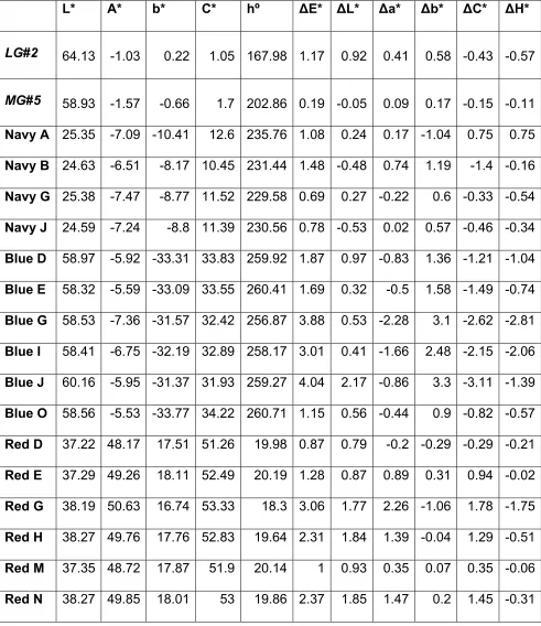
Table 2. Colorimetric data of sample pairs (CIELAB, D65/10o observer).

L* A* b* C* hº ∆E* ∆L* ∆a* ∆b* ∆C* ∆H*

LG#2 _{64.13 -1.03 0.22 1.05 167.98 1.17 0.92 0.41 0.58 -0.43 -0.57}

MG#5 _{58.93 -1.57 -0.66 1.7 202.86 0.19 -0.05 0.09 0.17 -0.15 -0.11}

Navy A 25.35 -7.09 -10.41 12.6 235.76 1.08 0.24 0.17 -1.04 0.75 0.75

Navy B 24.63 -6.51 -8.17 10.45 231.44 1.48 -0.48 0.74 1.19 -1.4 -0.16 Navy G 25.38 -7.47 -8.77 11.52 229.58 0.69 0.27 -0.22 0.6 -0.33 -0.54 Navy J 24.59 -7.24 -8.8 11.39 230.56 0.78 -0.53 0.02 0.57 -0.46 -0.34 Blue D 58.97 -5.92 -33.31 33.83 259.92 1.87 0.97 -0.83 1.36 -1.21 -1.04 Blue E 58.32 -5.59 -33.09 33.55 260.41 1.69 0.32 -0.5 1.58 -1.49 -0.74 Blue G 58.53 -7.36 -31.57 32.42 256.87 3.88 0.53 -2.28 3.1 -2.62 -2.81 Blue I 58.41 -6.75 -32.19 32.89 258.17 3.01 0.41 -1.66 2.48 -2.15 -2.06

Blue J 60.16 -5.95 -31.37 31.93 259.27 4.04 2.17 -0.86 3.3 -3.11 -1.39 Blue O 58.56 -5.53 -33.77 34.22 260.71 1.15 0.56 -0.44 0.9 -0.82 -0.57 Red D 37.22 48.17 17.51 51.26 19.98 0.87 0.79 -0.2 -0.29 -0.29 -0.21 Red E 37.29 49.26 18.11 52.49 20.19 1.28 0.87 0.89 0.31 0.94 -0.02 Red G 38.19 50.63 16.74 53.33 18.3 3.06 1.77 2.26 -1.06 1.78 -1.75 Red H 38.27 49.76 17.76 52.83 19.64 2.31 1.84 1.39 -0.04 1.29 -0.51 Red M 37.35 48.72 17.87 51.9 20.14 1 0.93 0.35 0.07 0.35 -0.06

6. Performance of CIEDE2000 and DEcmc under different illuminants

III. RESULTS AND DISCUSSION

1. Metameric Pairs

Figure 6 shows the reflectance spectrum of the turquoise standard and batch pair. The pair is highly metameric owing to the reflectance curves intersecting at four distinct points. Table 3 shows key colorimetric data for the metamers.

Table 3. Colorimetric data for the standard and the trial metamers.

L* a* b* DEcmc C.I M.I

Standard 57.02 -6.19 -6.92

Trial

D65 57.17 -6.5 -7 0.32 Ref Ref

A-10 55.95 -4.92 -9.84 6.23 3.4 7.17

CWF 55.58 -4.67 -9.26 1.72 3.47 2.33

0 10 20 30 40 50 60 70 36 0 39 0 42 0 45 0 48 0 51 0 54 0 57 0 60 0 63 0 66 0 69 0 Wavelength (nm) % R efl ec tan ce Standard Trial

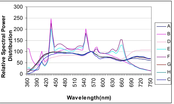
2. Light Booth Measurements

There are two kinds of lamps used to simulate daylight in standard light booths: filtered tungsten (as used solely by GretagMacbeth Spectralite III light boxes) and various fluorescent light sources with varying spectral power distribution (SPD). AATCC Evaluation Procedure 6 [ref] allows for various simulators to be used, although the quality of the simulator is defined based on color rendering index. It is not known, however, how significant the variability in actual daylight simulators will affect practical visual color difference assessment.

Figure 7 shows the variability in the SPD for the daylight simulators used in this study. Clearly the large SPD variability will likely produce significant variability in visual assessment of color difference pairs, particularly metamers. Furthermore, color inconstant samples may also appear to be significantly different colors when viewed under different daylight simulators with different SPD.

0 50 100 150 200 250 300

360 390 420 450 480 510 540 570 600 630 660 690 720 750

Wavelength(nm) R e la ti ve S p ect ra l P o w e r Di s tr ib u ti o

n A_B

D E F G H C

Table 4 shows a summary of colorimetric data for the turquoise metamers when calculated using each of the SPD data for the standard light booths. Clearly the variability in DECMC is high.

Table 4. Summary of colorimetric data for turquoise metamers using SPD data of standard light booths.

DEcmc C.I M.I CCT CRI Lux

A 0.86 1.07 1.06 5428 92 256

B 1.25 0.64 0.95 6802 87 1457

C 0.87 0.2 0.48 6595 96 1612

D 0.87 1.3 1.25 6255 93 1671

E 0.88 1.18 1.32 6695 93 583

F 0.63 0.33 0.3 6559 95 1434

G 0.67 0.27 0.3 6479 96 1470

H 0.89 0.21 0.48 6640 96 1234

I 0.86 0.22 0.45 6617 96 1086

3. Measurement of Stores

The lighting in four of the retail company owned stores were measured along with three different departmental stores that carried the company's merchandize. The size of each store ranged from a small (ca. 2000 sq.ft) to a very large store with four levels of retail floor space. A few stores had significant exposure to external

daylight, while other stores were exposed to indoor lighting of a mall area.

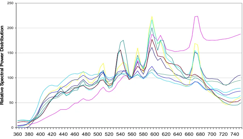
3.1 Store A

the store. Figure 8 shows the variability in spectral power distribution for the xx measurements at various locations. Figure 9 shows calculated DECMC data and indicates the location of each measurement.

0 200 400 600 800 1000 1200 1400 1600 1800 2000

360 380 400 420 440 460 480 500 520 540 560 580 600 620 640 660 680 700 720 740

Wavelength

SPD

Figure 9. DECMC data calculated using SPD data and blue metamers for Store A.

Figure 10. Color inconstancy index for standard blue metamer for store A.

The blue standard is considerably color inconstant under standard illuminants, and although Figure 10 shows a high color inconstancy index value for all locations in the store, the value is relatively consistent, ranging from 3.2 - 5.7. One possibility for further research is to devise an experiment to determine the significance of the color inconstancy index values on visual assessment. To date, this has not been

demonstrated for practical (industrial) color assessment.

viewing experience for a consumer. For instance, the details of very dark samples viewed under low illuminance conditions (e.g., 300lx) will not be easily discerned.

Figure 11. Illuminance values for the various locations of store A.

3.2 Store B

One of the problems that is often experience in stores exists in the over-lapping 'zones' between two different display areas. Store designers produce different experiences by creating different background environments and, often, by using different lamps. This is the case for store B, as indicated in Figures 12 and 13, which shows that at least two different lamps are used in this store.

In such a case, the merchandize placed in the border zone will be affected. In the figure below, we can see that in the men’s section the DEcmc values vary