Fast simulation of queueing networks using stochastic gradient techniques and importance sampling

Fast Simulation of Queueing

Networks Using Stochastic

Gradient Techniques and

Importance Sampling

M. Devetsikiotis

w.

A.

Al-Qaq

J.

A. Freebersyer

J.

K.

Townsend

-Center

for Communications and Signal Processing

Department of Electrical and Computer Engineering

/North Carolina State University

Sublllitted to IEEE/J1CM Transactions on Nciuio rkiruj

Fast Simulation of Queueing Networks

Using Stochastic Gradient Techniques and

Importance Sampling

Michael Devetsi kiotis], }\I/ember, IEEE Wael

A. AI-Qaq,

Student Member, IEE1~ James

A.

Freebersyser, Student Member, I/~EE

J. !(ei Ih Townsend, 1\1ember, IEEE

[Dept. of Systems t~ Computer Engineering

Carleton UJ1iversity

Ottawa, Ontario J(IS GU6, Canada

l"el: (613) 788-2600, Fax: (61:3) 788-5727

Dept. of Electrical & Computer Engineering North Caroli na State Universi ty

Raleigh, North Carolina 27695-7911 , U.S.A.

'"J~cl: (919) .515-G200, Fax: (919) 515-5523

Abstract

To obtain large speed-up factors in Monte Carlo simulation using irnport.ance sampling

(IS), the modification, or bias of the underlying probability measures must be carefully

chosen. In this paper we present two stochastic gradient optirnizat ion techniques that lead to favorable IS parameter settings in the simulation of queueing networks, including queues

with bursty trafIic. Namely, we motivate and describe the Stochastic Gradient Descent

(SCI)) algorithm, aud the Stochastic [lmporimit Event) F1'equcn('y Ascent (SFA) algorithm.

'vVe demonstrate the effectiveness of our algorithms by applying them to the problem

of esl.imal.ing the cell loss probability of several queueing systems: first, a queue with an

Interrupted Beruoulli arrival process, geolnetric service times, and finite capacity 1< (denoted

here by IBP/Geo/1/1<:); then, single and tandem configurations of queues with two arrival streams, a Modified Interrupted Bernoulli stream and a Markov Modulated Bernoulli stream

with batch arrivals, deterministic service times, and finite capacity I( (denoted here by

M-IBP+MlVIBBP/D/l/I\).

Such queueing systems arc useful building blocks in performance

models for ATM nodes and networks. Speed-up factors of 1 to Horders of magnitude over

conventional Monte Carlo simulation are achieved for the examples presented.

1. Manuscript received:

-2. This work was supported in part by the Center for Communications&Signal Processing, North Carolina

State University, and by the Telecommunications Research Institute of Onl.ario, Project on Interconnected

Networks for Multimedia Traffic. James A. Freebersyser is supported by the U.S. Air Force Palace Knight

Program, Wael A. AI-Qa<lis an IBM Graduate Fellow.

3. Portions of this paper were presented at the IEEE Global Telecommunications Conference, GLOBECOM

'93, Houston, November 29 - December 2, 1993. Other portions of this paper have been submitted for

Fast Simulation of Queueing... , Devetsikiotis, AJ-Qa([, Freebersys(:r, and Townsend 1

1

Irit.ro

duct

ion

A significant problem when using Monte Carlo (MC) simulation for the performance analysis of couuuunication networks is the long run times required to obtain accurate estimates.

Under the proper conditions, Importance Sampling (IS) is a l.cclmiquc that call speed lip

simulations involving rare events of network (queuei'lg) systems [1,2,3,4,5].

Large speed-up factors in simulation run time Ca.1I be obtained by using IS if the

modifi-cation or bias of t1)(~ uuderlyiug probability measures is carefully chosen. It is not typically

possible to analytically ruinimize the variance of tho importance sampling estimator, or 18-variance., with respect to the ISbiasing parametersettings for la.rg(~ [multiqneuc] networks

with bursty traffic. Fast simulation methods based on Large Deviation Theory (LDT) [1, 3]

utilize asymptotical a.na.lytical knowledge, and analytical/uumerical manipulations of t.he

system statistics which are not feasible formany realistic systems, An example of the corn-plexity involved with such analysis is the recent extension of Ll.l'I'<type solul.ious to a large

class of mull.iqueuc networks with input traffic consisting of multiple Markov-modulated

Poisson strearns [5J.

A

technique [or Iindiug near-opt.inial

bias

parameter values,

based

OIl repetitive, short

sirnulation r1111S and statistical measures of performance, which included statistical estimates

of the estimator variancehas been previously presented[6]. Such techniques are not restricted

to any specific type of random process, and do not require any knowledge of the internal

workings of tile system being simulated. The Mean-Field Annealing

(MI(A)

global

optimiza-tion algorithm, which is a Iorrn of Simulated Annealing (SA), has also been used forfinding near-optimal

IS

biasing parameter values for queueing system simulation [7]. The MFA

ap-proach is very effective and general, but can be affected

by

long run times and dimensionality

problems,

In [8]

vee Iorrnulated

stochastic

gradient techniques

in the different context

of

digital

communication systems. In this paper we present two stochastic gradient optimization

Fast Simulatioll of (Jueueillg... , Devetsikiotis, Al-Qaq, Freebersyser, and Towusetul :2

Frequency Jlscc11,l (SFA) algorithm involve

Me

estimates of the gradient of a cost function

using likelihood ratio mclliods, as described in [9, 10, 11, 12, 13]. Tile SeD uses estimates of the IS-variance and its gradient with respect to t.he biasing parameters, and follows a

stochastic steepest descent path to near-optimal IS settings. The SFA uses estimates of the

biased [requeiicu oj utuioriani events (I~IE), e.g., cell-loss frequency, and its gradient with respect to the biasing parameters, and searches for thc' minimum IS-variance in the direction of steepest ascent ill the FIE.

vVe illustrate thp effectiveness of tile techniques with numerical e xamples. Large

speed-up factors

(1

to 8 orders of magni tude) over canveil tional

Me

si mulation , at low cell loss

probabilities (e.g., 10-]3) are obtained for queueiug systems with bursty traffic, including

single

IBP

/Geo/

1/1(

queues, and single

and tandem M-IBP+MM BJJl)/D/1/1<.

queues.

2

S'irrrula

t

iorr

of Comrnunicat ion Networks

2.1

M'C Est irnat ion in Network Analysis

Let Xi be the vector or observations relevant to a slot ted-t.ime communications network at time i. Assume that {Xi}i~O is a discrete-time Markov chain wit.h transition matrix P. In

addition, assume that {Xi}i~O has a steady-state distribution, and converges in distribution

to X. Following the formulation in

[14],

the goal is to estimate the expectation E[f(X)] of

some function J(X)

==

h(X)/g(X). Let r be a regeneration state. Then , the expectation of

f

can be written as

(1)

where X o = r, and Tl is the first time greater than zero that Xi == r.

2.2

Efficient Simulation Using IS

To obtain an est.imator of (1), first write

/-/(s)

=

I:r~~1

h(Xi)

and

G(s)

=

I:r~;~l

y(Xi),

where

s denotes a sample path in the evolution of the system under study. Let

Ep[G(s)]

denote

Fast Simulation of Queueing... , Develsikiotis, Al-Qaq, Freebersyser, tuid Townsend 3

observation that the expectation E[G(s)] under measure P can be written as Ep[G(s)] Ep",[G(s)L*(s)J, wlwre L"'(s)

=

P(s)/ P"'(s) and provided that P"'(s)

i=

0 whenever G(s)P(s)

=1= O. L* is a likelihood ratio or, ill the language of IS, a weight Iuuction. Then Elf] can be estimated by

E;:[f]

=

I/N

L~=I L;;~I

h(XidL'ik

I

I

!v!L~~l L;;~I

g(Xik)Lik

where

Lik

=

P(XOk, · .. , X ik)/ P*(XOk,' .. ,Xik).

In general, the uumorator and denominator of (2) can be estimated separately, with M

f:.

N and different IS distributions

[1tI].

Let the transition probabilities of the Markov chain he p(Xj ,Xj+I ) . Within each regeneration cy-cle (RC) k, the individual weights

P(Xik, X i+

1,k)/p"'(X

i

k,

Xi+l,k)

must be distinguished from

the total or cuuiulal.ivc weight

Lik'

at time i. Furthermore, when more than one indepen-dent random event clel.ormi nes the trausi tion (e.g., arrivals, service completions), individual weights are again the product of component weights corresponding to these more

funda-mental random eve-nts. Then, by the Markov chain property, and with initial distribution

uubiased under IS,

i-I i-1

L7k

=

II

p(Xj k ,Xj+1,k)1

II

p*(Xj k , Xj+1,k)

j=O j=O

(3)

In (2) above, the likelihood ratio (or weight) at time i during the simulation depends OIl all

random transitions which previously occurred in the same

Re.

For tandem networks, this time dependence will become slightly more complicated.

An additional motivation to use regeneration techniques is to avoid the deleterious effects

of large system memory on the efficiency of

IS. As

was shown in

[2],

nonregeuerative

IS

brea.ks down as the length of the siruulationapproaches infinity. From all IS standpoint, the

memory of the system is increa.sing within each RC~. For cases where true regenerations are rare, techniques based on approximate regeneration [15], batch means, or A-cycles [5], can

be used to obtain approximately independent trials.

In (2)

it

is implied that IS is implemented in a static way, where the modified or biased measures P* do not depend on the state

Xi

at time

i.

However,

the requirements

of

re-generation can be in conflict

with

static IS [7]. Under certain conditions for

the

simulation

Fast Sunulei.ion of CJuelleing... , Devetsikiotie, AI-Qaq, Fteebersyser, itnd Towueenil 4

regenerative aimulal.ion with efficient IS, IS can be used dynamically within each RC, first

achieving ellicieut esl.irnation of the rare event probability involved, and subsequently driving

the system back to t.he regeneration st.ate [7].

2.3

St at iat icnl Opt

irnizat

ion of

t

he IS Est imat.or

It is well known that the general, nou-parametric, globally optimal IS measure represents

essentially a. tautology, since it requires knowledge of the quantity

E[f·]

to be estimated. Most useful an d practical IS schemes are parametric.

In the parametric ca.se, Iindillg the opti mal IS settings can be posed as a 111

ultidimcu-sional , nonlinear opt.imization problem, where the values of the ]8 parameters Blust be set to opl imize some measure of performance, usually the estimator variance, CTJS(P,

P*).

Assuming an exact, closed-form representation of the IS-variance is not available we

have proposed using statistical measures of performance, which are statistical estimates of

the variability (sca.tter) of the IVIC observations involved, and asyrnptotical estimates of the

estiruator varia.nce,

o-Js(

P,l~*), with respect to

the IS

parameter values

[6, 7].

In [7] we useel mean field annealing (lVIFA), a stochastic global opt.imizal.iou algorithm, to perform

this IIIini rnization.

Although very general, the

Ml''A

approach is potentially slow, especially as the

dirncn-sionality of the search (i.e., the number of IS parameters] increases. Therefore, techniques

that perform a directed search through the parameter space (e.g., usi ng deri vati ve

inforrna-tion] while requiring a smaller number of cost function evaluations can provide attractive

alternatives to stochastic annealing techniques.

3

Stochastic Gradient Techniques

3.1

Me

Estimation of

Gradierits

Performance measures of communicaf.ion systems and networks often take the form of an

expectation

a(O)

that depends on a vector

0

=

(0

1 , ••• ,

Od)

of parameters. Examples of such

Fast SiIIlulatioll of(Jueueillg... , Devei.sikiot.is, /\l-Qaq, Freeoersyser, itnd Townsend ,5

delay, and throughput in networks. When analyzing or designing such a stochastic system,

it is often desirable to calculate not only a(6) but also its gradient \7a(O) with respect to

8. Knowledge of V'a(O) facilitates sensitivity analysis, interpolation techniques, and most importantly design optimization methods, where the vector(Jopt is sought that minimizes (or

maximizes] a( 0) [10, 12].

As iII the case of the original expectation a((J), analytical calculation of V'a(8) is of-ten iul.racl.able. Nuruerical calculation may be Feasible or even advantageous under certain

coudil.ious, but is usually inefficient when numerical evaluation of a(0) is time consuming

[11].

l'lle Monte Carlo estimation of derivatives and gradients of expectations, based on

likeli-hood ratios lias been previously investigated ill [9, IU.11, 12, 13]. Ina rather general setting

this approach introduces a change of rneasure and the corresponding likelihood ratio, and then, by essentially int.erchanging the expectation and derivative operators, expresses the

derivative ill question as the expectation of a new random variable. This expectation can be

then estim atcd using lVlC simulal.iou.

Because of their "semi-analytic" nature, such estimates have obvious advantages over

fini

te di

Ilerence a

pprox iIllations

[11].

A

coIIIparison of likelihood ratio techniques with p~r­

turbaiion a1~alys£s(e.g., [16J) is given in [10]. In [13] likelihood ratio techniques are analyzed ill the context of higb Iy dependable Markovian models, and IS is successfully applied to increasing the efficiency of the gradient estimators when rare events are involved.

Focusing OIl a discrote-t ime Markov chain {Xn}l'~Oand following the notation in [12], an

expectat.iou a(lJ)

==

_E09(lJ,Xo, ...,Xl') can also be written as

where for any instant 1~

, Jt((J,Xo ) l

rr

t - l P((},X_{i , X i}+1 )

Ln(lJ,lJ,Xo, ... ,Xn_{) ==}

_(£)'

_{X). P((J' X X· )} Jlu, 0 t=O

,1,

t+l

(4)

(5)

In the

followiug we willuse

_Ln((},(}')

instead

of

Ln(O,(}',X

o, . ·

.,X

lI ) in order to simplify the

Fast Simulation of Queueing... , Devdsikiotis, AI-Qar}, Freebersyser, and Townsend 6

transition probabilities under 0, Jl(O,XO) is the initial state distribution under 0, and T is

a finiLestopping time. Then, Lhe gradient

\7a(O)

is given by

(6)

or

(7)

where

and

(9)

Most oflen one takes 0'

==

O.

When {Xn}n~O has a regenerative structure, tl}(~ above derivation can also be extended

to tile case where a(O)is described by the ratio formula of regcncrativeanalysis [12], and T

coincides wit.hregouerntion epochs.

Clearly, assuming

a unique local minimum, deterrninisticgradient descent algorithms can

have guaranteed convergence to the minimizing point. It is shown in

[11]

that, assuming a unique mini mum, a stochastic descent algorithrn of the Robbins- Monro type [17, 11],

(10)

that uses fvIC estimates of the derivatives based on eqs. (6)-(9) can also be guaranteed

convergence, for the appropriate selection of step size h(n).

3.2

The SGD Algorit hm

We observe IlOW that

the

variance

of

the IS estimator in (2) is also an expectation

Fast Simulation of Queueing... , Devetsikiotis, Al-Qaq, Freebersyscr, and Townsend 7

minimizes this IS-va.riance. Let Z be equal to the ]S estimate in

(2).

Therefore, by letting

a(O)

=

Ep.{(Z -

Ep. ( Z ))2},

where () is the vector of IS parameters in

(2)

that. determine

P";

we can formulate the choice of [S parameter values as a minimization problem (i.e.,

111in9 a(9)) tllat can be tackled according to (10).

Such an approach to optimiziug the choice of IS settings is a natural complement to our previous statistical opl.imization techniques, where we determine near-optimal IS values by observing est.imal.es of the cost function, namely the IS-varia.nce. Its greatest potential

advantage is that, hy exploitingInure prior knowledge and information about the problem at hand (i.e., derivative inlormal.iou], it can potentially zero-in on the opti mal Ib set.tings faster than global search techniques like the MFA and similar annealing methods. The essential diITerence from annealing techniques is that gradiellL-based techniques are local optimization met hods.

Another factor in overall efficiency is the choice of the appropriate step size h(r~). An

h(

11,) small enough to guarantee almost sure (a.s.) convergence can lead to im practically long

run times, while an h(11,) that is too large can lead to divergence, Clearly, a trial-and-error procedure is required to establish the best trade-orr choice.

For a given point () in the parameter space the random numbers used to estirnate

\la(8)

are drawn using ()'

== (}.

Therefore, during the search the simulation sampling distribution is continuously changing while approaching the optimal IS distribution as (} --t (Jopt. Thus, the algorithm tends to constantly improve the IS-variance until the near-optimal is found.

OUf Stocllastic Gradient Descent (SGD) algorithm is outlined illFig. 1.

3.3

TIle SFA Algorit hm

A necessary condition for speed-up when choosing IS settings is that the raw frequency of important events has to be significantly increased with respect to the original sampling

Fast Simulation of Queueing... , Deveisikiotis, Al-Qaq, Freebersyser, and Townsend 8

n {::

a

/*

Initialize iterat.ion count

*/

80 {:: 83tart

/*

Inil.ialize IS parameter values

*/

/*

Perform gr adient descent on estimated IS-variance

*/

/*

until ern pirical precision Q' is suIlicient

*/

do {

Calculate h{n)

/*

(;et new step size

*/

8n+1 {=On - h(1l)

V

va1t

(9_{n )}

/*

Perforrn descent step

*/

Calculate V'li'r(On+l)using NA RC's

Calculate

P

n+1 using NA

rtc's

[~igure 1: Pseudo-code describing the SGD algorithrn.

suggests biasing ill the "direction of steepest ascent. in

FIE",

since this direction maximizes

the increaseill FI~for the same "total" modification of the parameter values. More precisely:

Le t ()

== ()

0 sue h tII at n0

IS

b ia.s illg is a.p pJied an d tlJen itera tiveJy set

( L1)

where PJE(On) denotes the probability of the important event. as a function of 8, until

PIE((}n) saturates, i.e., attains its maximum value. Then pick (}op Irom the above "search

path" such that the IS-variance is miuimum (or near-miuimum ). Clearly, the same likelihood

ratio estima.tion techniques previously discussed call be applied to yield efficient and accurate estimates of the partial derivatives required.

The effectiveness of this directed search procedure is supported by the fact that the t.rue

(or asyrnptotical) global minimum of the IS variance lies on the trajectory (11) for some

interesting cases, namely the case of detection errors in a linear filter under additive white

Gaussian noise

(AvVGN) [18],

and the case of cell loss probability in a M/M/l/I( queue, as

both theory and empirical results indicate. Enlpirical results also indicate that this is true for the case of detection errors in

mildly

nonlinear lilters under

AWGN

(as those in

[3]).

For

all

lVl/M/l/I(

queue the probability that k customers are in the system is given

by

Fest Sill1ulatiol1 of Queueing... ,

Devetlsil{iotis,

AI-Qaq, Freebetsyser, and Townsend 9

0.9

0.8

0.7

0.6

Jl* 0.5

0.4

0.3

0.2

0.1

0.5 0.6 0.7 0.8 0.9

A*

1.1 1.2 LJ 1.4

Figure 2: Example of steepest ascent trajectory for an M/rvl/1/1< queueing system, with A

=

0.5,Jl

=

1.0

and ( = 10. The opt.irnal IS point is A~pt

=

1.0and Jl~pt

=

0.5.

\vhere Ais the arrival rate and It the service rate. The probability that a custorner will be lost is equal to IJK . Let p

==

AI

It. Under IS

and

Dpi<

uPi< up* _

Dpi< (

>.

* )

Olt* = op*

up! -

iJp* - f.L*2

where the asterisk

(*)

denotes the biased quantities, and

o

pj{ *I( -

(1 -

p*I<+1)

+

(1 -

p* ) (

I(

+

1)

p*I<

up* P {l-p*l<+l)2

+

1 -

p*

K

*1<-1

1 - p*l<+l P

Define the steepest ascent trajectoru,

S,

as the path that starts from the point

(A,

tt)

(the unbiased operating point of the queueing system) and follows the gradient of

pj<,

in the space

Fast Simulation of Queueing... , Devetsikiotis, Al-Qilq, Freebersyser, and Townsend 10

A*I

lli

for 1

=

0, .. · ,lmax - 1, with /\~

=

A,It~

=

u; and tL\ ", ~/l' are suliicienl.ly small.

An example of a stcepest ascent trajectory is shown in Figure 2, for A

=

0.5, Il

=

1.0, and

K = 10. Here, ~/\* = ~/l*

=

0.0:35 and lmax

=

200. For the M/M/l/K queue, the optimal

(and unique asymptol.icaljyeflicieut ) 1S operating point is A" = It //* =,,\ similar to what

opt , r'opt. ,

was shown in [1] for the

rVI/l\1/1/oo

queue. For this example (a.lId every other combination

of Aand J.l we tried] the trajectory S did include the optirnal IS point.

Furthermore, ill support of this search path, we observe that the IS-variance can be writtell as

while the FI E call be written as

where 1IE is the indicator function of an important event, and

1./

*(8) is the cumulative weight

of (2). This indicates that increasing the F'IEshould tend to decrease the IS-variance. More

specifically, at 8

==

(}BF (i.e., at the brute-force M(~ point) V

P1/;;(O)

is parallel to VaJs(8), which means that, for a sufficiently small step size

h'(n),

the first step away Irom the

brute-force

Me

point will necessarily lead to a decrease in the IS-variance. Since this alternative

algorithm picks the IS parameter values with theIIIiniruurn variance over the trajectory

(11),

the IS settings chosen have a guaranteed speed-up over the conventional

Me

estimator.

It is reasonable to assume that the

~

PIE estimator will be more accurate [or the same

sample size than the

\la7s

estimator

(~(T;s

involves estimates of second order moments).

Fast Simulation of Queueing... , Devet.sikioiis, AJ-Qil,q, Freebersyser, and Townsend 11

to the biasing parameter values. Also, there are no convergence effects to slow SFA down,

since the gradients guiding the search are not the gradients of the cost function. For these

reasons, following trajectory (11) is rather general and robust, l'l'gardless of the existence of

local minima. in the IS-variance space. Finally, searching along trajectory (11) is guaranteed

to provide speed-up (potentially equivalent to that provided by t.he SGD algorithm).

Partials

0JJ/;;

can be found by replacing a(O)wil.h PIE in eq. (7), where_{g(O,Xo, ... ,X}

_T)

is the number of blocked cells in a RC. Hence

g(0,

X_{o, ... ,}X_{T )}

=

L;~o

h( 0, X_j), where

ue,

X.)

==

{I

if a cell is blocked during slot j J 0 ot.herwise

Choosing the same initial distributions

/1(O,X

o)

=

/1(O',X

o) and

0'

=

0,

and choosing

T,

the end of aRC, as the stopping time, it follows that ~ = 2:J~o ~~ =

2:}=oO

= 0, and

( 12)

Finally, illorder to estimatethe partials of PI

E(

8) with respect Lothe elementsof (J,one can draw numbers using 0, and then take a sample mean over i.i.d. random repetitions of the

quantity in brackets on the right-hand-side of eq. (12). These partial derivatives can then

be used

in the SF'!\.

algorithm.

When irn por tu.nt events are rare the accuracy of \7PIE(8_{n )} will be very poor as long as

PIE is low.

III

[l:J],

IS is applied to \7

PIE((}n)

as follows: Let

a((}n)

== p/E(On).

Then

(13)

where Oil is chosen inorder to increase the accuracy of the estimation. Therefore, we call use

(J" for the sampling distribution to estimate \7PJI'J,(8n ) until [J1E becomes large enough to

a.llow us to start using

On

itself. We call this additional biasing "second-order IS". Heuristic

arguments similar to those we present later forchoosing a starting point for the

SGD

algo-rithm call

be

used for the selection of a favorable "second-order-IS" for the

SFi\.

algorithm.

OUf

Stochastic

(Irnportant

Event)

Frequency Ascent

(SfA) algorithm

is given in

Fig.

3.

Fast Simulation of Queueing... , Devetsikiotis, AI-Q:tq, Freebersyi-er, and Townsend 12

n¢:O

IT-

Initialize iteration COUIlt.

*/

80 ¢:: fJBF

1*

Initialize IS parameter values

*/

1*

Perform gra~ientascent on estirnated "raw'

*/

1*

probabilit.y [)}E(8n ) until saturation occurs

*/

do {

Calculate h(11)

1*

Get new step size

*/

en

+1 ¢= On

+

h(n)~PiE(On)

/*

Perform ascent step

*/

Calculate w(On+I) using NB RC's

Calculate P/E(8n+l ) using NB RC's

} while { PIE(Bn+1 ) - ?IE(8n ) >£ }

Rcturn H, Rn such that v;lr(8n ) isminimum

Figure 3: Pseudo-code describing the SFJ\ algorithm.

....

<f>(1) ... _~(2)

....

pIP""" ... ...

•

•

•

~(S)

Figure 4: General tandem queueing network.

resolution and statistical accuracy. In [6J vve have describeda detailed algorithmic procedure for near-rninirnizat.ion the IS-variance based on statistical estimates taken on an optimal search direction, when simulating digital communication links with linear receivers. In the caseof[6J the optimal direction was the direction of theimpulseresponse of the linearreceiver

filter. The SFA approach essentially generalizes that algorithm by providing a. (heuristic)

favorable search direction for a much larger class or systems.

4

St.och

ast

ic Gradients for Tandem Networks

4.1

Like liho od Ratio Techniques for Tandem Networks

As shown in Figure4, a general tandemqueueing network consists of several stages of queues,

the output of one queue feeding the input of the next queue. Assuming a discrete-time or slotted approach, at least one time slot is need for a cell or packet to propagate through a

Fast Simulation or

Queueing... ,

Devel,sikiotis, Al-Q...

q, Fteeiiersyser,

and

Townsend

13

Let

V~s)

be thc vector of observations representing the state of the arrival processes and

tile queue for stage s of

S

in the t audern network at time i. Let. the vector of observations relevant to

the

tandem network atstage

S

at timei be X·

=

(V~l). V~2) V~S)) '1'he

t 1-.s+1' 1-5+2"'" 1 •

tirne shift in the observations at each stage resul ts Irorn a cell requiring at least aile time slot

to propagate Lh rough each sta.ge. Now {Xi}i~O is Markovian under general conditions. Let

OJs) he the paraun-tcr associated with the [-th random process at stage s for l = 1, ... ,1Tt_s,

and </J(s)

=

(8~s), ()~

s ), ••• ,

O~l,)

be the vector of parameters belonging to stage s so that 0(5)

=

(</J(1) ,</J(2), ... , </J(S)) is t he overall vector of parameters.

All

expectation a(S)(8(S))

=

EO(s)g(O(S),XO, ... ,X_{T )} at the S-th stage in the tandem

network can also IJe \vritten a.s

(5)(0(S)) - E (()(S)

X

X

)/(S)(()(S) (}'(S)

X

X )

a - (}'(S)9 ,0, ... , T JT ., ,0., ... , T ( L4)

where

T

is a finit(, stoppi ng time, The expectation a(5)(0(5)) is ta.ken at the S'-th stage ill

the network, otherwise

5

stages would not be needed in the simulat.ion. We assume that the

optimization of tlte bias parameters is performed Ior only a single expectation which is at

the

S1-th

stage in f.he network, since simultaneousoptimizatiou of multipleestimators could lead to conflicting bias parameter settings that would not result in performance speed-up.

At sta.ge

5

in the tandem network, the likelihood ratio at time 11- during the simulation,

L~S)((}(S)., (}/(S) ,_{X o, ...},X_{n ) ,} depends on all random transitions w hich previously occurred at

stage S' up to time ii, as well as all random transit.ions which previously occurred at stages

1 to S' - 1 at times 11, -

S

to 1~ - 1, respectively. As stated before, this time shift results

because one time slot is needeJ for a cell to propagate through a single stage in the network

due to the slotted time operation of the tandem queueing network, as well as the simulation.

The stages at, positions downstream Irom Sin the tandem network will have no effect on the

Ii k

eli

It

00d rati0 L~:S~)((J(S) ,0/(S) ,X_{o, . . . ,}Xn ) at s t ag<~ S b ecaIIse c(' 1Is

fI

0w 0

III

YfroIIIstage s to

stage s

+

1 in the tandem network. The random processes parameterized by the vector </J(s) are iudependent [rom stage to stage, even though the expectation a(S)(O(S)) is dependent on

Fast Simulation of Queueing.." Deveisikiotis.

AI-Qa.q,

Freebersyser, and Townsend 14

n ¢=

a

/*

Initialize it.eration count

*/

(}(S) n(S)

r

I ' . I'

o ¢=V"tart nitia IZC ISparamel.er values

*/

r

Perform gradient descent on estimated IS-variance

*/

/*

until empirical precision 0' issufficient

*/

do {

C al cul ate It(n) /

*

(~etile w s t e psi ze

*/

n(S) n(S) I ( ... (S) (5')

v n+1 {::: un - t 71.)V'Val" ((Jn' ) /* Perforrn descent step

*/

CaIculate

var(

S) (

e

~;~1)lJsin g NA ftC's

Calculate PS,n+l using NARC's

} w1 ' )11e {J-(S)(uar

e

u+1(S)) /-, PS,n+l"" >n }

Figure 5: Pseudo-code describing the SGD algorithm for tandem networks,

11 at the S-th stage in the network is

n-l P((J(S)

X X

)

L(S)((}(S) (}/(S) X X ) -

IT

,i,

i+l

n ,

,0,,··,

11. - . P(()'(S) X. X. )

%=0 , t , t+l

(15)

where P(0(5),Xi, Xi+1 ) is the transition probabi lit ios under (}(S). In the following discussion,

vee use L~tS)(O{S), (J/{S)) instead of the expression shown ill (15) ill order to simplify the

notation.

4.2

Tile SGD Algorit hm for Tandem Networks

The

SCI)

algoritlun [or tandem queues is outlined in Fig. 5. IS is applied by replacing the

original parameter O~S) with ()(S). 1'lte performance measure of interest is the mean-square

value EO(Sl(PJ)and its gradient with respect to the biased parameters, \lO(slEO(s)(P'§), at

the 5-th stage of the tandem network, where

P

_{s =}

'[)";01

Iy) Lf')(

O~S),0(5)) is the estimate

of the cell loss at the 5-th stage of the tandem network,

Iy)

is the indicator function of a

cell block ill slot j at stage S, and

TheIl,

j - l p((J(5)

X X

)

L(5)(0(5) (}(S))

==

IT

0 , i, i+l

J 0 ' _{i=O P}(_(J(5)_,X· X. )

t, t+ I

Fast Si.lllulatioll of Queueing... , Devetsikiotis, AI-Qaq, Fteebersyser, etu! Townsend 15

~E

1(5)

[(~

/ (5)L(S) ((J(S) (J(S))) 2

L(~)((J(S)

(J/(S))]

DO~S)

(J

Z:: J J 0 ' 1 ,

I )=0

E

_o

[(~

/(5 )L(5)((J(S) (J(S))) 2 aL!.;) (0(5) (}'(S))

I(S) Z:: J J 0 ' ( 9 ) '

j=O

GO

i

-1-

{_a_

(~

/(5)l(5)(O(S) (J(s)))2} L(S)((J(S)

(}/(S))]

(17)

80(s)1 J=O

c:

J..J) 0 ' T ,

where 6 '(5 )parameterizes the actual sampling distribution for tIle S-th stage of the tandem

network. Since

~1J(~) 1'-1

8

[J((J(S)

X· X·

)

L(~)(8(S) (}/(S))

_u_..J1_ ( (J( S ) (J/(S))

==

_~

, ),

)+1 1 ,

( 9 ) '

c:

a

(9) P((J(S) X·

x· )

U()i j=O 0i '~)' J+1

this results in

(18)

1J ·

_51ng L(8)_j (()(S)_{0 '}()(S)) -_- 1/L(5)₎ ((J(S)_,()(S))_{0 ,} to show 1hat

I

Fast lSil11ula.tiol1

of QlIeueing... , !)evc(,sikiotis,

AJ-eda.q,

Freebersyser, sru! Townsend 16

I

t

ki

(}'(S) - (}(5) (. I . . (5)

anc a 109 - i.e., urawuig random numbers uSIng (J ) which implies

L~S)((}(S) ,(J'(S))

==

1, rcsul l.s in

[(

1'_1

. ) 2

T-I

a

(5)

==

E (5) "

I~S)L(S)(()(S)

()(S))

~

P(O ,Xj,Xj₊l ) 1

(} ~)) 0 ' LJ ~) (s) !J((}(S)

)=0 )=0 UBi ,

X

j ,

X

j

+

1 )

(

1' - 1 ) T-I )-1 ~J-J(()(5) X X ) L(5)((}(5) (5) ]

_ 2 , , / ( S )L(S)(O(S) (}(S)) " " I(S)"" U , k , HI J 0 '

e )

~) ) 0 ' LJ J LJ (s) (5)

)=0 j=O k=O aO_i P( ()

.Xs, X

k

+

1 )

(22)

Thus, in order to estimate the partials of the IS rncau-squarc term with respect to the elements of (}(S), numbers should be draw using (J(S), and then a sample mean taken over

i.i.d. random repetitions of the quantity in brackets on the right-hand-side of (22). These

partial derivatives call then be used in the SeD algorithm.

The task ofobt.aiuiug partial derivatives of P(()(S),

X

k ,Xk+l ) is facilitated, among others,

by the multi plicat.ive nature of the one-step transit.ion probabilities (due to independenceof

Lhe raudom choices involved]. For the random processes considered. here, a transition in a

slot depends on all independent (discrete) randall) events, each occurring with conditional

probability IJls) under the origjnal, unbiased. settings. Under IS, these probabilities can be

biased so that Llu-y hecorne O~s)]J~s). Then e(S) = (O~I),...,O~~n and p(e(S),Xi,Xi+d =

TI

s

TInL ...

0t(S)])t(s). leading to s=1 t=1 I

(23)

(24)

1 fJP(O(S),Xi, Xi

+

1 ) _ _1_

P((}(S) X· X.) DO(s) - ()(s)

, I'"'" z+l I l

Several heuristic arguments can be used to identify a start.ing point for the search in

and

(10) when imporf.ant events are rare. For example, near-optimal IS set.tings for a single or

tandem queue case where the important eventsarc not rare (e.g., smaller buffer size for cell

Fast S'iulu/atioll of Queueing... , J]evct.sikiotis, AJ-CJ;t(], Freebetsyner, eiu! Townsend 16

and taking 0/(5)

=

0(5) (i.e., drawing random numbers using 0(5)) which implies

L~)((}(S),(}/(S))=: 1,results in

[ (

,,.- 1 ) 2T-I

~

(5)

=

E (5)

L

!(S)L(S)(O~S),O(S))

~

uP(O ,Xj,Xj+d 1

(} ._ J J

c:

D()~s) /)(8(5) X· X. )

J-O J=O l , J' J+l

(

1' - 1 ., ) T-l j-I ~p(()(5)

X

)

L(5)(()(5) (5) ]

-2

~ l~'~)L(S)((J(S)

(J(S))

~ I(S)~

u ,k,Xk+l j 0 ,0 )

~ J ) 0 ' ~ J ~ (s) (5)

)=0 j=O k=O OOi P(8,Xk,X k+1 )

(22)

Thus, in order to estimate the partials of the IS rncau-square term with respect to tile elements of (}(S), numbers should be draw using 8(5), and then a sample mean taken over

i.i.el.

random repetitions of the quantity in brackets

on

the right-hand-side

of

(22). These

partial derivatives call then be used in the SGD algorif.lim.

Thetask ofobf.ainiug partial derivativesof P(8(8),Xk ,Xk+l ) isfacilitated,among others,

by the multiplicative nature ofthe one-step transition probabilities (due to independence of

the random choices involved}. For the random processes considered here, a transition in a

slot depends on all independent (discrete) random events, each occurring with conditional

probability l)~s) under the original, unbiased settiugs. Under IS, these probabilities can be biased so that they become Ors)]J~s). Then O(S)

=

(O~l),... ,O!,~l) and P(O(S),Xi, Xi+d

=

TI

s

TInt ..

01(s)]JI(s),leading to

s=l 1=1

(23)

(24)

and

1 fJP(O(S),Xi, Xi+1 ) _ _1_

P(O(S),Xi,Xi+d

a()~s)

- ofs)

Several heuristic arguments can be used to identify a starting point for the search in

(10)

when import.ant events are rare. For example, near-optimal IS settings for a single or

tandem queue case where the important events arc not rare (e.g., smaller buffer size for cell

Fast Simulation of Qlleueing... , Devetsikiotis, AI-Qaq, Freebersyser, and Townsend 17

rare event case. "vVewillalso demonstrate that the ncar-optimal bias parameters fur as-stage

tandem queue nel.work can be used as a starting point to quickly obtain the ncar-optimal bias parameters for a

(S

+

1)-stage tandem queue network.

5

Experinl.ental EXalUples

5.1

TIle IBP /Geo/l/K Queue

The IBP/Geo/l/I( queue 1 is the slotted-time counterpart of tile

IPP/l\JI/l/I(

queue 2. For

this queue, although the service process is memoryless, the arrival process is bursty, making

this system a useful aud widely used model for the bursty processes involved in

13-ISDN

and

ATIVI

analyses. Exact solutions for this queue can l,e obtained hy nurnerical solution of the

corresponding Markov chain. vVc include it in our experiments to provide further validation of our techniques, as was also Jane in [7].

There a.re L\VO stales of the arrival process: active and idle.

III

the active state, an arrival

carl occur with probaliility Q while ill the idle state no arrivals can occur. While the arrival

process is in the active sta.te, there is a probability p at each slot that tile state will remain active and a probahility 1 - ]J that it will change to idle. While the arrival process is in the

idle state, there is a probability 'l at each slot that the state will remain idle and a probability 1 - q that it will change to active. When the server is busy, there is a probability 1 - a

ill each slot that a customer will depa.rt. Arrivals and service completions are independent. There is a finite capacity of 1< customers in the system.

In

our experiments, Q was assumed

to be equal to 1. The squared coefficient of variation

C

2 _{of the interarrival times is used to}

measure the burstiness of the arrival process. Typical values are

C

2

₌

1 corresponding to Poisson arrivals,

C

12 _{~ 20 for voice and C}2 _{ranging [rom 10 to 10,000 for video. A numerical}

technique that evaluates cell loss probabilities for this queueing system call be found in [19].

Under regenerative IS, we choose the times that a customer arri ves to all empty system and tIle arrival process has just changed to active, as the regeneration points. In each

Fast Suuuletion

of

Queueing·... , Deveisikioiis, AJ-Qa.q, Fteebersyser, etu] Townsend

18

~

»:

/

/

,

J

r

I

I

I

I

..

--Qj U 1 0.1 0.01 0.001 0.0001 1e-05 1e-06 1e-07 1e-08 le-09 le-l0 1e-ll le-12

10 100 1000 10000

II

Numerical resul ts

IS simulation

Figu re fi: Estimated cell loss probabilities and numerically calculated probabilities [19] for the

II3 P/(]eo/1/ I( queue.

c

2 _{CPU 1'irne, seconds}

10.0 0.731;'

20.0 1.417

30.0 2.099

Table 1: CPU 'I'irne for 1,000 RC's of the IBP/Geo/l/I( queue on a DECStation 5000/25 when no IS is applied (K=200).

regeneration cycle (RC), we bias initially p, qand a to p;, q; and (J"~, until one customer has been blocked, then change IS parameters to

]J;,

q~ and O"~ in order to allow fast regeneration.

III

our experiments, we set

p;

=

]1,

q;

=

q,

(J";

=

(J",

and optimized with respect to the

settings of 0₁ = pUp, O₂

=

q~/q and 03

=

(J"~/(J" using the SGO and the SFA algorithms

from above. Results were obtained for queue set-lips that corresponded to three different

values of

C

2 , namely 10.0, 20.0, and 30.0 (see Table 2). Estimated loss probabilities are in a.greement with the numerically calculated probabilities ill [19), a.s illustrated in Figure 6.

The simulation time required for 1,000 RC's on a OECStatioll 5000/25 when no IS was applied for these three cases is given in Table 1. The queue capacity K was set equal to 200.

In applying the SGD algorithm we used in each case the near-optimal biasing for K

=

50

Fest Simulatioll of Queueing... , Devetsil{iotis, AJ-eJaq, Fteebersyser, and Townsend 19

System Pr[loss] gnpl,Oop2,OopJ Pr[loss] 95%Interval Rn e t

IBP /Geo/I/1< 1.0457 (7.405X10-TI_,

C2

=

10.0,a

=

0.35147,I(

=

200 7.530X 10-12

0.9244 7.536X10-12 _7.666X10-12_{) 1.3X10}8

P

=

0.932075471,q

=

0.954716981 1.0763

IBP/Gco/1/1< 1.0231 (8.1:35 X 10-1

,

C2

=

_20.0,a

=

_{0.35147,I(=200 8.301 X 10-}7 _{0.9586 8.259x 10-}7 _{8.382X 10-}7_{) 1.4X 10}3 P

=

0.9650'18543,q

=

0.97ll699029 1.0'114

I

lBP /Geo/1/1< 1.0156 (4.730X 10-5,

C·2 _{=30.0,a = 0.35147,J(}

=

_{200 ·1.829X 10-}5 _{0.9710 4.809x10-}r

.) 4.887X 10-5_{) 2.1 X 10} p

=

0.976470588,q

=

0.98,1313725 1.0231

Table 2: Est.iruatcd cell loss probabilit.ics and speed-lip factors usuig l.he SGD algor ithrn for the IBP/C;eo/l/I( queue. For these estiinatcs: Nn= 100, Nne = 300.

the corresponding loss probabilities were high and the space could be searched efficiently with the SeD algorif.hm starting Irom the brute-force

Me

point. Furthermore, we used NA == 300 RC's per simulation run for C2

₌₌

_{20 and C}2

₌₌

_{30, and}

IVA

==

3,000 for C2

==

10,

TIle

algoritlun converged in all cases after

ls

<

1,000 iterations. The step size h was

obtained by trial-and-error and varied from 5 x 10-3

(C

2

₌₌

₃₀₎

La 1013

(C

2

==

10).

III

applying the SFA algorithm we used in each case the nea.r-optimal biasing for K

==

50

as the "second-order' IS. Obtaining the near-optimal If biasing for I(

==

.50 was not difficult, since the corresponding loss probabilities were high and the space could be searched efficiently with the SFi\ algoritlun without any "second-order" IS. Furthcrnlore, we used NB = 300 RC's per simulat.ion run for

C

2

=

_{:30, and N}

B

=

3, 000 for C'2

=

10 and

C

2

=

20, The

algorithm required between I

_a

= 300 and I

_a

= 800 to "scan" Lhc search space. The step size li

==

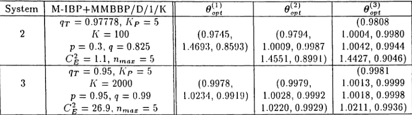
10-4 _{was obtained by trial-and-error. The saturation tolerance Ewas set to 0.05.}

Tables 2 and :~ summarize tile results, incluuiug the near-opt.imal IS biasing parameter

values (Oopl, (}op2, Oop3) found by the

SeD

and the

SFi\

algorithms, respectively, the corre-sponding estimated loss probabilities, the estimated confidence intervals and the speed-up factors with respect to conventional MC simulation. Numerically evaluated loss probabilities were taken Irom

[19].

In order to determine confidence intervals and speed-up factors,

Nn

of

NRC RC's each were run using the chosen IS biasing values. As in

[7],

speed-up factors were obtained assuming consecutive cell losses are independent within each RC for conventional

Fast 11i,nlllaf,;oll

or

Queueing·... , [Jcvcl,si/(;of,is, J\/-Qaq, Frccbcvsvscr, tuu] Townsend 20

Syst em Pr[loss] Oopl , Oop2, OopJ Pr[loss] 95%Interval Rn e t

IBP /Geo/1/1< 1.0444 (S.123x 10-1:l,

C2

=

_10.0,a

=

_{0.35147,}(= 200 7.530X10-}12 _{0.9793 8.136X10-}12 _1.114X10-1 1_{) 4.4X10}5 P

=

0.932075471,q

=

0.954716981 1.0026

IBP /Geo/ l/I( 1.024,1 ( 7 .2,13X10-7 ,

C2

=

_20.0,a

=

_0.35147,K

=

_{200 8.301 X10-}7 _{0.9883 7.807x 10-}7 _{8.372 X 10-}7_{) 8.3}

X10

p

=

0.965048543,q

=

0.976699029 1.0008

IBP /Geo/1/1< 1.0179 (4.S:10 X lO-b,

C2

=

30.0,( j

=

0.35147,K

=

200 4.829X10-'s 0.9925 5.082X

10-r

) 5.633X 10-5_{) Me·} p

=

0.976'170588,q

=

0.98·1313725 1.0001

Table 3: Estimated cell loss probabilities and speed-lip factors using the SFA algorithm for the

IBP/C~~o/l/I(queue. For these estimates: NR

=

100, Nile

=

300. The asterisk (*) is used to denote points where the use of IS did not result in speed-up over lYICsimulation,hence the point used is that found by 1\1 C simulation.

when important events are bursty more such events would have to be observed for the same

statistical accuracy (see [20]). The net run time speed-up over conventional

rvIC

simulation

is denoted

by

R_{n e t} and takes into account the increase in the length of RC's when IS is used.

The speed-up factors given here describe the factor by which an

IS

estimator that uses

our chosen par a.tucter values is more accurate than a conventional lVlC estimator based on

the same sarnple size. TIle computer run time required to search Ior these favorable

IS

values

has not been included in this calculation. For the examples shown here, that overhead would

reduce the overall speed-up factor

by

up to 2 orders of magnitude for some cases.

As expected, the estimated speed-up factors are low for high loss probabilities but increase

consistently as the loss probability decreases. This is a desirable effect since increasing speed-up factors are crucial in order to estimate very low probabilities within a realistic amount of run time. Taking into account this trend, as well as the overhead involved ill the search

for near-optimal IS settings, one can determine in each case the break-even loss probability,

below which employing IS is favorable in terms of total run time required. Our results clearly

indicate that, for realistically low loss probabilities

(~

10-

7) , tile statistically optimized

IS

settings yield significant speed-up factors over Me simulation. Furthermore, near-optimal

Fast Siinuleiion of Queuel·]lg_{-' . . .. ,}

D

_{evelJSI {IO JIS,}1·/·

t·

Ai_-

Q'

_{ltc], rree}D /_{Jel'syser, tuid Townsend 21}

M-IBP

.

.

.

o

q Tagged

~

K1 0 Tagged

T Traffic _Traffic K2

~ ~

p"q, External_Traffic ( External (

I P2'q2 TraHic I

1 -p,

p, q,

1 -q, MMBBP (IBP)

Figure 7: lVl-II3P+l\IMBBP/0/

l/J<

tandem queues.

5.2

M-IBP+MMBBP/D/l/K Tandem Queues

5.2.1 Descript ion

As described in

[21]

and shown in Figure

7,

a single stage of this slotted-time queueing 1110del has one server with a deterministic service rate of one cell per slot. There are two independent traffic streams entering the first stage of the tandem

M-IBP+lVllVIBBP/D/l/I<

queue. The first stream, called the tagged traffic

[21],

is modeled by a Modified Interrupted Bernoulli Process (M-IBP), which differs from the standard

IBP

in that the busy periods have a deterministic, constant length equal to lip slots, where !([> is referred to as the packet size or number of cells in a packet, and one cell is assumed to arrive in each busy slot. When the tagged traffic is idle, there are no arrivals, and there is a probability qr that the traffic

remains idle.

The seconel stream, called the external traffic

[21],

is modeled by a Markov Modulated Bernoulli Process with Batch arrivals (MlVIBBP). It differs Irom the standard MMBP (of which the IBP is a, special case) in that more than one cell call arri ve during a busy slot, i.e.

Fa.st S'ill1ulat;ol1

or

Qlleueing·... , !)cvef,sikioiis,

Al-Qaq,

Freebersyscr, tuu! Towuscus! 22

bi(111, )[or each state i

==

1, ... ,_{N s of} the NllVIBP. Assume the MIvIBBP has two states, active

ancl idle, i.e. an lnterrupted Bernoulli Batch Process

(IBBP).

When the external traffic is

active, arrivals occur and there is a probability ]Jthat the external traffic remains active.

In

state 1, the active state, bI(0)

==

0and arrivals occur with a uniform batch-size distribution,

i.e., b1(rn.)

==

1/1tn t a x for 171,

==

1, ... ,1tm a x ' When the external traffic is idle, there are no

arrivals, and there is a probahilil.y 'l that the external traffic remains idle. In state 2, the

iclle sl.atc, b2(O)

==

1,and b2( 11 1.) == 0 for 17t

==

1, ... ,1t_{11t a x .} When tagged and external arrivals

occur in the same slot, the queue is filled randomly with tagged and external arrivals.

for tandem

configurations of

lV'I-Il3P+lVIIVIBBP

/D/l/I<

queues, p and q are indexed for

each stage as Ps and (Is [or s == 1, ...,.S. Similarly, each queue ill the tandem network has a

finite buffer of length !\"s' The tagged traffic always continues Irom one node in the network

to the next node ill the network, while the external traffic exits the system. Thus, the input

streams of thestages following the

first

stage of the tandem network are characterized by the

taggeu traffic stream exiting the previous stage and an additional MlVIB8P process modeling the ex ternal tramc.

v\l'e denote

by

Cb

the squared coefficient of variation or burst.incss parameter of the external traffic, which describes the variability of the interarrival time of the external cells entering the network at each stage. The corresponding burstiuess parameter for the tagged

traffic interarrival time variability,

C;,

is measured at the input of each stage sill thenetwork

for s

==

1, ... ,S'.

1'he recent attention paid to A'I'M technology has madesj mulatiou of tandem networks of

great interest. Tandem networks of

lVI-IBP+MMBI3P

/l/D/I<

queues can comprise an

end-to-end model of the nodes in an ATM network, where the

M-IllP

lagged traffic represents

tile stream under observation (e.g., a specific virtual circuit), and the

MMBBP

external

traffic represents the aggregation of all the other virtual circuits through the same node.

The deterministic server models the link carrying the traffic to the next node in the network.

A numerical technique that evaluates cell loss probabilities for a single stage of the

M-IBP+MMBBP /D/1/K queueing system is

given

in [21], although the numerical stability

Fast

Sutuiletion

of Queueing... , Deveisikiotis, A/-Qaf], Freebetsyser, tuul Townsend 23

System C~PU 'rilne,seconds

1 O.57:J

2 0.3'1~

3 20.772

TabIe4: CPU TimCfor 1,000 RC'S 0ftile sillgIp tvl-113 P

+

tvl IVt IJB

r /

0 / 1/I( quelJe 0Ita 0 ECStation 5000/25

when no IS is applied.

solution of Markov chains with dimensionality proportional to the queueing capacity, the

requirecl run time quickly becomes forbiddingly long for large buffer sizes and/or tandem

networks of queues. Furthermore, problems with numerical precision and stability may

arrse.

III the following, vve first consider single

M-IBIJ+lY1MBBP /D/l/I<

queues, and then

1\11-IBP+NIlVIBBP /D/l/I<

queues

in

tandem.

5.2.2

St.o chast ic Gradient.s for the Single

M-IBP+MMBBP /D /l/K

Queue

vVe let regeneration epochs be the instants where the queue is empty, the ta.gged traffic

stream is idle, anel the external traffic stream is just going active and isgenerating a cell. In

each

IlC,

we

bias

initially p, q and qr to ]Ji, q~ and qT,t' until

aile

customer is blocked, then

change

IS

pararneters to ]J;,

q;

and QT,2 in order to allow fast regeneration.

In

our experiments, we set I);

==

]J., q; == q, ql\2

==

qr, and opl.itnized with respect to the

settings of 0₁ =

pi!p,

O₂ = q;!q and 03

=

'lr,t/qT using the SeD and the

SFA

algorithms.

For our example cases, the total offered traffic load was held fixed at 0.7, with the offered

external traffic load ranging froIII 0..5 to 0.6. Table 5 describes the system set.-up for our

three example cases (referred to as systems 1, 2, and :3, respectively). The simulation time required for 1,000 RC's on a DECStation 5000/25 when no IS was applied for these three

cases is given in Table 4.

In applying the SeD algorithm we used the same approach as in the previous subsec-tion, always starting with a small queue capacity and increasing until we reached the desired capacity. In each case we used the near-optimal biasing for the immediately smaller queue

Fast

Sinllllation of

Qlleueing ... , Deveisikioiis,

AI-Claq, Fvcebersyser, and

Townsend

24

System Oopl, (}op2, Oop3 P;[loss] 95% Interval Rn e t

~l-I BP+MlVlIlBP/lJ/1/I( 1.:307t1 (1.469 x 10-7 , 1. P= 0.45, q= 0.89, C~ = 1.68 0.91'19 1.56'1 x 10-7 _{1.660 x 10-}7

) 1.2X 103

tr

=

0.95, K» = 5, K= 100 0.9682

M-IBP+MlVIBBP

/0/11

I( 1.4693 (1.498 x 10--g-,

2. p

=

0.3, q = 0.825, Cb = 1.1 0.8593 1.710x 10-9 _{1.921 x 10-}9_{) 6.5 X 10}4

qT

=

0.97778, I(p = 5, I( = 100 0.9745

~l-l8 P+('vI M 13BPID/ 1/ ( 1.0234 (1.174 x 10-9 ,

3. P

=

0.95, q= 0.99, C~ = 26.9 0.9919 1.207x 10-9 _{1.~t10 x 10-}9_{) 2.3} X 105

qT

=

0.95, [tp = 5, !(= 1700 0.9978

Table 5: Estimated cell loss probabilities and speed-up factors using the SGI) algorithm for the M-IBP+l'vIMBBP/D/I/I( queue. For these estimates: Nn

=

100, Nne = 1,000.

capacity (typically K

=

20 or I(

=

50) was not difficult, since the corresponding loss proba-bilities were high aud the space could be searched efliciently with theSeD algorithm starting from the brute-force lYle point. Furthermore, we used NA = 1, OUO RC's per simulation run.

The algorithm converged in all trials after fA

<

7,000 iterations. The step size h was

obtained by tr ial-aud-error , with a typical value of h

==

1X 10-3.

In applying the SFA algorithm to systems 1 and 2 we first found the near-optirnal biasing for 1\

=

40 without using any "second-order"

IS.

This was possible since the corresponding loss probability was high. 'vVe then used the near-optimal for

K

=

40 as the "second-order"

IS while searching for the optimal at l(

=

80. Finally, vee used the near-oplimal for K

=

80 as the "second-order" IS while searching for the optimal at 1<

=

100. vVe used NB

=

_{1, 000}

Re's per simulation run. A similar procedure was used for system 3, however the progression of increasing buffer sizes was K

=

500, K

=

1100, and finally K

=

1700. In each case, the algorithm required approximately I_B = 1,000 to "scan" the search space. The step size

It

=

5 X 10-4 was obtained by trial-and-error.

Tables 5 and 6 describe the parameter set-up, the noar-opt imal IS settings (001'1 '

00p2, Oop3)

found by the seo and SFA algorithms, respectively, the estimated loss probabilities, and

the speed-up factors over conventional

Me

simulation. The same assumptions stated for the

IDP /Ceo/1/K case were used while calculating speed-up factors.

Finally, Figure 8 illustrates the results of applying the same IS setting chosen by SeD

Fast Silnulatioll of Queueing... , DevefJsikioiJis, Al-eJilq, Fteebersyser, and Townsend 25

System (Jopl , (Jop2, (Jop3 Pr[loss] 95% Interval Rn e t

1'',11-1 BP+IVI rvl BBP

ID I

1/1( 1.0128 (7.747x 10-8,

1. P

=

0.45, q

=

0.89,C~

=

1.68 0.9217 1.097x 10-7 1.,11 9 x 10 -7) 8.9x 10

qr

=

0.95, [(p

=

5, I(

=

100 0.9296

I\1-IBP+ rvl M1313 P

I

lJ

I

1/l( 1.0073 (4.675 x 10-LO,

2. p

=

0.3, q

=

0.825, Cf~

=

1.1 0.9382 1.02'1 x 10-9 _{1.581 x 10-}9_{) 1.3} X 102

sr

=

0.97778, !(p = 5, ( = 100 0.8951

1\'1-1BP+ !VI IVII3I3 P/ 0 /1/K 1.00G8 (3.298 x lO-rIT,

3.

»

=

0.95, q

=

0.99, C/f~

=

26.9 0.9839 R.921 x 10-10 1.454 x 10-9) 1.9X 102 qT

=

0.95, I\p

=

5, !( = 1700 0.9993

Table 6: Estimated cell loss probabilities and speed-up factors using the SFA algorithm for the

M-IBP+l\:lrvlBBP/D/1/1( queue. For these estimates: NR

=

100, Nne

=

1,000, except for system 2, where

NR = 500, NRC = 10, 000 were used.

"

0 Pr[lossJ (Importance Sampling)

0 R (IS Speed-Up)

0.1 net: 1e+12

0.01 _1e+11

0.001 _1e+10

0.0001

1e-05 1e+09 ...r:J'J

>-1e-06 1e+08 rJ'J

:3

~

tD

..c 1e-07 _1e+07 tD

~ Q.

..c _{1e-08 ~}

0 _1e+06

""" 1e-09 "'0

c,

~

CI'J _{1e-10 100000} C)

CI'J _n

0

1e-11 ....

~ ₁₀₀₀₀ 0

-

...

..,

1i 1e-12

1000

"

U _1e-13

tj

1e-14 100 CD(1'

1e-15 ₁₀

1e-16

1e-17 1

10 100 1000 10000

Uuffer Capacity, K

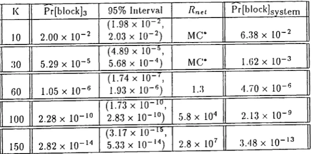
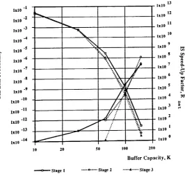
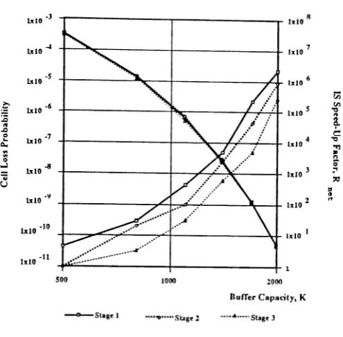
Figure 8: Estimated cell loss probabilities and IS speed-up factors, Rile!I as a function of the queue. capacity,

Fast Simulation

of

Queueing ... , Devct,sikiotis,

f\l-Qaq,

Fteebeteyset, ent! Townsend 26

5.2.3 Tile

SGD

Algorithrn for Tand em

M-IBP+MMBBP /D

/l/K Queues

Here, the estimate of the cell loss probability at the input of the ,S'-til stage in l.he tandem

network is obtained

by

using the SeD algorithm to minimize the estimate of the variance of the average number of tagged cells blocked per ItC at the S~-thstage with respect to the

IS bias

parameters. This requires that

S

stages be used to estimate the cell loss probability

at the input of the S-th stage.

The

average number

of

arrivals per RC is estimated using conventional

rvrc

sirnulation since arrivals are not rare events.

n.egelleration epochs are defined as the instants where each queue in the network is empty,

the ta.gged traffic stream is going active and gelleratillg a cell, and all the external traffic

streams in the network are idle. In each

Re,

qr, P«. and 'l» are initially biased to

q;~;),

P:~~),

q;'\S)

respectively, where s indexes the stage in the tandem network and

S

indexes the

position in the tandem network which is being optimized,until one customer is blocked, then

the IS parameters are changed to q;~;), ]J:~;),and q;,~S) in order to allow fast regeneration.

In these simulations,

q;~;)

=

qr,

P:~;)

=

n..

and

q;\S) =

qs,

and the optimization was

performed with respect to the settings of 01

=

q;~'i')

l

rr,

02s

=

]J:~;)

Ips, and 02s+1

=

q;\S)

/qs

for s

==

1, ... ,,5 using the SeD algorithm. In addition, each stage in the network was

assumed to have identical parameters, p

==

Ps, q

==

qs, and J(

==

!(s' The external traffic was not allowed to propagate through more than one stage

in

the tandem network. For the

example cases, the total offered ta.gged traffic load at each node was held fixed at 0.7, with

the offered external traffic load ranging from 0.5to 0.6. Table 7describes the system set-up

that was optimized for the example cases, referred to as systems 2 and 3 (consistently with

Section 5.2.2.) for 1, 2, and 3-stage tandem networks.

As with the single queue case, the SeD algorithm was applied by using as the starting

point the near-optimal biasing for a smaller queue capacity. Obtaining the near-optimal IS

biasing for shorter buffers was not difficult, since the corresponding cell loss probabilities

were high and the space could be searched efficiently with the SeD algorithm starting from

the brute-force

Me

point. Initially, this was done for the tandem configurations as well