Mining of uncertain Web log sequences with access history probabilities

University of Windsor University of Windsor

Scholarship at UWindsor

Scholarship at UWindsor

Electronic Theses and Dissertations Theses, Dissertations, and Major Papers

2010

Mining of uncertain Web log sequences with access history

Mining of uncertain Web log sequences with access history

probabilities

probabilities

Olalekan Habeeb Kadri University of Windsor

Follow this and additional works at: https://scholar.uwindsor.ca/etd

Recommended Citation Recommended Citation

Kadri, Olalekan Habeeb, "Mining of uncertain Web log sequences with access history probabilities" (2010). Electronic Theses and Dissertations. 8058.

https://scholar.uwindsor.ca/etd/8058

This online database contains the full-text of PhD dissertations and Masters’ theses of University of Windsor students from 1954 forward. These documents are made available for personal study and research purposes only, in accordance with the Canadian Copyright Act and the Creative Commons license—CC BY-NC-ND (Attribution, Non-Commercial, No Derivative Works). Under this license, works must always be attributed to the copyright holder (original author), cannot be used for any commercial purposes, and may not be altered. Any other use would require the permission of the copyright holder. Students may inquire about withdrawing their dissertation and/or thesis from this database. For additional inquiries, please contact the repository administrator via email

Mining of Uncertain Web Log Sequences

with Access History Probabilities

By

Olalekan Habeeb Kadri

A Thesis

Submitted to the Faculty of Graduate Studies through the School of

Computer Science in Partial Fulfillment of the Requirements for the Degree

of Master of Science at the

University of Windsor

Windsor, Ontario, Canada

2010

1*1

Library and Archives Canada

Published Heritage Branch

395 Wellington Street OttawaONK1A0N4 Canada

Bibliotheque et Archives Canada

Direction du

Patrimoine de I'edition

395, rue Wellington OttawaONK1A0N4 Canada

Your file Votre reference ISBN: 978-0-494-62717-4 Our file Notre reference ISBN: 978-0-494-62717-4

NOTICE: AVIS:

The author has granted a

non-exclusive license allowing Library and Archives Canada to reproduce, publish, archive, preserve, conserve, communicate to the public by

telecommunication or on the Internet, loan, distribute and sell theses

worldwide, for commercial or non-commercial purposes, in microform, paper, electronic and/or any other formats.

L'auteur a accorde une licence non exclusive permettant a la Bibliotheque et Archives Canada de reproduire, publier, archiver, sauvegarder, conserver, transmettre au public par telecommunication ou par Nntemet, prefer, distribuer et vendre des theses partout dans le monde, a des fins commerciales ou autres, sur support microforme, papier, electronique et/ou autres formats.

The author retains copyright ownership and moral rights in this thesis. Neither the thesis nor substantial extracts from it may be printed or otherwise reproduced without the author's permission.

L'auteur conserve la propriete du droit d'auteur et des droits moraux qui protege cette these. Ni la these ni des extra its substantiels de celle-ci ne doivent etre imprimes ou autrement

reproduits sans son autorisation.

In compliance with the Canadian Privacy Act some supporting forms may have been removed from this thesis.

Conformement a la loi canadienne sur la protection de la vie privee, quelques

formulaires secondaires ont ete enleves de cette these.

While these forms may be included in the document page count, their removal does not represent any loss of content from the thesis.

Bien que ces formulaires aient inclus dans la pagination, il n'y aura aucun contenu manquant.

AUTHOR'S DECLARATION OF ORIGINALITY

I hereby certify that I am the sole author of this thesis and that no part of this thesis has

been published or submitted for publication.

I certify that, to the best of my knowledge, my thesis does not infringe upon anyone's

copyright nor violate any proprietary rights and that any ideas, techniques, quotations, or

any other material from the work of other people included in my thesis, published or

otherwise, are fully acknowledged in accordance with the standard referencing practices.

Furthermore, to the extent that I have included copyrighted material that surpasses the

bounds of fair dealing within the meaning of the Canada Copyright Act, I certify that I

have obtained a written permission from the copyright owner(s) to include such

material(s) in my thesis and have included copies of such copyright clearances to my

appendix.

I declare that this is a true copy of my thesis, including any final revisions, as approved

by my thesis committee and the Graduate Studies office, and that this thesis has not been

ABSTRACT

An uncertain data sequence is a sequence of data that exist with some level of doubt or probability. Each data item in the uncertain sequence is represented with a label and probability values, referred to as existential probability, ranging from 0 to 1.

Existing algorithms are either unsuitable or inefficient for discovering frequent sequences in uncertain data. This thesis presents mining of uncertain Web sequences with a method that combines access history probabilities from several Web log sessions with features of the PLWAP web sequential miner. The method is Uncertain Position Coded Pre-order Linked Web Access Pattern (U-PLWAP) algorithm for mining frequent sequential patterns in uncertain web logs. While PLWAP only considers a session of weblogs, U-PLWAP takes more sessions of weblogs from which existential probabilities are generated. Experiments show that U-PLWAP is at least 100% faster than U-apriori, and 33% faster than UF-growth. The UF-growth algorithm also fails to take into consideration the order of the items, thereby making U-PLWAP a richer algorithm in terms of the information its result contains.

KEYWORDS

Uncertain data mining, frequent sequential patterns, Web log mining, existential

DEDICATION

To all those whom I had leaned on through my sojourn in life. This is

ACKNOWLEDGEMENT

My sincere appreciation goes to my parents, wife and siblings. Your perseverance and

words of encouragement gave me the extra energy to see this work through. Special

thanks go to Dr. A.O. Abdulkadri and family. Your financial and moral support is key to

seeing me through those challenging moments. I will forever be grateful.

I will be an ingrate without recognising the invaluable tutoring and supervision from Dr.

Christie Ezeife. Your constructive criticism and advice at all times gave me the needed

drive to successfully complete this work. The research assistantship positions helped as

well!!

Special thanks go to my external reader, Dr. Dilian Yang, my internal reader, Dr. Alioune

Ngom, and my thesis committee chair, Dr. Akshaikumar Aggarwal for accepting to be in

my thesis committee. Your decision, despite your tight schedules, to help in reading the

thesis and providing valuable input is highly appreciated.

And lastly to friends and colleagues at Woddlab, I say a very big thank you for your

TABLE OF CONTENT

AUTHOR'S DECLARATION OF ORIGINALITY Ill

ABSTRACT IV

DEDICATION V

ACKNOWLEDGEMENT VI

LIST OF FIGURES IX

LIST OF TABLES X

1. INTRODUCTION 1 1.1 Data mining approaches 1

1.2 Web mining types 2 1.3 Uncertain data sequence 3

1.4 Problems and applications of mining with dirty and uncertainty data 4

1.5 Thesis problem and contribution 11

2. RELATED WORKS 12 2.1 Apriori based methods 12

2.1.1 Apriori algorithm (AprioriAII) 13

2.1.2TheGSP algorithm 16 2.2 Pattern approaches 20

2.2.1 FP-growth algorithm 20

2.2.2 Freespan 22 2.2.3 PrefixSpan 25 2.2.4 The WAP mine algorithm 27

2.2.5 PLWAP algorithm 30 2.3 Uncertainty approaches for mining patterns 32

2.3.1 Trio system 33 2.3.2 Databases with uncertainty and Lineage 34

2.3.3 Working Model for uncertain data 37 2.3.4 U-apriori and local trimming, global pruning and simple-pass patch up

strategy (LGS) algorithm 40 2.3.5 UF-growth algorithm 43 3. PROPOSED MINING OF UNCERTAIN WEBLOG SEQUENCES WITH

ACCESS HISTORY PROBABILITIES 48 3.1 Observation on uncertain sequences 50

3.3 Building U-PLWAP algorithm 52 3.4 The U-PLWAP algorithm 53 3.5 Example of mining using U-PLWAP 60

4. COMPARATIVE ANALYSIS 71 4.1 Comparing U-PLWAP with U-apriori and UF-growth 71

4.1.6 Effect of varying length of sequence on memory use 78

4.2 Time complexity analysis 79 4.2.1 Time complexity of U-PLWAP 79

4.2.2 Complexity of U-PLWAP tree in terms of number of nodes 80

5. CONCLUSION AND FUTURE WORK 81

LIST OF TABLES

Table 1: Example of uncertainty in sequences 3 Table 2: Conditional functional dependencies 5

Table 3: The US-Census sample data 6 Table 4: The 4 different web log sessions 9 Table 5: The merged and sorted logs for the different sessions 10

Table 6: The generated uncertainty in the logs 10

Table 7: The sequence formed 13 Table 8: The sample transaction database 13

Table 9: The Large 1-sequence 14 Table 10: The transformed sequence 15

Table 11: L3 15 Table 12: C3 15 Table 13: L2 15 Table 14: C2 15 Table 15: L4 16 Table 16: C4 16 Table 17: The table explaining GSP algorithm 18

Table 18: The data sequence for candidate sequence check 19

Table 19: The sample database 20 Table 20: The FP-growth mining process 22

Table 21: The sample sequence database 23 Table 22: The frequent item matrix 23 Table 23: Pattern generation 24 Table 24: The sequence database 26 Table 25: The Projected database and frequent patterns 27

Table 26: The Web Access Sequence Database 28

Table 27: The Web Access Database 31 Table 28: The representation of uncertain data 33

Table 29: Models and their constraints 39 Table 30: Closure property of the incomplete model 40

Table 31: Sequence without probability 41 Table 32: Sequence with uncertainty 41 Table 33: The uncertain database 44 Table 34: The 4 different web log sessions 49

Table 35: The merged and sorted logs for the different sessions 49

Table 36: Uncertainty in sequences 50 Table 37: Sequence without probability 50 Table 38: Sequence with uncertainty 50 Table 39: Sample uncertain sequence mined with U-PLWAP 60

Table 40: U-apriori details for C3 70 Table 41: U-apriori details for C2 70 Table 42: The performance of U-PLWAP, UF-growth and U-apriori with different

Table 44: Comparison of U-PLWAP, UF-growth and U-apriori with different sequence

length 75 Table 45: Memory consumption of U-PLAWP, UF-growth and U-apriori with different

minimum support 76 Table 46: Memory size requirement for different data sizes 77

Table 47: Memory requirement of U-PLWAP, UF-growth and U-apriori with different

LIST OF FIGURES

Figure 1: The constructed FP-tree 21 Figure 2: The Web Access Pattern tree 28

Figure 3: |c 29 Figure 4: jac 29 Figure 5: The PLWAP tree with the header linkages 31

Figure 6: Hierarchies of the models 39

Figure 7: The UF-tree 45

Figure 8: |e 46 Figure 9: |de 46 Figure 10: The Existential Probability algorithm 51

Figure 11: The U-PLWAP algorithm 56 Figure 12: Frequentl-events algorithm 56 Figure 13: U-PLWAP_tree algorithm 57

Figure 14: Mine algorithm 59 Figure 15: The U-PLWAP tree after reading the first sequence 62

Figure 16: The U-PLWAP tree after the second sequence is read 63 Figure 17: The U-PLWAP tree after the third sequence is read 64 Figure 18: The U-PLWAP tree after the fourth sequence is read 65

Figure 19: The complete linked U-PLWAP tree 66

Figure 20: Conditional suffix tree o f ' a ' 68 Figure 21: Conditional suffix tree of'ab' 69 Figure 22: The graph comparing execution time of U-PLWAP with U-apriori when

minimum support values vary 72 Figure 23: The graph comparing execution time of U-PLWAP with UF-growth when

minimum support values vary 73 Figure 24: The graph comparing speed of U-PLWAP and U-apriori when data sizes vary

74 Figure 25: The graph comparing speed of U-PLWAP and UF-growth when data sizes

vary 74 Figure 26: The graph demonstrating the effect of varying the length of sequence on

U-PLWAP and U-apriori 75 Figure 27: The graph comparing speed of U-PLWAP with UF-growth when length of

sequences vary 76 Figure 28: The graph demonstrating the memory need PLWAP, UF-growth and

U-apriori with different minimum support values 77 Figure 29: The graph showing memory requirement for the 3 algorithms when data sizes

are varied 78 Figure 30: The graph demonstrating the memory requirement of the algorithms with

1. INTRODUCTION

Data mining or knowledge discovery is generally referred to as the process of analyzing

data from different views and situations and presenting it into useful information that can

be used to make critical decisions about day to day running of a business or process. This

process involves analysing data from many different dimensions or angles, categorizing

and summarizing the relationships identified with the aim of increasing revenue and/or

cutting time and costs of the processes represented by the data. Agrawal and Srikant

(1996) define data mining as a way of efficiently discovering interesting rules from large

databases. This area of study is motivated by the need to continuously look for solutions

to decision support problems faced by large retail organisations.

Data mining typically involves creating databases or warehouses where data are then read

using various techniques to analyse and forecast on future events. Algorithms that

employ techniques from statistics, machine learning and pattern recognition are used to

search large databases automatically. The process goes beyond simple data analysis.

Continuous innovations in computer processing power, disk storage, data capture

technology, algorithms and methodologies have all helped in realizing this objective. One

key factor that is important towards ensuring that information derived from data mining

is accurate is the use of broad range of representative data so that conclusions drawn from

data can be good enough to represent the general situation. Related to this is also the

aspect of ensuring proper cleaning is done on these representative data when required so

that accurate results are generated.

1.1 Data mining approaches

The process of discovering interesting information from huge set of data often employs

different techniques and approaches. Some of the approaches include:

• Classification

• Clustering

Classification involves arranging data into predefined groups. This is the filtering

technique used in grouping spam and non-spam mails. Some of the algorithms used here

are nearest neighbours, Naive Bayes classifier and neural network.

Clustering, like classification, also groups data into groups but using similarities that exist

between data rather than predefined grouping. K-means algorithm is an example that is

used with this approach. Regression method finds functions that model the data with least

error. Genetic programming is one of such techniques used for this purpose.

Association rule mining involves finding relationships that exist among data items in a

database. It involves finding patterns in the data items which are dependent on support

count and confidence values of the rules establishing relationships between data items.

Rules like if item A (antecedent) is purchased then item B (consequent) is also purchased

can be used to calculate the support count and confidence of "if A then B" as follows:

Support (A => B ) = number of occurrence of (A and B)/ Total number of transaction.

Confidence (A => B) = number of occurrence of (A and B)/ number of occurrence of (A)

The approach proposed in this research is based on this technique.

1.2 Web mining types

Web Mining is often referred to as the extraction of interesting and potentially useful

patterns and implicit information from the activity related to the World Wide Web. Three

categories in which web mining is usually viewed are:

• Web Content Mining

• Web Structure Mining

• Web Usage Mining.

Web content mining is the process of extracting knowledge from the content of web

pages, documents or their descriptions. Wrappers are used to map documents into some

models in order to be able to explore known structures in documents. Documents can

Web structure mining can be defined as the process of discovering knowledge from the

World Wide Web organization and links between references and referents on the Web.

Web structure mining involves making intelligent deductions from the links directed into

and out of contents on the web. This inward and outward links indicates the richness or

importance to which the content is to a particular topic. Counters attached to these links

can be used to retrace the structure of the activities on the web content.

Web Log Mining is the process of extracting interesting patterns in web access logs.

Since web servers record and accumulate data about user interactions whenever requests

for resources are received, such information can be collected, cleaned and analysed for

knowledge discovery. Information such as user behaviour as regards page visiting

patterns can be studied in order to aid the design and organisation of such websites. It can

also serve as attractive means of choosing where advertisements are placed on websites.

The web log can be taken a step further by dynamically customizing the order and

structure in which pages are displayed for each user based on their respective browsing

history.

1.3 Uncertain data sequence

An uncertain data sequence is a sequence of data that exists with some level of doubt or

probability. Each data item in the uncertain sequence is represented with a label and

probability values, referred to as existential probability, ranging from between 0 and 1.

This shows the level of assurance that an item exist in the sequence. A zero (0) value

indicates the item does not exist while one (1) shows that the item is 100% present in the

sequence. Table 1 gives an example of uncertain sequences.

UserJD

10

20

30

Table 1:

Uncertain sequence

(a:l,b:0.5,c:0.75,d:0.5)

(a:l,d:0.5,e:0.5,d:0.5)

(a:l,b:0.5,d:0.5,b:0.5)

UserJDD 10 for example, is represented by (a:l, b:0.5, c:0.75, d:0.5) indicating that item

'a' has 100% probability of existence. Items b, c and d however have 50%, 75%, and

50%o existential probabilities respectively.

The problem of mining frequent sequence in uncertain data sequence is that of

determining those sequences whose expected support count are greater than or equal to a

specified threshold called minimum support. The expected support of an uncertain

sequence is given by the sum of product of existential probability of the constituent items

of the sequence (Chui et al., 2007). For example, given the database as shown in table 1,

the expected support count of sequence 'ab' is calculated as (1 x 0.5) + (1 x 0.5) = 1. This

is then compared with a specified minimum support. If the minimum support is 1, the

sequence 'ab' is said to be frequent.

1.4 Problems and applications of mining with dirty and uncertainty

data

Cong et al. (2007) show that real world data often contain inconsistencies and errors. The

challenge is therefore in removing these errors (dirt) while ensuring the integrity of the

data is maintained. It is of high importance that the original meaning of the data is not, in

any way, changed. They demonstrate that the traditional functional dependencies in

database (Normal forms) may not fully guarantee the correct content of the database.

Given an order database shown as follows:

Order (id, name, AC, PR, PN, STR, CT, ST, zip). Each order contains name, unique item

id, and price (PR) of the item. It also contains the phone number, which contains area

code (AC) and phone number (PN), and the address that indicates street (STR), city (CT),

state (ST) and Zip code (Zip) of the customer buying the item. The functional

dependencies of the Order database are as follows:

fi[AC, PN]—• [STR, CT, ST] f2 [Id] — • [name, PR]

Where AC, PN, STR, CT, ST are Area Code, Phone Number, Street, City and State

respectively. Id represents the item identification number and PR is its price. This design

for example only specifies that AC and PN identify [STR, CT, ST] but fails to restrict

values that can be entered to represent real life situation. Area code 212 for example, can

be used to represent any city in the US. However in real life situation, 212 can only

represent New York City (NYC) as a city and New York (NY) as a state. A conditional

functional dependency (CFD) cp is then defined as ([AC, PN] —•[STR, CT, ST]), with an

additional constraint T defined on attributes of the table that stipulates the kind of values

that may exist together in the tables while still ensuring that each AC and PN uniquely

identify each STR, CT, ST combinations. An instance of the table showing the constraint

T is shown in Table 2:

AC -212 610 215 Tab PN

-e 2 : C STR -]ondit CT -NYC PHI PHI lonal fu ST -NY PA PA nctioi functional dependencies

With these additional constraint, all entries having 212 as AC must be from NYC and NY

while those from PHI and PA must either have 610 or 215 AC. Non conforming tuples

are cleaned accordingly.

Cong et al. (2007) stress that it is in order to guarantee the accuracy of cleaned data after

the application of data cleaning methodology, inspection of a manageable sample of the

cleaned data is needed. This ensures the accuracy of the repairs found is above a

predefined bound with high confidence. This is done by drawing a sample of K tuples

from the repaired database. A predefined inaccuracy threshold £, is specified. The sample

is partitioned into M strata where M< K. Each stratum is then assigned its inaccuracy

threshold ^i such that E,\ +^2 +...+ ^M = 1- Each ^i can be adjusted depending on the

likelihood that inaccurate tuples may exist in a particular stratum. The number of tuples

drawn from each stratum is given by the product of ^i and K (total number of tuples). The

The ratio of number of tuples in stratum i to the number of tuples drawn from the stratum

to check for inaccuracy is defined by Sj = Pj / (^ . K).

The inaccuracy rate, p = (Xei . Sj) / (£Pj . Si ), where Pj is the number of tuples in each

stratum i.

The test statistic z = (p - £,) / (V(£(l - £,)/K)) where p is the inaccuracy rate of the sample

The test statistic z is tested against the critical value zx at confidence level 5. If z < - zx ,

inaccuracy level of the cleaned data is said to be below the threshold £, making the

cleaned data acceptable for use.

Chiang and Miller (2008) go a step further by automatically generating conditional

functional dependencies (CFDs) for a given relation with sample data. These CFDs are

then used to remove the dirty data that fail to comply with the CFDs without any need of

human inspection. Given the relation showing US Census Data:

Tuple ti t2 t3 t4 t5 t6 t7 t8 t9 tio tn CLS Private Private Self-emp ? Self-emp Never-worked Self-emp Local-gov State-gov ? Self-emp ED Bachelors Bachelors Masters HS-grad Masters 7m-8th

HS-grad Some college Masters Bachelors Some college MR Married Married Married Divorced Married Divorced Never-married Never-married Divorced Divorced Never-married

occ

Exec-mgr Prof-specialty Exec-mgr ? Admin ? Farming Admin Prof-specialty ? Machine-up REL Husband Husband Wife Not-in-family Wife Not-in-family Own-child Own-child Own-child Not-in-family Not-in-family GEN Male Male Male Male Female Male Male Female Male Female Female SAL >50K >50K >50K >50K >50K <50K <50K <50K >50K <50K >50K

The CFDs are generated by partitioning a relation into attributes of equivalence classes.

CFDs are then defined between classes X—•Y when there exist some classes in X that are

fully contained in some classes in Y. The CFDs are then defined on the conditions in

which the classes are contained in each other. If for example, the following classes,

denoted by n , are defined from the census sample data based on the similarities in their

values:

nM R= {{1,2,3,5}, {4,6,9,10}, {7,8,11}}

nREL= {{1,2}, {3,5}, {4,6,10,11}, {7,8,9}}

n(R,M) = {{1, 2}, {3, 5}, {4, 6, 10}, {7, 8} {9}, {11}}

nE D - {{1, 2, 10}, {3, 5, 9}, {4, 7}, {6}, {8, 11}}

ricLS = {{1, 2}, {3, 5, 7, 11}, {4, 10}, {6}, {8}, {9}}

n(C,E)= {{1,2}, {10}, {3,5}, {4}, {6}, {7}, {8}, {9}, {11}}

n(M,E)= {{1, 2}, {10}, {3, 5}, {4}, {6}, {7}, {9}, {8, 11}}

n(M)E,c)= {{1,2}, {10}, {3,5}, {4}, {6}, {7}, {9}, {8}, {11}}

The class TIMR is formed by grouping tuple numbers with same value in column MR.

That of ri(c,E) is formed by grouping tuples with same value in both CLS and ED and so

on. Rules are then formed by establishing edges between classes. For edge

X—•Y = (REL —•(REL, MR)). The classes {1,2}, {3,5} in REL are also contained in

(REL, MR). REL is then conditioned on common values in {1,2} and {3, 5} to give the

CFDs required. The CFDs are: ({REL = 'Husband'}__• MR) and

({REL = 'Wife'} —•MR) or more explicitly as ({REL = 'Husband'} — • Married) and

({REL ='Wife'} —> Married).

By going to the next level, when the 'X' part of the edge has more than an attribute, one

of the attributes is made the conditional attribute if a match is found.

If X—*Y = (ED, MR)—•(ED, MR, CLS)). The classes {1, 2} and {3, 5} in (ED, MR) is

contained in (ED, MR, CLS). If MR is made the conditional attribute from (ED, MR), a

class in nMR that only contains tuples from {1,2} and {3, 5} must be found in order to

value in {1,2,3,5} = Married. Therefore, the rule: ({MR = 'Married', ED} — • {CLS}).

This means that MR must be married for MR and ED to functionally determine CLS.

The main problem with dirty data is being able to strike a balance between making sure

dirty data are not used for mining and at the same time ensuring the cleaning process does

not introduce another set of unwanted data. While the Cong et al. (2007) approach needs

sampling and physical inspection to guarantee its correctness, the automatic approach of

Chiang and Miller (2008) depends on the cleanliness of the data that is used to generate

the rules.

In recent times, there has been interest in mining data generated from non-traditional

domains such as sensor networks and location based services. Such data are generated

with some level of uncertainty due to measurement inaccuracies, sampling error and

network latencies. Location based systems as found in GSM (Global System for Mobile

communication) are used in delivering several value added services in the mobile

telephoning industry. It can be used in determining location of a subscriber or the nearest

banking cash machine. However, due to the unreliability of radio signal that is used to

relay information from the nearest mobile base station (tower), information delivered

might sometimes be prone to errors. Fluctuations in signals and network can cause some

farther base stations to serve a particular mobile subscriber and as a result deliver

information on a farther location. Therefore mining data generated by such systems

demands attaching some uncertainties unto them.

Sensor networks that combine computational functionalities with physical sensing

capabilities could also transmit errors of the physical entity such as temperature that they

are designed to measure. Sensors designed to capture temperature values might be

corrupted or biased if placed near a power generating plant or an air conditioner. Analysis

based on these types of data may therefore be inaccurate if the uncertainties that may be

One main problem associated with mining uncertain data is how such data are objectively

generated. Chui et al. (2007) and Leung et al. (2008) also suggested that historical

behaviour of entities can be used for presenting uncertainties that might be attached to

their current behaviour. Their work does not show exactly how this can be done

objectively. The use of historical data can be used objectively in arriving at a more

unbiased result during mining based on sample data. Uncertainties can also be useful in

analysing how unique users may find a particular webpage useful. Such analysis can then

be used in improving the design of such websites. Web logs, though are doubtless facts,

can be represented with uncertainty when history of log sessions for each user is used to

compute the consistency of the user's behaviour based on the most current web log

session.

Given four different web log sessions as shown in Tables 4a, 4b, 4c and 4d. The tables

represent access histories for users 10, 20 and 30 at different times 1, 2, 3 and 4. User IDs

10 and 30 participates in all the 4 sessions while user ID 20 only take part in twice. The

most current session is time 4. The four web log sessions are then merged into one

database and ordered by user ID and time so that the most current web log for each user

comes first as shown in Table 5.

User ID 10 20 30 Time 4 3 2 1 2 1 4 3 2 1 Web logs (a,b,c,d) (a,d,a,b) (a,d,c,a) (a,c,a,c) (a,d,e,d) (a,c,b) (a,b,d,b) (a,c,e,b) (a,e,d,e) (a,e)

Table 5: The merged and sorted logs for the different sessions

The existential probability, prob (u(e)), of each event e, for each user u, in the most

current log is given as: Number of existence of e in any record with u prob (u(e)) =

Total number of records with u

The likelihood of having the latest log to be a true reflection of how each user browses

the site based on the historical behaviour is calculated as follows:

User ID 10: Since 'a' appears at least once in all the 4 logs, existential probability of 'a'

is given as 4/4 = 1. Item 'b' appears only in the first two logs, its existential probability is

2/4 = 0.5. Item 'c' appears 3 times, its existential probability is 3/4 = 0.75 and that of d is

2/4 = 0.5. Using the same method, user ID 20's existential probability values for the

latest log is:

'a' = 2/2 = 1

'd' = 1/2 = 0.5

'e' = l/2 = 0.5

User ID 30:

'a' = 4/4 = 1

'b' = 2/4 = 0.5

'd' = 2/4 = 0.5

The uncertain sequence to be mined is therefore given as in Table 6 :

UserlD 10 for example, is represented by (a:l, b:0.5, c:0.75, d:0.5) indicating the

consistency of the current behaviour based on the historical behaviour. There is a 100%

certainty that U s e r l D 10 always visit page 'a'. In the same manner, the probability of

pages b, c, d are 50%, 75%, and 50% respectively.

1.5 Thesis problem and contribution

This thesis is set out to propose a sequential web log mining solution for mining

uncertain weblog sequences with access history probabilities using the PLWAP tree

mining approach. The works of Agrawal and Srikant (1995), Pei et al. (2000) and Ezeife

and Lu (2005) are all based on precise data sequences with 100% certainty. Chui et al.

(2007) proposed U-apriori, an uncertain data implementation of apriori algorithm. Leung

et al. (2008) proposed UF-growth that is a non-sequential mining approach of frequent

patterns. The contributions of this thesis are therefore as follows:

• The approach (U-PLWAP) is the first tree based sequential mining approach for

data with uncertainty.

• U-PLWAP makes use of historical web log session in calculating existential

probability of web log sessions.

• The speed of the algorithm is improved by collapsing events with the same label

but different existential probabilities into one single node during the construction

of the U-PLWAP tree. This makes the U-PLWAP tree more scalable in terms of

number of nodes.

• In order to effectively mine frequent patterns in U-PLWAP, sequence of

cumulative products of existential probabilities of events found along each

temporary root nodes (from the root node) are dynamically generated for each

new sets of temporary root nodes.

• The general performance of U-PLWAP is at least 2 times faster than U-apriori.

The U-PLWAP algorithm is also at least 33% faster than UF-growth. This is

addition to the richer result generated by U-PLWAP (frequent sequential patterns)

2. RELATED WORKS

There have been several research findings on the general area of data mining. Specifically,

the problem of mining web logs can be traced back to the association rule mining

technique originally introduced by Agrawal and Srikant (1995). Etzioni (1996) state that

web mining can be useful for server performance enhancements, restructuring of website

and direct marketing in e-commerce. This has made research in this area an important

one, given the role internet and websites play in our day to day activities. Web log mining,

synonymous with Web usage mining, is one of the three areas of web mining identified

by Madria et al. (1999) and Borges and Leven (1999). Technically, the problem of

sequential mining of web logs is that of finding all ordered sequence of web pages

accessed whose support count is greater than a specified minimum threshold (Ayres et al.,

2002). Cooley (2003) defined web usage mining as "the application of data mining

techniques to web click stream data in order to extract usage patterns". Han and Kamber

(2006) also gave an insight to the area of data mining including the sequential mining of

web logs.

The discussion in this chapter is grouped into those methods that are apriori and

pattern-based. The algorithms with uncertainty are also discussed in a separate section.

2.1 Apriori based methods

This section gives an introduction into the problem of sequential pattern mining and the

early methods used to solve this problem. It gives insight into the general problem of

sequential mining which can be adapted to the web usage mining environment.

Agrawal and Srikant (1995) introduce the problem of mining frequent sequential patterns.

They state that early works by Agrawal et al. (1993) only concentrate on discovering

patterns within transactions. Agrawal and Srikant (1995) introduce and addressed the

problem of discovering sequential patterns in transactional databases where transactions

rather than treating items as a unit. For example, itemsets ((1,5) (2) (3) (4,7)) can be

considered for a single user or customer in the approach introduced by Agrawal and

Srikant (1995). That is, more than one itemset per record/user is considered for mining as

against single itemset per user in Agrawal et al. (1993).

2.1.1 Apriori algorithm (AprioriAll)

Agrawal and Srikant (1995) propose AprioriAll algorithm to discover sequential patterns

in a transaction database. The algorithm finds sequential patterns in transaction database

where several transactions can be done by a given customer as shown in Table 8. Such

transactions are grouped to form a sequence for each customer as given in Table 7.

Cust Id 1 1 1 1 2 2 2 2 3 3 3 3 4 4 4 5 5 Time 1 2 3 4 1 2 3 4 1 2 3 4 2 3 4 1 2 Transaction 1,5 2 3 4,7 1,8 3 4 3,5 1 2 3 4 1 3 5 4 5 Cust id 1 2 3 4 5 Sequence <(1,5)(2)(3)(4,7)> <(1,8)(3)(4)(3,5)> <(1) (2) (3) (4)> <(D(3)(5)> < (4) (5)>

Table 7: The sequence formed

Table 8: The sample transaction database

The sample transaction in Table 8 shows transactions done by each customer at different

time. The transactions are then grouped by customer ID so that customer ID 1 for

example has a sequence of transactions ((1,5) (2) (3) (4,7)) as shown in table 6. Each

transaction grouping in a sequence is known as itemset. For example, ((1,5) and (2) are

the minimum support must be specified. The database is then scanned to record the

occurrence of each itemset in order to discover if such itemset is frequent. Itemsets with

count that is greater or equal to the minimum support are said to be frequent. The set of

frequent itemsets are referred to as the Large itemsets. Given the sequence shown in

Table 8, the algorithm operates in 5 phases; Sort phase, Litemset (Large itemset) phase,

Transformation phase, Sequence phase and Maximal phase.

The sort phase prepares the transaction database by grouping transactions according to

the customer ID thereby forming a sequence for each customer ED. Using the sequence in

Table 8, AprioriAll works by first ordering the transaction database by customer ID and

time. It is then implicitly changed to the form shown in Table 7. Given that the minimum

support is 2, the Large itemset phase then finds all frequent (Large) 1-sequences by

scanning the database for itemsets that occur more than once provided that the minimum

support specified is 2. Out of the possible itemsets (candidate itemsets) {(1), (2),(3), (4),

(5), (1,5), (1,8), (3,5) and (4,7)}, the frequent 1-sequences are as shown in Table 9.

1-Sequences (1) (2) (3) (4) (5)

Support 4 2 4 4 4 Table 9: The Large 1-sequence

Transformation phase is done by removing the non-frequent items/itemsets. It also

replaces all transactions with the set of all Large itemsets contained in that transaction. A

mapping of the transformed database is also shown in Table 10 given that large itemsets

(1). (2), (3), (4) and (5) are mapped to 1, 2, 3, 4, 5 respectively. Items 7 and 8 are not

Custid 1 2 3 4 5 Sequence Before Transformation <(1,5)(2)(3)(4,7)> <(1,8)(3)(4)(3,5)> <(1) (2) (3) (4)>

<(D 0 ) (5)>

<(4) (5)>

Sequence After

Transformation (deleting small items)

<{(1),(5)} {(2)} {(3)} {(4)}> <{(!)} 1(3)} 1(4)} f(3),(5)» <{(1)} {(2)} {(3)} {(4)}> <f(l)} {(3)} {(5)}> <{(4)} {(5)}> Table 10: The transformed sequence

The Sequence phase performs an apriori-gen join on the frequent 1-sequence in Table 9

to form candidate sequence C2 as shown in Table 14. Large 2-sequences (L2) are then

derived from C2 by selecting those with support greater than or equal to 2 since the

minimum support is 2. L2 is then used in an apriori-gen join to generate C3. Apriori-gen

join works by performing a self join on Lk-i in order to arrive at Ck only when the first

k-2 items are equal. The generated Ck is then pruned by removing any sequence in Ck

that has any of its k-1 subsequence not in Lk-i. For example, C3 is derived by an

apriori-gen join on L2 when the first items in each L2 are the same. That is, (12) joins with (13)

to form (1 2 3) because they both have ' 1 ' as the first item. C3 is then pruned by

removing any sequence that has any of its 2-subsequences not in L2. For example,

sequence (1 3 2) is pruned from C3 since its sub-sequence (3 2) is not in L2. This process

is recursively done to generate new Ck and I* until no more Ck is formed or no frequent

sequence found. The Tables 11 to 16 show the process in details.

Seq (12) (13) (14) (15) (2 3) (2 4) (2 5) (3 4) (3 5) (4 5) Count 2 4 3 3 2 2 0 3 2 2 Seq (12) (13) (14) (15) (2 3) (2 4) (3 4) (3 5) (4 5) Count 2 4 3 3 2 2 3 2 2 Table 13: L2

Seq ( 1 2 3 ) (12 4) (12 5) (13 4) (13 5) (14 5) (2 3 4) (3 4 5)

Count 2 2 0 3 2 1 2 1 Table 12: C3

Seq ( 1 2 3 ) (12 4) (13 4) (13 5) (2 3 4)

Supp 2 2 3 2 2 Table 11: L3

Seq (12 3 4) (13 4 5)

Count 2 0

Seq (12 3 4) Table 15:

Count 2 L4 Table 16: C4

Maximal phase is then executed by finding only frequent itemsets that are not contained

in any other large itemset. Itemsets {(4 5), (1 3 5), (12 3 4)} are not contained in any of

the large sequences. The maximal sequences are therefore {(4 5), (1 3 5), (12 3 4)}.

2.1.2 The GSP algorithm

Srikant and Agrawal (1996) introduced GSP, a more flexible approach into their earlier

work stated above. They show that the problem of discovering sequential patterns with

earlier approaches fail to take into account time constraints in the sequence to be

considered. They also stress that existing approaches have rigid definitions of

transactions. Grouping of items into hierarchies (taxonomies) can also be found to be

missing in the earlier algorithms. The authors proposed GSP (Generalized Sequential

Patterns) to cater for these limitations. The GSP algorithm is made more flexible by

including time constraints, flexibility in the definition of transaction and inclusion of

taxonomies. The time constraint is used to further extend the flexibility of the algorithm

by specifying the time limit within which a particular pattern can be considered frequent.

The flexibility in transaction definition also introduces the freedom to regroup

transactions based on a specified time interval within which transactions can be combined

into one unit (one itemset). This specified time is referred to as the sliding window. The

inclusion of taxonomy helps in further showing the hierarchy along which a frequent

pattern can be expressed. The example below shows the transactions of books sold in a

Sequence-Id

CI

CI

CI

C2

C2

C2

Transaction

Time

1

2

15

1

20

50

Items

Ringworld

Foundation

Ringworld Engineers, Second Foundation

Foundation, Ringworld

Foundation and Empire

Ringworld Engineers

Taxonomy T

Asimov Niven

Foundation Foundation Second Ringworld Ringworld

and Empire Foundation Engineers

Example 2.1 The example demonstrating additional functionalities of GSP algorithm.

If the minimum support is specified as 2, the frequent 2- element patterns are:

{(Ringworld) (Ringworld Engineers)} and {(Foundation) (Ringworld Engineers)}.

However, when a sliding window of 7 days is given, the pattern

{(Ringworld) (Ringworld Engineers)} also becomes frequent since the first 2 transactions

of CI becomes one transaction. Setting a maximum constraint of 30 days generates no

2-element frequent pattern since Ringworld Engineer in C2 was bought after the 30-day

limit.

Frequent patterns can also be expressed in form of their taxonomies. For example,

patterns supporting {(Foundation) (Ringworld Engineers)} will also support {(Asimov)

(Niven)}. This is made possible by also specifying the taxonomy as part of the input data.

For example, {(Foundation) (Ringworld)} will be represented as {(Foundation,

The GSP algorithm is a multiple-pass solution. The first pass considers the items

individually and generate the frequent 1-sequence for those with support count greater

than the minimum support. The 1-itemset (Li) is used to generate the next set of

candidate sequences (C2) by a join operation with itself. Subsequent Ck are generated

from Lk-i. A join operation (apriori gen join) is carried out only when the subsequence

generated by removing the first item in sequences in L^.i is the same as removing the last

item during the self join on Lk-i. The candidate sequences are searched for using the

forward and backward phase algorithm. Pruning operation is also performed to remove

those candidate sequences whose k-1 contiguous sub-sequences are not frequent. The set

of Lk sequences are then generated. The algorithm ends when there are no more

sequences generated in Lk .

Using Table 17 as an example, frequent 3-sequences is self joined using the apriori gen

join which states that a join can only occur if by removing the first item in sequences in

Lk-i , the subsequence left is the same as removing the last item during the self join on

Lk-i. For example, sequence ((1,2) (3)) joins with ((2) (3,4)) since the last 2 items (2,3) in

the first sequence and the first 2 items (2,3) in the second sequence are the same. Equally,

((1,2) (3)> joins with ((2) (3) (5)>. The join operation then produces ((1,2) (3,4)> and

((1,2) (3) (5)). Sequence ((1,2) (3) (5)) is however pruned since its contiguous

sub-sequence ((1,2) (5)) is not frequent (not in frequent 3-sub-sequence).

Frequent 3-Sequences

( ( 1 , 2 ) ( 3 ) ) < (1, 2) ( 4 ) )

< W ( 3 , 4 ) )

{ ( 1 . 3 ) ( 5 ) ) {(2) ( 3 , 4 ) ) < ( 2 ) ( 3 ) ( 6 ) >

Candidate 4-Sequences after join

( ( 1 . 2 ) (3. 4 ) ) ( ( 1 , 2 ) (3) ( 5 ) )

after pruning ( ( 1 , 2 ) ( 3 , 4 ) )

The GSP algorithm checks for candidate sequence in 2 phases; the forward and backward

phase. The forward phase finds successive elements of candidate sequence in a sequence

databases given that the difference between the start time of the new element and the end

time of the previous element is within the maximum time (constraint) specified. When

the difference is more than the maximum time, the algorithm calls the backward phase. If

no element(s) is found in this phase, the sequence database does not contain the candidate

sequence.

The backward phase backtracks and checks the previous elements. This is to ascertain

that no occurrence of the immediate previous element has its start time earlier than the

difference between end time of the present element and the maximum gap constraint. The

backtracking continues until such an occurrence is found or the very first element of the

candidate sequence is pulled up. A new set of elements are then searched with the

forward phase starting from the last point of backtrack.

Transaction- Time

10

26

45

50

65

90

95

Items

1, 2

4, 6

3

1, 2

3

2 , 4

6

Table 18: The data sequence for candidate sequence check

If Table 18 is used as an example with maximum gap of 30, minimum gap of 5 and

window size 0. Candidate sequence <(1, 2) (3) (4)> can be searched by first finding (1, 2)

at transaction time 10 and then (3) at time 45. Because the time between the 2 elements is

35 days (greater than max gap of 30), element (1, 2) is pulled up by the backward phase

of the algorithm. The first occurrence of (1, 2) with transaction time after 15 (45 - 30) is

searched for. Since no such element exists and the first element in the candidate sequence

is pulled up already, the forward phase continues with a fresh search of the candidate

found at 65. Since the gap between these two elements is within thin the minimum and

maximum gap, the next element (4) is then found at transaction time 90

Which is also within the maximum gap relative to immediate past element (3) found at

time 65. Therefore the data sequence shown in Table 18 contains the candidate sequence

<(1, 2) (3) (4)> under the conditions stated.

2.2 Pattern approaches

2.2.1 FP-growth algorithm

Han et al. (2004) aim at solving problem of candidate set generation during frequent

pattern mining process. They found that candidate set generation can be costly especially

when many patterns are present and when such patterns are long.

Han et al. (2004) proposed a frequent mining algorithm, FP-growth, based on frequent

pattern tree (FP-tree) data structure. Through this, the authors contributed to the study by

ensuring large database is compressed into FP-tree therefore removing repetitive database

scan. This divide and conquer, conditional mining approach also remove candidate set

generation.

The FP-tree is built on the intuition that if frequent items are used to re-order items in the

database, multiple transactions sharing same itemset can be represented with the same

path in FP-tree by registering their counts. FP-tree is constructed after a first scan of the

database is carried out where frequent items are found and ordered. The order is then

used to enter items into the FP-tree during the second scan. Given the database below:

TID

100 200 300 400 500

Items Bought

/ , a,c,d}g, i, tn-,p

a,h,c,f, f , m , 0 b,f,h,j}o

b,c,k, s,p

a , / , c, <s,Z,p, m,n

(Ordered) Frequent Items

f,c,a,m,p

/,c?a,fo, m

f\b

It is assumed that the minimum support is 3. The items are re-ordered according to

descending order of frequent items (f:4, c:4, a:3, b:3, m:3, p:3). Items h, I, j , k, 1 have

been removed from the database since they are not frequent.

The items are then inserted into the FP-tree in the ordered fashion, registering the count

on each occasion. A header link table is also constructed to show the order in which

nodes of same type are inserted in order to aid mining process. The FP-tree generated is

as given below:

Figure 1: The constructed FP-tree

The mining process is done by starting from the bottom of the header table. Item p has 2

tree paths f:4, c:3, a:3, m:2, p:2 and c:l, b:l, p:l. Removing p and ensuring only counts

for item p are present gives p's conditional base tree: f:2, c:2, a:2, m:2, and c:l, b:l. Only

item c make the minimum count of 3 (sum), therefore forms p's conditional FP-tree (c:3).

Pattern 'cp:3' is therefore frequent. The process is then repeated for all items on the

header table. The conditional FP-tree is repeatedly mined when more then one frequent

Items P m

b a c f

Conditional pattern base (f:2,c:2,a:2,m:2), (c:l,b:l) (f:2, c:3,a:2),

(f:l,c:l,a:l,b:l)

(f:l,c:l,a:l),(f:l),(c:l) (f:3,c:3)

(f:3)

-Conditional FP-tree c:3

f:3, c:3, a:3

-f:3, c:3 f:3

-Final Frequent pattern cp:3

am:3, cm:3, fm:3, cam:3, fam:3, fcam:3

-ca:3, fa:3, fca:3 Fc:3

-Table 20: The FP-growth mining process

This approach is however limited to finding frequent patterns in non-sequential data.

2.2.2 Freespan

Han et al. (2000) proposed FreeSpan in order to solve the problem of sequential pattern

mining. It also removes some of the drawbacks of Apriori algorithm including, several

scan of the database, generation of huge candidate sequences and difficulty associated

with long sequential patterns.

The authors' approach is based on the integration of frequent pattern approach with that

of sequential patterns and uses projected databases to limit the search and growth of

subsequence fragments. Han et al. (2000) contributions include design of frequent item

matrix where frequent length 2-sequences are discovered. The authors also defined how

generation of item repeating patterns and projected databases for each frequent item are

found.

The algorithm works by using the first scan to generate the frequent items arranged in

order on f-list. The second scan of the database then generates the frequent item matrix.

From the matrix, the frequent 2-length sequences are noted. The sequences corresponding

to the frequent diagonal elements are noted in the annotation for repeating items. Other

non-diagonal sequences are also noted when the equivalent diagonal elements of the

scanned the third time to generate the final item repeating patterns and the projected

databases.

Given the sequence database as shown below:

Sequence-id

id

20 30 40 50 Sequence ((bd)cb(ac)} MHceMfg)) ({ah)(bf)ab/) <(*e)(«)d> (a(bd)bcb(ade))

Table 21: The sample sequence database

The frequent item list are generated and ordered as follows: (b:5, c:4, a:3, d:3, e:3, f:3). A

6x6 frequent item matrix is then formed with the frequent items. A triangular matrix is

then formed since half of the matrix is similar. The diagonal elements have one value

while other cells have three values with the first two representing the count of the

constituent items in the database when their positions are noted while the last value

represents the count when they both occur together. Table 22 represents this.

b c a d e / 4 (4,3,0) (3,2,0)

I £t, *•', M f | d , i , 1 } (2,2,2) b 1 (2,1,1) (2,2,0) (1,1,2) (1,1,0) c 2 (1,2,1) (1,0,1) (1,1,0) a 1 (1,1,1) (0,0,0) d 1 (1,1,0) e 2 /

Table 22: The frequent item matrix.

Taking the example of the second cell on the first column (4,3,0). This means (b,c)

occurs 4 times, <c,b> 3 times and 0 means both <(b,c)> never occur together at a time. The

frequent length 2 sequences, annotation on repeating items and annotation on projected

Item f e d a c b

Output length-2 sequential pattern

<bf):2,<fb>:2,<(bf)>:2 <be):3,<(ce)>:2,

<bd>:2, <db>:2, <(bd)>:2, <cd>:2, <dc>:2, <da>:2,

<ba>:3, <ab>:2, <ca>:2, <aa>:2, <bc>:4, <cb>:3

<bb>:4

Ann. on repeating items

{ b+f } <b+e>

{b+d},<da+>

<a a+>, {a+ b+} (d a+> {b+c}

<bb+>

Ann. On projected DB

-<(ce)>: {b} <da):{bc}, {cd}:{b} <ca>:{b}

-Table 23: Pattern generation

The length 2-sequential patterns are those entries that are greater than or equal to

minimum support of 2. Since F[b,b] and F[f,fJ are frequent, b and f can be repeated in as

many times as possible (+) and in any order ({}) as shown in the annotation for repeating

item column. Since no other frequent item exist with f apart from b, the annotation for

projected database is null. For the second row (e), F[e,e] is infrequent, as a result e is not

a repeating item as shown <b+,e>. Angular bracket is also used to restrict order of the item

since only one of the 3 values of (b,e) on the item matrix is frequent (3,1,1). Set notation

({}) is used if otherwise to indicate that both (b,e) and (e,b) are frequent.

The items on row 2 also form a triple F[c,e], F[b,e], F[b,c]. Set {b} is therefore included

in the projected database with the annotation containing c and e. In this case, <(ce)> is

used since it is the only frequent annotation. The third database scan is then done using

the item repeating annotation and projected database as guide to obtaining frequent

sequential pattern of longer length. The mining operation is then restricted to the patterns

contained in the projected database header set. The frequent patterns obtained in the third

scan are as follows: {<bbf>:2, <fbf>:2, <(bf)b>:2, <(bf)f>:2, <(bf)bf>:2, <(bd)b>:2, <bba>:2,

<aba>:2, <abb>:2, <bcb>:3, <bbc>:2}. There might be need to construct a new frequent item

matrix for projected databases whose annotation contains more than 3 items and

recursively mine its sequential pattern.

2.2.3 PrefixSpan

A sequence database is one that records events in its database in the order in which they

occur. As a result, it takes into account the time at which events occur. For example, the

sequences (abc) is different from (bac). Though both sequences contain the same

item/events, event 'a' comes before event 'b' in the first sequence and vice versa in the

second sequence. Therefore, in sequence databases, the two sequences are regarded as

two different sequences. Sequence of transactions can also be represented in the order in

which they occur and at the same time indicate events of the same transaction. For

example, the sequence (a(abc)(ac)d(cf)> contains (a), (abc), (ac), (d) and (cf) transactions

(elements) that occur separately in the order shown.

The Prefix-Projected Sequential Pattern Mining (PrefixSpan) by Pei et al. (2004) is

designed to solve the problem of mining sequential pattern. The approach uses a divide

and conquer method by projecting the sequence database over common frequent prefixes

and recursively mining each projected database. A prefix of a sequence is the part of a

sequence that strictly precedes it. For example, sequences (a), (a(ab)), (a(abc)) are

prefixes of sequence (a(abc)(ac)d(cf)>. On the other hand, sequences (ab> and (a(bc)) are

not.

The algorithm works by first making a scan on the database to find the frequent

1-sequential patterns. The database is then divided into n projected databases, defined by

sequences starting with each of the n 1-sequaential database. Each of these projected

databases are then recursively mined by further projection to determine the frequent

patterns they contain. Given the database as shown in Table 24 and minimum support of

2, the database is scanned to generate the frequent 1-sequentila pattern: a:4, b:4, c:4, d:3,

Sequencaid

10

20

30

40

Sequence

{a(abc)(ac)d(cf))

{(ad)c(hc)(m}) .

((ef){ab)(4f)d>)

'

(eg(af)cbc)

Table 24: The sequence database

The sequence database is then divided into 6 parts (6-projected databases) based on

sequences preceded by each of the frequent 1-sequential patterns. The second column of

Table 25 depicts this. A-projected database is found for example, by scanning the

database to find all sequences prefixed by 'a'. The first 2 sequences with sequence_ids 10

and 20 are preceded by 'a'. The sequences (a (abc) (ac) d (cf)> and ((ad) c (be) (ac))

minus 'a' forms their respective projected sequences ((abc) (ac) d (cf)> and ((-d) c (be)

(ac)). The sequence ((ef) (ab) (df) (cb)) is preceded by 'a' at element (ab). Element (ei) is

removed and the a-prefix sequence formed is ((-b (df) (cb)). The same method is used to

complete column 2 of Table 25.

Each projected database is then recursively mined by projection to discover any possible

frequent pattern. The a-projected database is for example, mined to discover if another 'a'

is frequent. The a-projected database shows that a is frequent (a:2) thereby making (aa) a

frequent pattern as shown in column 3 of Table Table 25. The resulting aa-projected

database found from a-projected database is {((-bc)(ac)(d)(cf)), ((-e))}. No further

frequent item can be found from this, therefore no frequent pattern prefixed by 'aa' can

be found. The algorithm, in the same manner, mines for ' b ' from a-projected database to

check if (ab) is frequent. Item ' b ' is found 4 times, making (ab) frequent. The resulting

projected database is ((-c) (ac) (d) (cf)), <(-c)(ae)>, ((c)), Recursively mining the

The same process is used for all the projected databases to find the respective frequent

patterns shown in Table 25. The union of these frequent patterns gives set of frequent

patterns for the database.

prefix

<«}

(6)

(c) (d) (e)

if)

projected (suffix) d a t a b a s e

((ahc)(ac)d(cf)), <(_<i)c(6c)(a«)>,

« J 0 ( # ) < * > , ((-f)cbc)

<(.x)Cac)d(c/)>, <(-c)(oe)>, <(d/)e&), (c)

((ac)d(cf)), ((bc)(ae)), (6}t <fec) ( ( c / » , (c(bc)(ae)), (U)cb)

(U){ab)(df)cty, ((af)cbc)

((ah)(df)cb), (cbc)

sequential p a t t e r n s

(a), (aa), (ah), (a(bc)), (a(bc)a), (aba), (abc), <(afe)), <(aft)c), ((a6)d), <(o6)/>,

{(a6)dc), (ac), (aca), (ocb), (occ), (ad),

{adc), ( a / )

<6>, (6o>, <*c>, ({be)), <(fcc)a), <M), (Mc),

<e>, <c«), <c6), (cc) <d>, (db), (dc), (deb)

(e), (ea), (eab), (eac), (each), (eb), (ebc),

H . <«*), <c/>, <e/6), (e/c>, (e/d»>.. </>. </6>,- </««), ( / c ) , (fob)

Table 25: The Projected database and frequent patterns

The technique has removed the need to generate candidate sequences during mining. It

also results in shrinking of projected databases as the mining process progresses. The

limitation of this technique is the need to construct and store the projected databases. Pei

et al. (2004) proposed pseodoprojection method to solve this problem. This is done by

replacing the physically constructed projected databases with their various sequence

identifiers and offsets where their suffixes begin. This makes the projected fit into

memory.

2.2.4 The WAP mine algorithm

The WAP mine algorithm of Pei et al. (2000) is based on the construction of Web Access

Pattern (WAP) Tree constructed from the web log sequences after non-frequent events

have been removed.

The algorithm can be described in 3 stages. The web access sequence database (WASD)

is first scanned to determine the frequent 1-sequence. It is then scanned the second time

in order to remove non-frequent event from the sequence. These sequences are then used

and counts of the node along that path. Each event has a queue linking all its nodes in the

order in which they are inserted. The head of each queue is registered in a header table

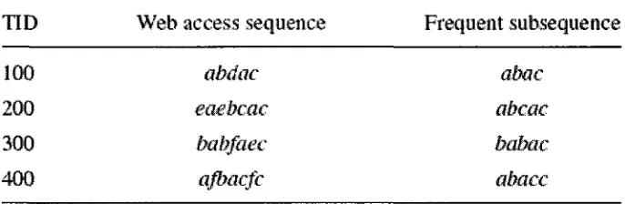
for the WAP tree. Table 26 and Figure 2 represent these 2 stages

TID Web access sequence Frequent subsequence

100

200

300

400

abdac

eaebcac

babfaec

ajbacfc

abac

abcac

babac

abacc

Table 26: The Web Access Sequence Database

Figure 2: The Web Access Pattern tree

The third stage then recursively mines the WAP tree using conditional search. The search

is based on looking for all sequences with common suffix. As the suffix becomes longer,

the remaining search space becomes shorter. The header table created with the WAP tree

above helps construct conditional sequence base for each of the events considered as

suffixes by following the link to all nodes in the WAP tree. This is then used to construct

conditional WAP tree for every suffix considered. The conditional WAP tree is then

recursively mined for frequent events, each time concatenating newly discovered

frequent event with the old ones. The process continues until there are no trees to mine or

Using the above WAP tree as an example, with 75% minimum support, the conditional

WAP tree for suffix sequence 'c' is as shown in Figure 3. This tree is constructed from all

prefix sequences of suffix sequence V . The possible prefix sequences, called conditional

pattern base of suffix sequence V are: aba:2, ab:l, abca:l, ab:-l, baba:l, abac:l, aba:-l.

The negative sequences indicate an overlap in the count because they are already

contained in some other prefixes of 'c'. Because the count of 'c' is less than 75%, it is

removed from the sequence. The resulting sequences are aba:l, aba:l, baba:l, aba:l from

which Figure 3 is constructed. The same process can be used to construct conditional

WAP tree for other suffix sequences, for example 'ac' from Figure 3. The resulting tree is

as shown on Figure 4.

Figure 4: |ac

Figures 3 and 4 show the conditional WAP tree for suffix sequence 'c' and 'ac'

respectively.

The conditional WAP tree 'ac' now confirms that frequent sequences with 'c' as suffix

are ac, aac, bac, abac. The same process can be done with the WAP tree in Figure 2 with

suffixes 'b' and 'a'.

The limitation of this technique is the recursive construction of intermediate WAP tree

2.2.5 PLWAP algorithm

In order to eliminate the need to recursively construct intermediate trees during mining,

PLWAP algorithm was proposed. The approach of Ezeife and Lu (2005) uses position

codes generated for each node such that antecedent/descendant relationships between

nodes can be discovered from the position code. The same WAP tree originally created is

then mined prefix-wise using the position codes as identifiers thereby eliminating

generation of fresh intermediate WAP trees for each sequence mined. The concept of

binary tree is used in generating the position codes. The root has a position code of null.

Starting from the root, all tree nodes are assigned a position code using the following rule.

The position code of the leftmost child node is the position code of its parent

concatenated with ' 1' at the end; the position code of any other node is the same as

appending ' 0 ' to the position code of its closest left sibling.

The algorithm first scans the web access sequence database (WASD) to obtain support

count for all events in it. Events with support greater than or equal to a specified

threshold are said to be frequent. A second scan is then used to eliminate non-frequent

events from the original sequences. These new sequences are then used to construct a

PLWAP-tree with each node representing label, count and position code of the event

along a particular path. The PLWAP-tree is then traversed in a pre-ordered fashion

starting from the root to the left sub-tree followed by the right sub-tree to build to build

the header node linkages. Each event has a queue linking all its nodes in the order in

which they are inserted. The head of each queue is registered in a header table for the

PLWAP tree.

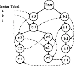
The PLWAP algorithm then recursively mines the PLWAP tree using prefix conditional

TID Web access sequence Frequent subsequence

10G abdac abac

200 eaebcae abcac

300 babfaec bahac

400 ajbacfc abacc

Table 27: The Web Access Database

With the minimum support threshold of 75%, the sequence is reduced to that shown on

the frequent sub sequences column shown above since events 'e' and 'f ' are both 50%

frequent. Events 'e' and 'f ' are not frequent, they are therefore removed in the frequent

subsequences. The resulting reduced sequences are then used to build the PLWAP tree as

shown in Figure 5.

Reader _

Figure 5: The PLWAP tree with the header linkages.

The mining starts by mining sequences with the same prefix. Starting from frequent

1-sequence, the PLWAP algorithm mines starting from the root (for the first time). Using

the header linkage, it traverses the tree to identify frequent 1-sequences by searching for

the first occurrence of an event say 'a'. The position code then helps in preventing

duplicate count of support of an event in the same suffix sub tree. The addition of these