Interactive Thresholding in the Topology Optimization Process

18th International Conference on Structural Mechanics in Reactor Technology (SMiRT 18) Beijing, China, August 7-12, 2005 SMiRT18-F06-4

INTERACTIVE THRESHOLDING IN THE TOPOLOGY OPTIMIZATION

PROCESS

Ryszard Kutylowski

Wroclaw University of Technology,

Institute of Civil Engineering, I-14,

Wyb. Wyspianskiego 27

50-370 Wroclaw, Poland

Phone, Fax: (+48 71) 328 18 89,

E-mail: [email protected]

or [email protected]

ABSTRACT

In this paper it is shown how to obtain the optimal topology of the structure using a new method of thresholding, which gives more refined topology if we compare it with the previous used ordinary thresholding. The thresholding is the part of the topology optimization procedure, which let us to cut (to penalize) very low level density in those design points in which the material is not needed. This procedure is able to change the threshold function during the optimization process according to wide spread analysis of the structure for each design step and additionally for each design point of the structure.

The variation formulation of the optimization problem is considered. The objective is defined as the total strain energy, which is an equivalent to the mean compliance of the structure. The objective is minimizing under the constraint put on the mass of the structure, which is equal to the available mass. The problem is illustrated by the finite element method examples, which is a base to the analysis of the various thresholding paths.

Keywords: Topology optimization, interactive thresholding, minimum compliance, FEM.

1. INTRODUCTION

In general, all designed structures should be as optimal ones. In my previous papers (Kutyłowski 1999, and 2003b), presented in SMiRT Transactions my very fast optimization procedure was used. In this paper the improving of the topology optimization procedure is shown. The improving means, it is to obtained the solution (the topology) with less level of the minimum compliance in comparison to the previous solutions. Such stating the problem let us to obtain stronger structure with the same constraints put on the available mass within the same design domain. It is obvious that this “better” topology will be more “refined”. This improving is possible, because the optimization process becomes more “refined”, what is possible because of improving the thresholding procedure.

All presented procedures may be useful for the nuclear power plant design process, too. This approach is dedicated especially for the designers of even very small nuclear equipment designed for the nuclear power plant, but generally it is useful for example for turbine, steam or electric generators, containment and other elements. Especially, the nuclear power plant we should design for various normal and abnormal load and the design procedure should give us the structure which is an optimal every time independently of the exploitation conditions.

energy in those points is very small, what let us to eliminate the material from these design points. The decision of removing material should be very smart and in this paper the process of founding such “smart procedure” is prepared. It is worth to mention, the literature of this problem is very poor and not recognized. The below shortly presented literature review let us to realize in which direction the research was developed.

Proposed earlier in the literature topology optimization procedures consider only the constant value of the thresholding process. As it was mentioned in Abstract the synonym of the thresholding is penalization of the considered quantity. In the literature, both words, penalization and thresholding mean in this case the same.

Even for the fastest topology optimization procedure presented by Guedes and Taylor (1997), the constant threshold value is used. In mentioned paper it was indicated, how important role plays the value called “a threshold or a cut of value of the material property ρ”. Authors said that the optimization process or in other words in this meaning, the design process is “at the user’s discretion” because of the “threshold value for density”. This shows us the way of research, and suggest us to try to recognize the role of the threshold value plays during the thresholding process.

Penalization of very small considered quantity is well known since years. In Bendsoe (1989) where very interesting new approach was formulated, was additionally indicated that removing mass from the domain which is stressed on the very small level let us to obtain optimal mass distribution. In this paper the penalization was connected together with the Young’s modulus updating definition: and discussion

concerning increasing p (C - is the updated value, - is the initial the Young’s modulus

value). Considered problem was mentioned in Zhou and Rozvany (1991) too. In Sigmund and Petersson (1998)

one can find a discussion based on some earlier papers: a) Allaire and Kohn (1993), b) Allaire, Bonnetier, Francfort and Jouve (1997), c) Haber, Bendsøe and Jog (1996), where the following definition of the threshold function was proposed:

p l k j i l k j i

C

C = ₀ ρ

l k j

i ijkl

C₀

( )

x +c

∫

ρ

(

−ρ

)

dx

ρ 1 where c is a parameter which describes the penalization

level. The constant level of the threshold value was used in Petersson and Sigmund (1998), where this

value was equal to 0.01, where dimensionless quantity were used during the optimization process.

It is clearly seen well known researches in the field were interested the thresholding problem but there is no any details in the literature. This is the reason to recognize all the thresholding problem. It is worth to mention that the decision concerning removing material from the design point is made from the strain energy point of view (relatively small strain energy level in the design point means in this point the material is not needed). Of course this strain energy level must be very low if we compare it with the energy of the other design points. During the optimization process the penalized domain is increasing. Generally the density which is proportional to the strain energy tends to one in those designed points where material is needed and tends to zero in those designed points where material is not needed. We do not know how to that very effectively, which means very fast (within small optimization steps) and by such way, which gives us the optimal solution (for the smallest structural total strain energy).

The analysis concerning using the threshold functions during the optimization process was made in Kutyłowski (2000) where, very effective functions were proposed and verified. Based on this analysis, the general hints how to obtain the optimal solution one can find in Kutyłowski (2002). The strain energy point of view is there the criterion of finding the optimal solution. The wide spread investigation concerning among others the threshold function shows us how important is to find the proper threshold function and let us to realize how complicated problem seems to be. Example of using the topology optimization for the smart structure is proposed in Kutyłowski (2001) the topology which changes according to the changing the load position. Very interesting approach deals with the threshold procedure was shown in Kutyłowski (2003a), where very effective algorithm is presented, which let us to obtain the optimal solution within less optimization steps. The system of redistribution of the available mass is here more effective. It introduces the boundary functions which describe the strain density level from which we can add the mass during the optimization process. Finally it is needed to mention that, the topology optimization problem, in general, is shown in new edition of Bendsøe book, this time written by Bendsøe and Sigmund (2003). The investigation shown below are generally within the minimum compliance topology optimization problem shown in this book.

In this paper the smart optimization procedure is prepared. Among others it consist of the most important part, which is the smart threshold procedure. This procedure is able to change the threshold function during the optimization process according to wide spread analysis of the structure for each design step and additionally for each design point of the structure.

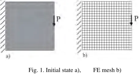
As the numerical example the cantilever beam clamped on its left edge, and loaded by a force P in the middle of its right edge is considered to illustrate how the proposed algorithm in topology optimization procedure works on.

2. THEORETICAL BACKGROUND 2.1 General Theory

The problem is written using variational formulation. The objective is defined as the total strain energy, which is an equivalent to the mean compliance of the structure:

) ( )) ( ( ) ), (

( x C x e e d d m0

F ij kl h

l k j

i _{+ −}

=

_∫

_∫

Ω Ω Ω ρ λ Ω ρ λ

ρ (1)

Some details concerning (1) there are in Kutyłowski (2003b). The elasticity tensor C is a function of Young’s modulus. The constraints put on the mass of the structure are formulate as follow:

l k j i

( ) 1 0

0 = − = m m

H ρj j (2)

In other words the mass of the structure in the j-step of optimization process is equal to the available mass. Because the domain is divided into two parts the mass mj for j-th step is defined as:

v j j

j m m

m

m Ω

Ω _

_ +

= (3)

where Ωm is the domain with material and Ωv is this part of the design domain from which the material was removed (void domain).

After reformulation, the objective for the entire structure finally may be written as:

(

)

(

)

, ) ( ) ) ( ) ( ) ( ) , ), ( ), ( ( _ 0 _ 0 1         − + +         − + + + =

∫

∫

∫

∫

v v m m v m m d x m d x d e e x C d e e x C x x F v v m m v m l k i m l k i m m l k i m l k i v m Ω Ω Ω Ω Ω Ω Ω ε λ Ω ρ λ Ω ε Ω ρ λ λ ε ρ (4)

where ρ is the material density, ε is the relaxed density in empty design points (in those points from which the mass was removed), is the Lagrange multiplier for the domain fulfil by material and is the Lagrange multiplier for those design points from which the mass was removed. is the elasticity tensor for the relaxed material situated in empty design points. If we define the optimal topology obtained for M-th step for i-th

process by we can describe the optimization process as the set of topologies in the form: m λ _λν l k j i C₁ i M γ i M i j γ γ

ε→0

⇒ (5)

where ε tends to zero, which means the density in void domain Ωv tends to zero and the topology becomes optimal.

F_M =minF (6)

The above consideration in formal form usually is called as finding out the stationary point of the objective functional:

(

)

(

)

(

)

(

)

. )

( 0

, )

( 0

, 0 )

( 0

, 0 )

( 0

_ 0

_ 0 1

v v

m m

m d x F

m d x F

e e x C

F

e e x C

F

v v

m m

v m l k i m

l k i

m m l k i m

l k i

Ω Ω

Ω Ω

Ω ε λ

Ω ρ λ

λ ε

ε ε

λ ρ

ρ ρ

∫

∫

= ⇒

= ∂

∂

= ⇒

= ∂

∂

= + ∂

∂ ⇒ = ∂ ∂

= + ∂

∂ ⇒ = ∂ ∂

(7)

The design point may be defined as small part of the design domain as possible (during numerical realization of the problem it may be finite element). During the optimization process the density of each design point is proportional to the strain energy cumulated in this design point. This is the base for FEM algorithm. Important part of this algorithm is the thresholding procedure.

2.2 Thresholding Process

As it was mentioned in Introduction only in one paper it was clear described the kind of used thresholding (Petersson and Sigmund (1998)). It was constant value equal to 0.01. In Kutyłowski (2000) the threshold function was introduced. Using various threshold functions various topologies were obtained for the same structural problem. This means only the analysis from the strain energy point of view gives us an answer concerning the optimal topology of considered problem Kutyłowski (2002). The most important moment of the research was starting to use the threshold function which was a function of the step number j. This let us to increase the value of the threshold function during the optimization process, and let us to cut greater density value for increasing step number. It is obvious that using constant threshold value during the process is not effective. When this value is too small the process sometimes not converges. Sometimes we need even thousand or more steps to obtain optimal topology. When this value is too great sometimes the process not converges, because too great density values were removed from the beginning of the process. It seams, the idea of including the step number to the threshold function definition gave us very good tool for very exact organized optimization process. In this process at the beginning very small density values are removed, next greater and greater are removing and this make the process very slowly and efficiently, in other words it is moderate process.

The thresholding algorithm in finite element notation includes following main steps:

1. removing the mass from the elements which have the strain energy relatively small (the strain energy value is below the threshold function value for considered step number)

2. summing removed mass

3. dividing the mass uniformly into all the elements which the relative density is between 1 and the lower density bound described by ε (relaxed lower bound of the density)

Additionally, the above process let the density to have uniform increase in those design points for which the strain energy is increasing from step to step. The same threshold function was used for the whole process. In this paper we should make an analyze for each step separately to make the decision what kind of cutting is proper for considered step.

j TF

j TF

j TF

α α α

05 . 0

0125 . 0

1 . 0

3 2 1

= = =

(8)

where α is a mass reduction coefficient for available mass m0, which is be defined as: m0 =αm, where

ρ

V

m= . V is the volume of the entire design domain. The above functions are linear. In the below considerations also quadratic functions will be investigated. In the above considerations the Threshold Function sometimes will be described as TF.

The ε quantity was used as follow:

2 2 2

7 1

1 10

j

α ε ε

= = −

(9)

In our consideration important problem is to define in the proper manner the Young’s modulus updating function for each design point separately during every optimization process. For this research following definition is used:

3

0

1( ) 

     =

+ _ρ

ρ

ρ j

j

j E

E (10)

where Ej+1 is a Young’s modulus of each design point separately for j+1 step. is an initial Young’s modulus and is an “artificial” density of each design point for the j step. This definition was widely investigated in Kutyłowski (2002) where it was confirmed the literature intuitions proposed by Bendsøe (1989) and Ramm, Bletzinger, Reitinger and Maute (1994).

0 E

j

ρ

2.3 Thresholding Process Improving

Finding out the optimal topology using a new threshold functions needs the analysis of the strain energy level within each design point separately, which means the base for the analysis is the “map” of the strain energy for the entire structure (entire design domain) for each optimization step. We need these “maps” for the above threshold functions. In the next Chapter 3 it is shown the results of the analysis of increment of the strain energy in each design point.

1 1

− −

− =

j j j

En En En

L (11)

where is the strain energy for considered design point, L is the increment function which is the measurement of the strain energy changing.

1 −

j

En

The strain energy in some design points should increase (for more strengthen design points) and should decrease for these design domains which are becoming voids. If the differences between considered steps are greater in the base solution we may change the threshold function in this direction increasing TF value for the next steps. Every time it is needed to compare all the changes to the base (previous) solution. Especially more complicated TF function (15) was obtained after long analysis of each step comparing it with TF described by (14). The function described by (14) was obtained after the analysis of (13), and so on. Such algorithm needs a lot of time, but it is very effective.

The threshold function analysis deals with the analysis of the mass distribution between two following optimization steps using two various threshold functions. This let to find out the “better” thresholding process.

As it was mentioned in the Introduction as the numerical example the cantilever beam clamped on its left edge, and loaded by a force P in the middle of its right edge is considered. The mass reduction coefficient α is equal to 0.3 in this paper.

Fig. 1. Initial state a), FE mesh b)

The analysis is made for ε described by (9), E described by (10) and for various threshold functions. Functions defined in (8) are the base and we will start from them. Some examples is presented below in separated groups:

1. TF is going from TF2 to TF1.

The first example is made for the beginning function which for each step is increasing additionally about 0.001j for every one step towards to and for

2 TF

1 1

TF ε . Obtained topology is shown in the Fig. 2a. In the Fig.2b and Fig. 2.c topologies for and TF respectively are shown for comparing them with the Fig. 2a. Of course the topology from Fig. 2b was obtained within the smallest step number, but the strain energy (marked in the figures as “en”) is the greatest, which means this topology is the worse one. The below pictures are shown for the step which is just before the 0/1, (black and white) distribution. All the topologies need the postprocessing, but if we compare them it is clear that topology from the Fig. 2a is the best, because of the lowest strain energy level and, because it is the most “refined” topology. The strain energy showed in this picture should be multiplied by 10

1

TF ₂

-3 .

Fig. 2 Topologies for new TF a), for TF₁ b) and for TF₂ c) b) 13th step for

en=2.55

TF₁

a) 62 step, en=2.15 c) 86th step for

en=2.39

TF₂

When we change additionally increasing twice (from 0.001j to 0.002j) the optimal topology we obtain within 57 steps and final strain energy is equal to 2.07 · 10

2 TF

-3

level, smaller than in the Fig. 2.a.

Changing ε intoε2 we can obtain the results written in the Table 1.

Table 1

.

TF Step number for

optimal topology

Strain energy · 10-3

0.0125α j + 0.001j 73 2.04

0.0125α j + 0.002j 61 2.04

0.0125α j 92 2.09

Using (the lowest row in the Table 1.) the result is worse than for the first or the second row for more complicated functions. Increasing the threshold function one can obtain faster the optimal topology (within 61 than 73 steps). Additionally for more softly catching the optimal topology since 58

2 TF

0125

th

step for

j j

TF =0. α +0.002 it was change into TF =0.0125α j+0.001j. The results were the same as in the second row in the Table 1, which means the strain energy and the topologies are the same.

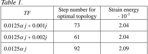
In the Fig. 3 topologies from the Table 1. are shown. They are more “refined” than in the Fig. 2 and the strain energy for them are smaller than for those are shown in the Fig. 2.

a) TF j= 0,0125 α

Fig. 3 Topologies for third a) and second b) row of Table 1. b) = TF j 0,0125 α + 0.002j

2. TF is going from TF1 to TF2.

The second way which was investigated is in opposite to the first one shown above. The question arise: should we at the beginning to cut relatively greater density value? When we should do that more slowly? The following functions were investigated:

2 1

1 1 1

005 . 0

01 . 0

005 . 0

001 . 0

j TF

TF

j TF

TF

j TF

TF

j TF

TF

− =

− =

− =

− =

(12)

Unfortunately solutions were not satisfied for both ε relaxed functions. Solutions were similar to those obtained for TF1. Additionally it was not impossible to obtain solution for the last function of (12).

3. TF is going from TF1 using various functions.

3.1 Some functions were analysed. Let me start with the functions defined as follow: for the first 5 steps there is . Aftermaking the general distribution it is needed to make the process more slowly and this is why the function is changing into the following form:

1 TF

15 . 0 5

6

2 1

+ = >

= <

TF TF j

for

TF TF j

for

The constant value 0.15 is the value of the TF1 for 5 th

step. In the Table 2. the results are shown:

Table 2.

ε Step number for optimal topology

Strain energy · 10-3

1

ε 59 2.17

2

ε 52 2.08

The results are better than obtained in the Fig. 2.c. for ε1 (obtained within 59 steps with energy equal to

2.17, instead within 86 steps with energy 2.39) and in the Table 1. (last row) for ε2(obtained within 52 steps

with energy equal to 2.08, instead within 92 steps with energy 2.09).

3.2 Next the TF is changing into the following form:

j TF

TF j

for

TF TF j

for

002 . 0 15 . 0 5

6

2 1

+ + = >

= <

(14)

For ε2 the optimal topology for this TF is obtained within only 36 steps smaller than in the Table 2. in the

second row (within 52 steps), but the strain energy is equal to 2.12· 10-3, what is greater value than it is in the Table 2. Similar solution is for ε1. Generally considered solution does not improve the strain energy.

Table 3.

ε Step number for optimal topology

Strain energy · 10-3

1

ε 34 2.97

2

ε 36 2.12

The formula (14) was changed by this way next: 0.15 was changed into 0.1. Unfortunately for both ε it is no possible to obtain optimal topology better than it is shown in the Table 3, but the analysis of obtained topologies for the step numbers since 6 into 22 gives the information the process is going a little bit better than for (14). This is why this modified equation (14) is the base for the below investigations. Details concerning these solutions there are in the Table 4. Solution for ε1is obtained for the topology with the shades of grey, which

means this topology for minimum strain energy for this process needs the postprocessing.

Table 4.

ε Step number for optimal topology

Strain energy · 10-3

1

ε 32 2.51

2

ε 43 2.21

3.3 The analysis concerning the problem when to speed thresholding process and when to make it more slowly gives us an answer, that for the first steps stronger thresholding it is better how it was defined in (14). Middle part of the modified threshold function should cut slowly the mass from those design points for which the mass is not needed. Finally when we are closer to the optimal topology the thresholding process should be faster. To find the proper moment for increasing the threshold function is not easy and it depends on the history of topologies of considered process and depends on used the TF formulas. Let us consider the problem for

1

ε

044 . 0 001 . 0 1 . 0 21 002 . 0 1 . 0 22 5 6 2 2 1 + + + = > + + = < > = < j TF TF j for j TF TF j for and j for TF TF j for (15)

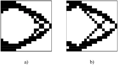
which gives us the optimal topology within 43 steps with the lowest level of the strain energy (1.98· 10-3). This is the best results obtained during this investigation, shown in the Fig. 4a. The same TF function used for ε=ε2

let us to obtain the optimal topology within 49 steps but the strain energy is very similar, it is equal to 1.99· 10-3 (Fig. 4b). Unfortunately for this case (for ε=ε2) the algorithm converges slower and must to overcome the

problem of leaving very small density in two regions situated in white right up and right down corners (Fig. 5 for 30th step).

a)

Fig. 4 Topologies for ε1 a) and for ε2 b) b)

The details results are shown in the Table 5.

Table 5.

ε TF Step number for

optimal topology

Strain energy · 10-3

1 ε 044 . 0 001 . 0 1 . 0 21 002 . 0 1 . 0 22 5 6 2 2 1 + + + = > + + = < > = < j TF TF j for j TF TF j for and j for TF TF j for 43 1.98 2

ε The same as above 49 1.99

The topologies for some steps (30th, 40th and 41st) for ε=ε2 are shown in number mode in the Fig. 5.

30th step 40th step 41st step

Fig. 5 Topologies for (15) and 2ε

1.0 1.0 1.0 1.0 1.0 0.8 0.6 0.0 0.0 0.0 0.6 0.9 1.0 1.0 1.0 1.0 1.0 0.7 0.0 0.0 0.9 0.9 0.9 0.7 0.6 0.8 1.0 1.0 1.0 0.7 0.0 0.0 1.0 0.8 0.6 0.6 0.8 1.0 1.0 1.0 0.8 0.6 0.0 0.0

0.6 0.6 0.7 1.0 1.0 1.0 0.8 0.6 0.0 0.6 0.5 0.6 0.9 1.0 1.0 0.8

0.6 0.6 0.6 0.9 1.0 1.0 0.6 0.6 0.6 1.0 1.0 0.6 0.6 0.6 0.6 0.6 0.7 1.0 0.6

0.6 0.6 0.6 0.6 0.6 0.6 1.0 0.6 0.6 0.6 0.6 0.6 0.6 1.0 0.6 0.6 0.6 0.6 0.6 0.7 1.0 0.6 0.6 0.6 0.6 1.0 1.0 0.6 0.6 0.6 0.9 1.0 1.0 0.6 0.5 0.6 0.9 1.0 1.0 0.8 0.6 0.6 0.7 1.0 1.0 1.0 0.8 0.6 0.0 1.0 0.8 0.6 0.6 0.8 1.0 1.0 1.0 0.8 0.6 0.0 0.0 0.9 0.9 0.9 0.7 0.6 0.8 1.0 1.0 1.0 0.7 0.0 0.0 0.6 0.9 1.0 1.0 1.0 1.0 1.0 0.7 0.0 0.0 1.0 1.0 1.0 1.0 1.0 0.8 0.6 0.0 0.0 0.0

1.0 1.0 1.0 1.0 1.0 1.0 1.0 1.0 1.0 1.0 1.0 1.0 0.9 1.0 1.0 1.0 0.9 0.8 1.0 1.0 1.0 1.0 0.9 1.0 1.0 0.8 0.8 1.0 1.0 1.0 1.0 0.9

0.8 0.8 0.9 1.0 1.0 1.0 1.0 0.9 0.8 1.0 1.0 1.0 1.0

0.9 0.8 1.0 1.0 1.0 0.8 0.9 1.0 1.0

0.8 0.9 0.9 1.0 0.8 0.9 0.8 0.8 1.0 0.8 0.9 0.8 0.8 1.0 0.8 0.9 0.9 1.0 0.8 0.9 1.0 1.0 0.9 0.8 1.0 1.0 1.0 0.9 0.8 1.0 1.0 1.0 1.0 0.8 0.8 0.9 1.0 1.0 1.0 1.0 1.0 1.0 0.8 0.8 1.0 1.0 1.0 1.0 0.9 1.0 1.0 1.0 0.9 0.8 1.0 1.0 1.0 1.0 0.9

1.0 1.0 1.0 1.0 1.0 1.0 0.9 1.0 1.0 1.0 1.0 1.0 1.0

1.0 1.0 1.0 1.0 1.0 1.0 1.0 1.0 1.0 1.0 1.0 1.0 0.9 1.0 1.0 1.0 0.9 0.9 1.0 1.0 1.0 1.0 0.9 1.0 1.0 0.8 0.9 1.0 1.0 1.0 1.0 1.0

0.8 0.8 0.9 1.0 1.0 1.0 1.0 0.9 0.9 1.0 1.0 1.0 1.0

0.9 0.8 1.0 1.0 1.0 0.9 0.9 1.0 1.0

0.9 0.9 0.9 1.0 0.9 0.9 0.8 1.0 0.9 0.9 0.8 1.0 0.9 0.9 0.9 1.0 0.9 0.9 1.0 1.0 0.9 0.8 1.0 1.0 1.0 0.9 0.9 1.0 1.0 1.0 1.0 0.8 0.8 0.9 1.0 1.0 1.0 1.0 1.0 1.0 0.8 0.9 1.0 1.0 1.0 1.0 1.0 1.0 1.0 1.0 0.9 0.9 1.0 1.0 1.0 1.0 0.9

In the Fig. 5 we can see the direction of moving mass especially for some steps just before the optimal topology (for 40th and for 41st step). For 42nd step there is very small number of the elements with the density very close to 1. Step number 43 is presented in the black and white mode in the Fig. 4 b.

When we change in the formula (15) the step number from 21 to 29 (third row in (14)) the solutions for both ε do not converge. This shows how “weak line we are going on” and how difficult is to define the proper topology process parameters to find out the optimal topology.

For comparing the optimization process which is going on using previous thresholding path and the new one the next figures were prepared. For both pictures the ε=ε1. In the Fig. 6 some steps for are shown. We

can see not refined topology obtained within very small steps number (within 14 steps black and white topology). The strain energy is equal to 2.55 · 10

1 TF

-3

and this topology is very difficult to call the optimal topology.

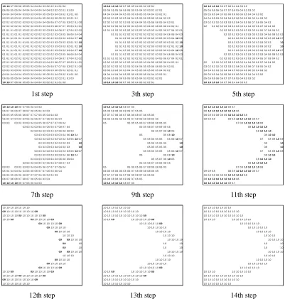
In the next figure (Fig. 7) the optimization process for the threshold function defined in the equation (15) is presented. It shows how the improved procedure works. The topologies for 5th steps are the same (in the Fig. 6 and in the Fig. 7). The process was finished for the 14th step in the Fig. 6, but in the Fig. 7 for the 15th step we have the topology with the wide spectrum of densities (since 0.2 to 1.0). This means making the process slower between

1.0 1.00.7 0.6 0.6 0.5 0.5 0.4 0.4 0.4 0.3 0.2 0.2 0.1 0.1 0.0 0.6 0.6 0.5 0.5 0.4 0.4 0.4 0.4 0.4 0.4 0.4 0.4 0.3 0.2 0.2 0.1 0.1 0.0 0.4 0.4 0.4 0.4 0.4 0.3 0.3 0.3 0.4 0.4 0.5 0.5 0.5 0.4 0.3 0.2 0.1 0.1 0.0 0.3 0.3 0.3 0.3 0.3 0.3 0.3 0.3 0.4 0.4 0.5 0.6 0.6 0.6 0.5 0.3 0.2 0.1 0.1 0.2 0.2 0.2 0.2 0.2 0.2 0.3 0.3 0.3 0.4 0.4 0.5 0.6 0.7 0.7 0.5 0.3 0.2 0.1 0.0 0.2 0.2 0.2 0.2 0.2 0.2 0.2 0.2 0.3 0.3 0.3 0.4 0.5 0.6 0.7 0.7 0.5 0.3 0.1 0.1 0.1 0.1 0.1 0.2 0.2 0.2 0.2 0.2 0.2 0.2 0.2 0.3 0.3 0.4 0.6 0.7 0.7 0.4 0.2 0.2 0.1 0.1 0.1 0.1 0.1 0.2 0.2 0.2 0.2 0.2 0.2 0.2 0.2 0.3 0.3 0.5 0.6 0.6 0.4 0.4 0.1 0.1 0.1 0.1 0.1 0.1 0.2 0.2 0.2 0.2 0.2 0.2 0.2 0.3 0.3 0.3 0.3 0.4 0.71.0 0.1 0.1 0.1 0.1 0.1 0.1 0.1 0.2 0.2 0.2 0.2 0.2 0.3 0.3 0.3 0.3 0.2 0.1 0.21.0 0.1 0.1 0.1 0.1 0.1 0.1 0.1 0.2 0.2 0.2 0.2 0.2 0.3 0.3 0.3 0.3 0.2 0.1 0.21.0 0.1 0.1 0.1 0.1 0.1 0.1 0.2 0.2 0.2 0.2 0.2 0.2 0.2 0.3 0.3 0.3 0.3 0.4 0.71.0 0.1 0.1 0.1 0.1 0.1 0.2 0.2 0.2 0.2 0.2 0.2 0.2 0.2 0.3 0.3 0.5 0.6 0.6 0.4 0.4 0.1 0.1 0.1 0.2 0.2 0.2 0.2 0.2 0.2 0.2 0.2 0.3 0.3 0.4 0.6 0.7 0.7 0.4 0.2 0.2 0.2 0.2 0.2 0.2 0.2 0.2 0.2 0.2 0.3 0.3 0.3 0.4 0.5 0.6 0.7 0.7 0.5 0.3 0.1 0.1 0.2 0.2 0.2 0.2 0.2 0.2 0.3 0.3 0.3 0.4 0.4 0.5 0.6 0.7 0.7 0.5 0.3 0.2 0.1 0.0 0.3 0.3 0.3 0.3 0.3 0.3 0.3 0.3 0.4 0.4 0.5 0.6 0.6 0.6 0.5 0.3 0.2 0.1 0.1 0.4 0.4 0.4 0.4 0.4 0.3 0.3 0.3 0.4 0.4 0.5 0.5 0.5 0.4 0.3 0.2 0.1 0.1 0.0 0.6 0.6 0.5 0.5 0.4 0.4 0.4 0.4 0.4 0.4 0.4 0.4 0.3 0.2 0.2 0.1 0.1 0.0 1.0 1.00.7 0.6 0.6 0.5 0.5 0.4 0.4 0.4 0.3 0.2 0.2 0.1 0.1 0.0

1.0 1.0 1.0 1.00.8 0.7 0.6 0.5 0.4 0.3 0.2 0.2 0.1 0.5 0.6 0.5 0.5 0.6 0.6 0.6 0.5 0.5 0.4 0.3 0.3 0.2 0.2 0.1 0.4 0.4 0.4 0.4 0.4 0.5 0.5 0.5 0.6 0.5 0.5 0.4 0.4 0.3 0.2 0.1 0.3 0.3 0.3 0.3 0.3 0.3 0.4 0.4 0.5 0.5 0.6 0.5 0.5 0.5 0.4 0.3 0.2 0.2 0.2 0.2 0.2 0.2 0.3 0.3 0.3 0.4 0.4 0.5 0.5 0.6 0.6 0.5 0.4 0.3 0.1 0.2 0.2 0.2 0.2 0.2 0.2 0.2 0.3 0.3 0.3 0.3 0.4 0.5 0.6 0.6 0.6 0.4 0.2 0.1 0.1 0.1 0.1 0.2 0.2 0.2 0.2 0.2 0.2 0.2 0.3 0.3 0.3 0.4 0.5 0.6 0.7 0.4 0.2 0.1

0.1 0.1 0.1 0.2 0.2 0.2 0.2 0.2 0.2 0.2 0.2 0.3 0.3 0.4 0.6 0.8 0.4 0.3 0.1 0.1 0.2 0.2 0.2 0.2 0.2 0.2 0.2 0.3 0.3 0.3 0.3 0.3 0.41.00.8 0.1 0.1 0.1 0.2 0.2 0.2 0.2 0.2 0.2 0.3 0.3 0.3 0.3 0.2 0.1 0.21.0 0.1 0.1 0.1 0.2 0.2 0.2 0.2 0.2 0.2 0.3 0.3 0.3 0.3 0.2 0.1 0.21.0 0.1 0.1 0.2 0.2 0.2 0.2 0.2 0.2 0.2 0.3 0.3 0.3 0.3 0.3 0.41.00.8 0.1 0.1 0.1 0.2 0.2 0.2 0.2 0.2 0.2 0.2 0.2 0.3 0.3 0.4 0.6 0.8 0.4 0.3 0.1 0.1 0.1 0.2 0.2 0.2 0.2 0.2 0.2 0.2 0.3 0.3 0.3 0.4 0.5 0.6 0.7 0.4 0.2 0.1 0.2 0.2 0.2 0.2 0.2 0.2 0.2 0.3 0.3 0.3 0.3 0.4 0.5 0.6 0.6 0.6 0.4 0.2 0.1 0.2 0.2 0.2 0.2 0.2 0.3 0.3 0.3 0.4 0.4 0.5 0.5 0.6 0.6 0.5 0.4 0.3 0.1 0.3 0.3 0.3 0.3 0.3 0.3 0.4 0.4 0.5 0.5 0.6 0.5 0.5 0.5 0.4 0.3 0.2 0.4 0.4 0.4 0.4 0.4 0.5 0.5 0.5 0.6 0.5 0.5 0.4 0.4 0.3 0.2 0.1 0.5 0.6 0.5 0.5 0.6 0.6 0.6 0.5 0.5 0.4 0.3 0.3 0.2 0.2 0.1 1.0 1.0 1.0 1.00.8 0.7 0.6 0.5 0.4 0.3 0.2 0.2 0.1

1.0 1.0 1.0 1.00.9 0.7 0.6 0.4 0.4 0.3 0.2 0.5 0.6 0.6 0.6 0.6 0.7 0.7 0.6 0.5 0.4 0.3 0.3 0.2 0.5 0.5 0.5 0.4 0.5 0.5 0.6 0.6 0.6 0.6 0.5 0.4 0.4 0.3 0.2 0.4 0.4 0.3 0.3 0.3 0.4 0.4 0.5 0.6 0.6 0.6 0.6 0.5 0.4 0.3 0.2 0.3 0.2 0.2 0.2 0.3 0.3 0.3 0.3 0.4 0.5 0.5 0.6 0.7 0.6 0.5 0.4 0.2 0.2 0.2 0.2 0.2 0.2 0.3 0.3 0.3 0.3 0.4 0.4 0.5 0.6 0.7 0.6 0.4 0.2

0.2 0.2 0.2 0.2 0.3 0.3 0.3 0.3 0.3 0.4 0.5 0.7 0.8 0.4 0.2 0.2 0.2 0.2 0.3 0.3 0.3 0.3 0.3 0.3 0.3 0.4 0.6 0.9 0.3 0.3

0.2 0.2 0.2 0.3 0.3 0.3 0.3 0.3 0.3 0.3 0.3 0.51.00.7 0.2 0.2 0.2 0.3 0.3 0.3 0.3 0.3 0.3 0.3 0.2 1.0 0.2 0.2 0.2 0.3 0.3 0.3 0.3 0.3 0.3 0.3 0.2 1.0 0.2 0.2 0.2 0.3 0.3 0.3 0.3 0.3 0.3 0.3 0.3 0.51.00.7 0.2 0.2 0.2 0.3 0.3 0.3 0.3 0.3 0.3 0.3 0.4 0.6 0.9 0.3 0.3 0.2 0.2 0.2 0.2 0.3 0.3 0.3 0.3 0.3 0.4 0.5 0.7 0.8 0.4 0.2 0.2 0.2 0.2 0.2 0.2 0.3 0.3 0.3 0.3 0.4 0.4 0.5 0.6 0.7 0.6 0.4 0.2 0.3 0.2 0.2 0.2 0.3 0.3 0.3 0.3 0.4 0.5 0.5 0.6 0.7 0.6 0.5 0.4 0.2 0.4 0.4 0.3 0.3 0.3 0.4 0.4 0.5 0.6 0.6 0.6 0.6 0.5 0.4 0.3 0.2 0.5 0.5 0.5 0.4 0.5 0.5 0.6 0.6 0.6 0.6 0.5 0.4 0.4 0.3 0.2 0.5 0.6 0.6 0.6 0.6 0.7 0.7 0.6 0.5 0.4 0.3 0.3 0.2 1.0 1.0 1.0 1.00.9 0.7 0.6 0.4 0.4 0.3 0.2

1.0 1.0 1.0 1.00.9 0.7 0.6 0.5 0.4 0.3 0.6 0.7 0.6 0.6 0.7 0.8 0.7 0.6 0.5 0.4 0.3 0.3 0.6 0.5 0.5 0.5 0.5 0.6 0.7 0.7 0.7 0.6 0.5 0.4 0.4 0.3 0.5 0.4 0.4 0.4 0.4 0.4 0.5 0.5 0.6 0.7 0.7 0.6 0.6 0.5 0.4 0.3 0.3 0.3 0.3 0.3 0.3 0.4 0.4 0.5 0.6 0.7 0.7 0.7 0.6 0.4

0.3 0.3 0.3 0.3 0.4 0.4 0.5 0.6 0.7 0.8 0.7 0.4 0.3 0.3 0.3 0.3 0.3 0.4 0.4 0.6 0.8 0.9 0.4

0.3 0.3 0.3 0.3 0.3 0.3 0.3 0.4 0.61.00.4 0.3 0.3 0.3 0.3 0.3 0.3 0.3 0.3 0.3 0.51.00.7

0.3 0.3 0.3 0.3 0.4 0.4 0.3 0.3 1.0 0.3 0.3 0.3 0.3 0.4 0.4 0.3 0.3 1.0 0.3 0.3 0.3 0.3 0.3 0.3 0.3 0.3 0.3 0.51.00.7 0.3 0.3 0.3 0.3 0.3 0.3 0.3 0.4 0.61.00.4 0.3 0.3 0.3 0.3 0.3 0.4 0.4 0.6 0.8 0.9 0.4 0.3 0.3 0.3 0.3 0.4 0.4 0.5 0.6 0.7 0.8 0.7 0.4 0.3 0.3 0.3 0.3 0.3 0.3 0.4 0.4 0.5 0.6 0.7 0.7 0.7 0.6 0.4 0.5 0.4 0.4 0.4 0.4 0.4 0.5 0.5 0.6 0.7 0.7 0.6 0.6 0.5 0.4 0.6 0.5 0.5 0.5 0.5 0.6 0.7 0.7 0.7 0.6 0.5 0.4 0.4 0.3 0.6 0.7 0.6 0.6 0.7 0.8 0.7 0.6 0.5 0.4 0.3 0.3 1.0 1.0 1.0 1.00.9 0.7 0.6 0.5 0.4 0.3

1.0 1.0 1.0 1.0 1.00.8 0.7 0.5 0.6 0.8 0.8 0.8 0.9 0.9 0.9 0.7 0.6 0.5 0.7 0.7 0.7 0.6 0.6 0.7 0.8 0.9 0.8 0.7 0.6 0.5 0.5 0.6 0.6 0.5 0.5 0.5 0.5 0.6 0.7 0.8 0.9 0.8 0.8 0.6 0.5 0.5 0.5 0.5 0.5 0.6 0.7 0.8 0.9 0.8 0.6 0.5

0.5 0.5 0.6 0.7 0.9 0.9 0.8 0.5 0.5 0.5 0.7 0.91.00.5 0.5 0.5 0.81.0

0.5 0.5 0.5 0.5 0.5 0.5 0.61.00.7 0.5 0.5 0.5 0.5 0.5 1.0 0.5 0.5 0.5 0.5 0.5 1.0 0.5 0.5 0.5 0.5 0.5 0.5 0.61.00.7 0.5 0.5 0.81.0

0.5 0.5 0.7 0.91.00.5 0.5 0.5 0.6 0.7 0.9 0.9 0.8 0.5 0.5 0.5 0.5 0.5 0.6 0.7 0.8 0.9 0.8 0.6 0.5 0.6 0.6 0.5 0.5 0.5 0.5 0.6 0.7 0.8 0.9 0.8 0.8 0.6 0.5 0.7 0.7 0.7 0.6 0.6 0.7 0.8 0.9 0.8 0.7 0.6 0.5 0.5 0.6 0.8 0.8 0.8 0.9 0.9 0.9 0.7 0.6 0.5 1.0 1.0 1.0 1.0 1.00.8 0.7 0.5

1.0 1.0 1.0 1.0 1.0 1.00.9 0.7 0.81.0 1.0 1.0 1.0 1.0 1.0 1.00.8 0.9 0.9 0.9 0.8 0.8 0.91.0 1.0 1.0 1.00.8 0.9 0.9 0.8 0.8 0.91.0 1.0 1.0 1.00.8 0.7

0.7 0.81.0 1.0 1.0 1.00.8 0.81.0 1.0 1.0 1.0

0.81.0 1.0 1.0 0.91.0 1.0 0.7 0.8 0.91.00.9

0.8 1.0 0.8 1.0 0.7 0.8 0.91.00.9

0.91.0 1.0 0.81.0 1.0 1.0 0.81.0 1.0 1.0 1.0 0.7 0.81.0 1.0 1.0 1.00.8 0.9 0.9 0.8 0.8 0.91.0 1.0 1.0 1.00.8 0.7 0.9 0.9 0.9 0.8 0.8 0.91.0 1.0 1.0 1.00.8 0.81.0 1.0 1.0 1.0 1.0 1.0 1.00.8 1.0 1.0 1.0 1.0 1.0 1.00.9 0.7

1.0 1.0 1.0 1.0 1.0 1.0 1.0 1.0 1.0 1.0 1.0 1.0 1.0 1.0 1.0 1.0 1.0 1.0 1.0 1.0 1.0 1.0 1.0 1.0 1.0 1.00.9 1.0 1.00.9 1.0 1.0 1.0 1.0 1.00.9

1.0 1.0 1.0 1.0 1.00.9 1.0 1.0 1.0 1.0 1.0

1.0 1.0 1.0 1.0 1.0 1.0 1.0

1.0 1.0 1.0 1.0 1.0 1.0 1.0 1.0 1.0 1.0 1.0 1.0 1.0 1.0 1.0 1.0 1.0 1.0 1.0 1.0 1.0 1.0 1.0 1.0 1.0 1.0 1.0 1.0 1.00.9 1.0 1.00.9 1.0 1.0 1.0 1.0 1.00.9 1.0 1.0 1.0 1.0 1.0 1.0 1.0 1.0 1.0 1.00.9 1.0 1.0 1.0 1.0 1.0 1.0 1.0 1.0 1.0 1.0 1.0 1.0 1.0 1.0 1.0 1.0

1.0 1.0 1.0 1.0 1.0 1.0 1.0 1.0 1.0 1.0 1.0 1.0 1.0 1.0 1.0 1.0 1.0 1.0 1.0 1.0 1.0 1.0 1.0 1.0 1.0 1.0 1.0 1.0 1.0 1.0 1.0 1.0 1.0 1.0

1.0 1.0 1.0 1.0 1.0 1.0 1.0 1.0 1.0 1.0

1.0 1.0 1.0 1.0 1.0 1.0 1.0

1.0 1.0 1.0 1.0 1.0 1.0 1.0 1.0 1.0 1.0 1.0 1.0 1.0 1.0 1.0 1.0 1.0 1.0 1.0 1.0 1.0 1.0 1.0 1.0 1.0 1.0 1.0 1.0 1.0 1.0 1.0 1.0 1.0 1.0 1.0 1.0 1.0 1.0 1.0 1.0 1.0 1.0 1.0 1.0 1.0 1.0 1.0 1.0 1.0 1.0 1.0 1.0 1.0 1.0 1.0 1.0 1.0 1.0 1.0 1.0 1.0 1.0 1.0 1.0 1.0 1.0 1.0 1.0 1.0 1.0

0.91.0 1.0 1.0 1.0 1.0 1.0 1.00.9 1.0 1.0 1.0 1.00.91.0 1.0 1.0 1.0 1.00.9 1.0 1.00.9 0.91.0 1.0 1.0 1.00.9

0.91.0 1.0 1.0 1.00.9 0.91.0 1.0 1.0 1.0

0.91.0 1.0 1.0 1.0 1.0 1.0 0.9 0.91.0 1.0 1.0

0.9 1.0 0.9 1.0 0.9 0.91.0 1.0 1.0

1.0 1.0 1.0 0.91.0 1.0 1.0 0.91.0 1.0 1.0 1.0 0.91.0 1.0 1.0 1.00.9 1.0 1.00.9 0.91.0 1.0 1.0 1.00.9 1.0 1.0 1.0 1.00.91.0 1.0 1.0 1.0 1.00.9 0.91.0 1.0 1.0 1.0 1.0 1.0 1.00.9 1.0 1.0 1.0 1.0 1.0 1.0 1.0

1st step 3th step 5th step

9th step 11th step

7th step

12th step 13th step 14th step

the step numbers 6 and 22 we obtained possibility to obtain more refined topology with the smaller level of the strain energy. For the step numbers 30 and 38 we can observe how the mass have moved (in which direction it was moved) faster than it was between the step numbers 6 and 22. Since 38th step only improving and coming up to density value equal to 1 we can see. Very similar the process is going on for the topology shown in the Fig. 5 and Fig. 4 b obtained for the threshold function defined in (15) for ε=ε2. Since the 30

th

step number shown in the

Fig. 5 into the 43rd step number there is the process of final refinement of the topology which was have arisen during the slower thresholding process (between the step numbers 6 and 22).

Fig. 7 Topologies for (15) and 1ε

1.0 1.0 0.7 0.6 0.6 0.5 0.5 0.4 0.4 0.4 0.3 0.2 0.2 0.1 0.1 0.0 0.6 0.6 0.5 0.5 0.4 0.4 0.4 0.4 0.4 0.4 0.4 0.4 0.3 0.2 0.2 0.1 0.1 0.0 0.4 0.4 0.4 0.4 0.4 0.3 0.3 0.3 0.4 0.4 0.5 0.5 0.5 0.4 0.3 0.2 0.1 0.1 0.0 0.3 0.3 0.3 0.3 0.3 0.3 0.3 0.3 0.4 0.4 0.5 0.6 0.6 0.6 0.5 0.3 0.2 0.1 0.1 0.2 0.2 0.2 0.2 0.2 0.2 0.3 0.3 0.3 0.4 0.4 0.5 0.6 0.7 0.7 0.5 0.3 0.2 0.1 0.0 0.2 0.2 0.2 0.2 0.2 0.2 0.2 0.2 0.3 0.3 0.3 0.4 0.5 0.6 0.7 0.7 0.5 0.3 0.1 0.1 0.1 0.1 0.1 0.2 0.2 0.2 0.2 0.2 0.2 0.2 0.2 0.3 0.3 0.4 0.6 0.7 0.7 0.4 0.2 0.2 0.1 0.1 0.1 0.1 0.1 0.2 0.2 0.2 0.2 0.2 0.2 0.2 0.2 0.3 0.3 0.5 0.6 0.6 0.4 0.4 0.1 0.1 0.1 0.1 0.1 0.1 0.2 0.2 0.2 0.2 0.2 0.2 0.2 0.3 0.3 0.3 0.3 0.4 0.7 1.0 0.1 0.1 0.1 0.1 0.1 0.1 0.1 0.2 0.2 0.2 0.2 0.2 0.3 0.3 0.3 0.3 0.2 0.1 0.2 1.0 0.1 0.1 0.1 0.1 0.1 0.1 0.1 0.2 0.2 0.2 0.2 0.2 0.3 0.3 0.3 0.3 0.2 0.1 0.2 1.0 0.1 0.1 0.1 0.1 0.1 0.1 0.2 0.2 0.2 0.2 0.2 0.2 0.2 0.3 0.3 0.3 0.3 0.4 0.7 1.0 0.1 0.1 0.1 0.1 0.1 0.2 0.2 0.2 0.2 0.2 0.2 0.2 0.2 0.3 0.3 0.5 0.6 0.6 0.4 0.4 0.1 0.1 0.1 0.2 0.2 0.2 0.2 0.2 0.2 0.2 0.2 0.3 0.3 0.4 0.6 0.7 0.7 0.4 0.2 0.2 0.2 0.2 0.2 0.2 0.2 0.2 0.2 0.2 0.3 0.3 0.3 0.4 0.5 0.6 0.7 0.7 0.5 0.3 0.1 0.1 0.2 0.2 0.2 0.2 0.2 0.2 0.3 0.3 0.3 0.4 0.4 0.5 0.6 0.7 0.7 0.5 0.3 0.2 0.1 0.0 0.3 0.3 0.3 0.3 0.3 0.3 0.3 0.3 0.4 0.4 0.5 0.6 0.6 0.6 0.5 0.3 0.2 0.1 0.1 0.4 0.4 0.4 0.4 0.4 0.3 0.3 0.3 0.4 0.4 0.5 0.5 0.5 0.4 0.3 0.2 0.1 0.1 0.0 0.6 0.6 0.5 0.5 0.4 0.4 0.4 0.4 0.4 0.4 0.4 0.4 0.3 0.2 0.2 0.1 0.1 0.0 1.0 1.0 0.7 0.6 0.6 0.5 0.5 0.4 0.4 0.4 0.3 0.2 0.2 0.1 0.1 0.0

1.0 1.0 1.0 1.0 0.9 0.7 0.6 0.4 0.4 0.3 0.2 0.5 0.6 0.6 0.6 0.6 0.7 0.7 0.6 0.5 0.4 0.3 0.3 0.2 0.5 0.5 0.5 0.4 0.5 0.5 0.6 0.6 0.6 0.6 0.5 0.4 0.4 0.3 0.2 0.4 0.4 0.3 0.3 0.3 0.4 0.4 0.5 0.6 0.6 0.6 0.6 0.5 0.4 0.3 0.2 0.3 0.2 0.2 0.2 0.3 0.3 0.3 0.3 0.4 0.5 0.5 0.6 0.7 0.6 0.5 0.4 0.2 0.2 0.2 0.2 0.2 0.2 0.3 0.3 0.3 0.3 0.4 0.4 0.5 0.6 0.7 0.6 0.4 0.2

0.2 0.2 0.2 0.2 0.3 0.3 0.3 0.3 0.3 0.4 0.5 0.7 0.8 0.4 0.2 0.2 0.2 0.2 0.3 0.3 0.3 0.3 0.3 0.3 0.3 0.4 0.6 0.9 0.3 0.3

0.2 0.2 0.2 0.3 0.3 0.3 0.3 0.3 0.3 0.3 0.3 0.5 1.0 0.7 0.2 0.2 0.2 0.3 0.3 0.3 0.3 0.3 0.3 0.3 0.2 1.0 0.2 0.2 0.2 0.3 0.3 0.3 0.3 0.3 0.3 0.3 0.2 1.0 0.2 0.2 0.2 0.3 0.3 0.3 0.3 0.3 0.3 0.3 0.3 0.5 1.0 0.7 0.2 0.2 0.2 0.3 0.3 0.3 0.3 0.3 0.3 0.3 0.4 0.6 0.9 0.3 0.3 0.2 0.2 0.2 0.2 0.3 0.3 0.3 0.3 0.3 0.4 0.5 0.7 0.8 0.4 0.2 0.2 0.2 0.2 0.2 0.2 0.3 0.3 0.3 0.3 0.4 0.4 0.5 0.6 0.7 0.6 0.4 0.2 0.3 0.2 0.2 0.2 0.3 0.3 0.3 0.3 0.4 0.5 0.5 0.6 0.7 0.6 0.5 0.4 0.2 0.4 0.4 0.3 0.3 0.3 0.4 0.4 0.5 0.6 0.6 0.6 0.6 0.5 0.4 0.3 0.2 0.5 0.5 0.5 0.4 0.5 0.5 0.6 0.6 0.6 0.6 0.5 0.4 0.4 0.3 0.2 0.5 0.6 0.6 0.6 0.6 0.7 0.7 0.6 0.5 0.4 0.3 0.3 0.2 1.0 1.0 1.0 1.0 0.9 0.7 0.6 0.4 0.4 0.3 0.2

1st step

1.0 1.0 1.0 1.0 0.9 0.6 0.5 0.3 0.3 0.4 0.7 0.7 0.7 0.8 0.9 0.8 0.6 0.4 0.3 0.3 0.6 0.6 0.5 0.5 0.5 0.6 0.7 0.8 0.8 0.6 0.4 0.3 0.3 0.5 0.4 0.4 0.3 0.3 0.4 0.4 0.5 0.7 0.8 0.8 0.7 0.5 0.3 0.3 0.3 0.3 0.2 0.3 0.3 0.3 0.3 0.3 0.4 0.5 0.6 0.8 0.8 0.7 0.5 0.3

0.3 0.3 0.3 0.3 0.3 0.3 0.3 0.4 0.6 0.8 0.9 0.7 0.3 0.3 0.3 0.3 0.3 0.3 0.3 0.3 0.3 0.4 0.6 0.9 1.0 0.3

0.3 0.3 0.3 0.3 0.3 0.3 0.3 0.3 0.3 0.4 0.6 1.0 0.3 0.2 0.2 0.3 0.3 0.3 0.3 0.3 0.3 0.3 0.3 0.3 0.4 1.0 0.5

0.2 0.3 0.3 0.3 0.3 0.3 0.4 0.4 0.3 0.3 1.0 0.2 0.3 0.3 0.3 0.3 0.3 0.4 0.4 0.3 0.3 1.0 0.2 0.2 0.3 0.3 0.3 0.3 0.3 0.3 0.3 0.3 0.3 0.4 1.0 0.5 0.3 0.3 0.3 0.3 0.3 0.3 0.3 0.3 0.3 0.4 0.6 1.0 0.3 0.3 0.3 0.3 0.3 0.3 0.3 0.3 0.3 0.4 0.6 0.9 1.0 0.3 0.3 0.3 0.3 0.3 0.3 0.3 0.3 0.4 0.6 0.8 0.9 0.7 0.3 0.3 0.3 0.2 0.3 0.3 0.3 0.3 0.3 0.4 0.5 0.6 0.8 0.8 0.7 0.5 0.3 0.5 0.4 0.4 0.3 0.3 0.4 0.4 0.5 0.7 0.8 0.8 0.7 0.5 0.3 0.3 0.6 0.6 0.5 0.5 0.5 0.6 0.7 0.8 0.8 0.6 0.4 0.3 0.3 0.4 0.7 0.7 0.7 0.8 0.9 0.8 0.6 0.4 0.3 0.3 1.0 1.0 1.0 1.0 0.9 0.6 0.5 0.3 0.3

5th step 15th step

1.0 1.0 1.0 1.0 0.9 0.6 0.4 0.3 0.4 0.7 0.7 0.8 0.9 1.0 0.9 0.6 0.4 0.3 0.6 0.6 0.6 0.5 0.5 0.6 0.8 1.0 0.9 0.6 0.4 0.3 0.6 0.5 0.4 0.4 0.4 0.4 0.4 0.6 0.8 0.9 0.9 0.7 0.5 0.3 0.4 0.3 0.3 0.3 0.3 0.4 0.4 0.5 0.7 0.9 0.9 0.7 0.5

0.3 0.3 0.3 0.3 0.3 0.4 0.4 0.6 0.9 1.0 0.7 0.3 0.3 0.3 0.3 0.3 0.3 0.3 0.3 0.4 0.6 0.9 1.0 0.3 0.3 0.3 0.3 0.3 0.4 0.3 0.3 0.4 0.7 1.0

0.3 0.3 0.4 0.4 0.4 0.4 0.4 0.3 0.3 0.4 1.0 0.5 0.3 0.3 0.4 0.4 0.4 0.4 0.4 0.4 0.3 1.0 0.3 0.3 0.4 0.4 0.4 0.4 0.4 0.4 0.3 1.0 0.3 0.3 0.4 0.4 0.4 0.4 0.4 0.3 0.3 0.4 1.0 0.5 0.3 0.3 0.3 0.3 0.3 0.4 0.3 0.3 0.4 0.7 1.0 0.3 0.3 0.3 0.3 0.3 0.3 0.3 0.4 0.6 0.9 1.0 0.3 0.3 0.3 0.3 0.3 0.4 0.4 0.6 0.9 1.0 0.7 0.3 0.4 0.3 0.3 0.3 0.3 0.4 0.4 0.5 0.7 0.9 0.9 0.7 0.5 0.6 0.5 0.4 0.4 0.4 0.4 0.4 0.6 0.8 0.9 0.9 0.7 0.5 0.3 0.6 0.6 0.6 0.5 0.5 0.6 0.8 1.0 0.9 0.6 0.4 0.3 0.4 0.7 0.7 0.8 0.9 1.0 0.9 0.6 0.4 0.3 1.0 1.0 1.0 1.0 0.9 0.6 0.4 0.3

22 step

1.0 1.0 1.0 1.0 1.0 0.9 0.6 0.6 1.0 1.0 1.0 1.0 1.0 1.0 0.8 0.6 0.8 0.9 0.9 0.7 0.7 0.8 1.0 1.0 1.0 0.8 0.6 0.9 0.9 0.7 0.6 0.6 0.8 1.0 1.0 1.0 0.8 0.7 0.6 0.6 0.8 1.0 1.0 1.0 0.9 0.6

0.6 0.8 1.0 1.0 1.0 0.9 0.8 0.6 0.9 1.0 1.0 0.6 0.6 0.6 0.9 1.0

0.6 0.7 0.7 1.0 0.6 0.6 0.6 0.6 0.6 1.0 0.6 0.6 0.6 0.6 1.0 0.6 0.7 0.7 1.0 0.6 0.6 0.6 0.6 0.9 1.0 0.8 0.6 0.9 1.0 1.0 0.6 0.8 1.0 1.0 1.0 0.9 0.6 0.6 0.8 1.0 1.0 1.0 0.9 0.6 0.9 0.9 0.7 0.6 0.6 0.8 1.0 1.0 1.0 0.8 0.7 0.8 0.9 0.9 0.7 0.7 0.8 1.0 1.0 1.0 0.8 0.6 0.6 1.0 1.0 1.0 1.0 1.0 1.0 0.8 0.6 1.0 1.0 1.0 1.0 1.0 0.9 0.6

30th step

1.0 1.0 1.0 1.0 1.0 1.0 0.8 1.0 1.0 1.0 1.0 1.0 1.0 1.0 0.9 1.0 1.0 0.9 0.9 0.9 1.0 1.0 1.0 0.9 1.0 1.0 0.9 0.8 1.0 1.0 1.0 1.0 1.0 0.8 1.0 1.0 1.0 1.0 1.0

0.8 1.0 1.0 1.0 1.0 1.0 1.0 0.8 1.0 1.0 1.0 0.8 0.8 0.8 1.0 1.0

0.8 0.8 0.9 1.0 0.8 0.8 0.8 1.0 0.8 0.8 0.8 1.0 0.8 0.8 0.9 1.0 0.8 0.8 0.8 1.0 1.0 1.0 0.8 1.0 1.0 1.0 0.8 1.0 1.0 1.0 1.0 1.0 0.8 1.0 1.0 1.0 1.0 1.0 1.0 1.0 0.9 0.8 1.0 1.0 1.0 1.0 1.0 0.9 1.0 1.0 0.9 0.9 0.9 1.0 1.0 1.0 0.9 0.8 1.0 1.0 1.0 1.0 1.0 1.0 1.0 1.0 1.0 1.0 1.0 1.0 1.0

15th step

38th step

1.0 1.0 1.0 1.0 1.0 1.0 0.9 1.0 1.0 1.0 1.0 1.0 1.0 1.0 1.0 1.0 1.0 1.0 0.9 1.0 1.0 1.0 1.0 1.0 1.0 1.0 1.0 1.0 1.0 1.0 1.0 1.0 0.9 1.0 1.0 1.0 1.0 1.0

1.0 1.0 1.0 1.0 1.0 1.0 0.9 1.0 1.0 1.0 0.9 0.9 0.9 1.0 1.0

0.9 0.9 1.0 1.0 0.9 0.9 0.9 1.0 0.9 0.9 0.9 1.0 0.9 0.9 1.0 1.0 0.9 0.9 0.9 1.0 1.0 1.0 0.9 1.0 1.0 1.0 1.0 1.0 1.0 1.0 1.0 0.9 1.0 1.0 1.0 1.0 1.0 1.0 1.0 1.0 1.0 1.0 1.0 1.0 1.0 1.0 1.0 1.0 1.0 0.9 1.0 1.0 1.0 1.0 1.0 0.9 1.0 1.0 1.0 1.0 1.0 1.0 1.0 1.0 1.0 1.0 1.0 1.0 1.0

22 step

40th step

1.0 1.0 1.0 1.0 1.0 1.0 0.9 1.0 1.0 1.0 1.0 1.0 1.0 1.0 1.0 1.0 1.0 1.0 0.9 1.0 1.0 1.0 1.0 1.0 1.0 1.0 1.0 1.0 1.0 1.0 1.0 1.0 0.9 1.0 1.0 1.0 1.0 1.0

1.0 1.0 1.0 1.0 1.0 1.0 0.9 1.0 1.0 1.0 0.9 0.9 0.9 1.0 1.0

0.9 0.9 1.0 1.0 0.9 0.9 0.9 1.0 0.9 0.9 0.9 1.0 0.9 0.9 1.0 1.0 0.9 0.9 0.9 1.0 1.0 1.0 0.9 1.0 1.0 1.0 1.0 1.0 1.0 1.0 1.0 0.9 1.0 1.0 1.0 1.0 1.0 1.0 1.0 1.0 1.0 1.0 1.0 1.0 1.0 1.0 1.0 1.0 1.0 0.9 1.0 1.0 1.0 1.0 1.0 0.9 1.0 1.0 1.0 1.0 1.0 1.0 1.0 1.0 1.0 1.0 1.0 1.0 1.0

42 step 43th step

1.0 1.0 1.0 1.0 1.0 1.0 1.0 1.0 1.0 1.0 1.0 1.0 1.0 1.0 1.0 1.0 1.0 1.0 1.0 1.0 1.0 1.0 1.0 1.0 1.0 1.0 1.0 1.0 1.0 1.0 1.0 1.0 1.0 1.0 1.0 1.0 1.0 1.0

1.0 1.0 1.0 1.0 1.0 1.0 1.0 1.0 1.0

1.0 1.0 1.0 1.0 1.0 1.0 1.0 1.0

1.0 1.0 1.0 1.0 1.0 1.0 1.0 1.0 1.0 1.0 1.0 1.0 1.0 1.0 1.0 1.0 1.0 1.0 1.0 1.0 1.0 1.0 1.0 1.0 1.0 1.0 1.0 1.0 1.0 1.0 1.0 1.0 1.0 1.0 1.0 1.0 1.0 1.0 1.0 1.0 1.0 1.0 1.0 1.0 1.0 1.0 1.0 1.0 1.0 1.0 1.0 1.0 1.0 1.0 1.0 1.0 1.0 1.0 1.0 1.0 1.0

4. CONCLUSIONS

for the smart structures. One of the example of using this procedure to improve earlier presented solution may be the force tracing topology optimization process presented in Kutyłowski (2001).

The best solutions for both ε are shown in the Fig. 4 and in the Table 5. As it is seen the most important problem is to answer the question when during the optimization process the thresholding should be stronger or slower. It is worth to mention topologies obtained in the Fig. 4 are black and white topologies without any shades of grey which were obtained for topologies shown in the Fig. 2. In other words obtained topologies have only material – voids distribution. This means proposed thresholding is effective and gives “better” solutions than for the previous solutions. This “better” solution means the strain energy for considered case is the lowest which of course additionally gives the most “refined” topology.

REFERENCES

Allaire G., Kohn R.V., (1993), Optimal design for minimum weight and compliance in plane stress using extremal microstructures, Eur. J. Mech., A/Solids, Vol. 12, No 6, pp. 839-878.

Allaire G., Bonnetier E., Francfort G., Jouve F., (1997), Shape optimization by the homogenization method, Numerische Mathematik, Vol. 76, pp. 27-68.

Bendsøe M. P., (1989), Optimal shape design as a material distribution problem, Structural Optimization, Vol. 1, pp. 193-202.

Bendsøe M. P., Sigmund O., (2003), Topology optimization, Theory, methods and applications, Springer Verlag, Berlin, Heidelberg, New York.

Guedes J. M., Taylor J.E., (1997), On the prediction of material properties and topology for optimal continuum structures, Structural Optimization, Vol. 14, pp. 193-199.

Haber R. B., Bendsøe M. P., Jog. C., (1996), A new approach to variable-topology shape design using a constraint on the perimeter. Structural Optimization, Vol. 11, pp. 1-12.

Kutyłowski R., (1999), Topology of the internal ribbed plates cross section. SMiRT 15, Seoul, Korea, Vol. IV, pp. IV-153 – IV-160.

Kutyłowski R., (2000), On an effective topology procedure. Structural and Multidisciplinary Optimization Vol. 20, nr 1, pp. 49-56.

Kutyłowski R., (2001), The force tracing topology optimization. 6 pages paper published on the CD Transactions of the WCSMO-4 Congress (World Congress on Structural and Multidisciplinary Optimization), Dalian, China, June 4-8, 2001.

Kutyłowski R., (2002), On nonunique solutions in topology optimization. Structural and Multidisciplinary Optimization Vol. 23, nr 5, pp. 398-403.

Kutyłowski R., (2003a), How to speed up optimization algorithm in topology optimization of continuum structure. Proceedings in Applied Mathematics and Mechanics. 2003 Vol. 2, Issue 1 (March 2003) pp. 471 – 472. Kutyłowski R., (2003b), Topology optimization of the structure with material properties changing. SMiRT 17, Praha, Czech Republic, CD Transactions.

Petersson J., Sigmund O., (1998), Slope Constrained Topology Optimization. Int. J. Numer. Meth. Engng., Vol. 41, pp. 1417-1434.

Ramm E., Bletzinger K.-U., Reitinger R. , Maute K., (1994), The challenge of structural optimization.Advances in Structural Optimization, W: Topping B.H.V., Papadrakakis M., Advanced in Structural Optimization. Proc. Int. Conf. on Computational Structures Technology. Athens, pp. 27-52.