ABSTRACT
SULLIVAN, MICHAEL TIRAS. Investigation of an Electrically Actuated Single Phase Micro-Scale Heat Transfer Device. (Under the direction of Thomas Ward and Tarek Echekki.)
The purpose of this thesis is to describe the analysis and experiments performed on a proposed micro-scale heat transfer device, in which silicone oil is actuated using an electrical
field. Initial analysis covers heat transfer of the device and formulates a dimensionless group
that appears to be related to the heat transfer potential. The device used in this research is composed of a Hele-Shaw cell formed by two parallel vertical glass plates coated on one side
with indium-tin-oxide such that the Hele-Shaw cell functions as a capacitor. The Hele-Shaw
cell device is placed within a reservoir of silicone oil of 10 cSt viscosity which is heated to prescribed temperatures. Capillary pressures cause the silicone oil to rise within the Hele-Shaw
cell forming a silicone oil-air interface. A power source and function generator are used to induce
an electrical field in the Hele-Shaw device, applying electrohydrostatic pressure to the silicone oil and inducing actuation. Several actuation periods are analyzed to determine the effect of
the dimensionless group on the heat transfer of the device. Analysis of the experimental data
reveals that increasing the actuation frequency increases the temperature rise observed from the heated silicone oil. Differences between observed results indicate a dependence on temperature
which may be related to the properties of the fluid and the formation of a thin film on the
surface of the Hele-Shaw cell.
Analysis of thin film formation is performed as well as additional experiments where the
oil viscosity, plate separation distance and initial rise heights are varied. Experimental results
show strong relationship between capillary number and film thickness. Two theoretical solutions are compared with experimental data. One solution is a time dependent approximation based
on asymptotic limits where the ratio of the film thickness to the plate separation distance is
assumed to be small. The other solution obtains an analytical solution based on film thickness assumed to be constant. Both solutions show a dependence of the film thickness on initial
capillary number. The solution to the dynamic film thickness shows a dependence of the initial
Investigation of an Electrically Actuated Single Phase Micro-Scale Heat Transfer Device
by
Michael Tiras Sullivan
A thesis submitted to the Graduate Faculty of North Carolina State University
in partial fulfillment of the requirements for the Degree of
Master of Science
Mechanical Engineering
Raleigh, North Carolina
2013
APPROVED BY:
Thomas Ward
Co-chair of Advisory Committee
Tarek Echekki
Co-chair of Advisory Committee
DEDICATION
To my wife, Marla.
BIOGRAPHY
The author was born in High Point, North Carolina on June 10, 1987. He is the third of seven children. He grew up in North Carolina and graduated from Trinity High School in 2005. He then
attended North Carolina State University for a Bachelor’s degree in Mechanical Engineering. He married his wife in 2007 and continued on to receive his undergraduate degree in 2009.
ACKNOWLEDGEMENTS
I would like to thank my advisor, Dr. Thomas Ward for his guidance throughout the course of this study. I would also like to thank committee co-chair Dr. Tarek Echekki for his support
and assistance in finishing my thesis and defense here at North Carolina State University. Additionally, I thank Dr. Brendan O’Connor for his service on the committee. I would also like
to acknowledge the assistance of Eric S. Finley and Deon Wilkins during the experiment.
TABLE OF CONTENTS
LIST OF TABLES . . . vi
LIST OF FIGURES . . . vii
Chapter 1 Introduction . . . 1
Chapter 2 Heat Transfer Theory . . . 3
2.1 Time-dependent Conduction Analysis . . . 4
2.2 Boundary Condition Analysis . . . 6
Chapter 3 Heat Transfer Experiment . . . 8
3.1 Heat Transfer Experimental Setup . . . 8
3.2 Heat Transfer Experimental Results . . . 10
3.3 Heat Transfer Experiment Discussion . . . 16
Chapter 4 Thin Film Theory. . . 19
4.1 Mass and Momentum Conservation Analysis . . . 19
4.2 Asymptotic Limit Analysis . . . 21
4.3 Analytical Solution for Constant Film Thickness . . . 22
Chapter 5 Thin Film Experiment. . . 23
5.1 Thin Film Experimental Setup . . . 23
5.2 Thin Film Experimental Results . . . 25
5.3 Thin Film Experiment Discussion . . . 29
Chapter 6 Conclusions. . . 35
REFERENCES . . . 37
APPENDICES . . . 38
Appendix A Experimental Data . . . 39
A.1 Experimental Thermal Data . . . 39
A.2 Experimental Film Thickness Data . . . 46
Appendix B MATLAB Code . . . 48
B.1 Analysis of a single video file . . . 48
B.2 Analysis of temperature data files . . . 50
B.3 Analysis of data for dynamic film thickness . . . 53
B.4 Analysis of data for constant film thickness . . . 54
B.5 Code used to calculate curve fit for experimental data . . . 57
LIST OF TABLES
Table A.1 Experimental results for observed temperature data with hotplate temper-ature of 50◦C. . . 43 Table A.2 Experimental results for observed temperature data with hotplate
temper-ature of 50◦C continued. . . 44 Table A.3 Experimental results for observed temperature data with hotplate
temper-ature of 75◦C. . . 45 Table A.4 Experimental results for observed mean temperature data. . . 46 Table A.5 Thin film thickness experimental results. . . 47
LIST OF FIGURES
Figure 1.1 The proposed Hele-Shaw cell device partially submerged in a beaker of silicone oil. . . 2
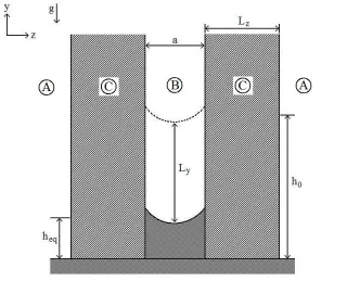
Figure 2.1 Theoretical setup for Hele-Shaw cell partially submerged in silicone oil, front and side view. Shows equilibrium height based on hydrostatic and capillary pressures,heq, as well as equilibrium height for hydrostatic, elec-trohydrostatic and capillary pressures, h0. Also displays span-wise length
b and plate separation distance a. Indicates thickness of glass plates,Lz,
and range of actuation, Ly. . . 4 Figure 2.2 Breakdown of the Hele-Shaw cell into three primary regions: (A)
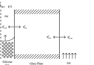
repre-sents external natural convection, (B) reprerepre-sents internal forced convec-tion and (C) represents solid wall conducconvec-tion. . . 5 Figure 2.3 Boundary conditions balancing the heat flux into and out of the wall on
the inner surface and outer surface. . . 7
Figure 3.1 Experimental setup demonstrating connection of Hele-Shaw cell to power source in the front view as well as relative camera and temperature probe positions with the side view. . . 9 Figure 3.2 Translation of image data into a calculation of the interface height; (a)
shows default image, (b) shows marked pixels due to pixel brightness greater than a set threshold and (c) shows final interface outline deter-mined by MATLAB code. . . 11 Figure 3.3 Temperature data for an experimental set using a 2 second actuation
period and a hotplate temperature of 50 ◦C. . . 11 Figure 3.4 Temperature data for an experimental set using a 20 second actuation
period and a hotplate temperature of 50 ◦C. . . 12 Figure 3.5 Temperature data for an experimental set using a 200 second actuation
period and a hotplate temperature of 50 ◦C. . . 12 Figure 3.6 Temperature data for an experimental set using a 2 second actuation
period and a hotplate temperature of 75 ◦C. . . 13 Figure 3.7 Temperature data for an experimental set using a 20 second actuation
period and a hotplate temperature of 75 ◦C. . . 13 Figure 3.8 Temperature data for an experimental set using a 200 second actuation
period and a hotplate temperature of 75 ◦C. . . 14 Figure 3.9 Temperature probe position versus the mean temperature rise for each
experimental set with a hotplate temperature of 50 ◦C. . . 15 Figure 3.10 Temperature probe position versus the mean temperature rise for each
experimental set with a hotplate temperature of 75 ◦C. . . 15 Figure 3.11 Overview of mean temperature rise for each actuation period and both
hotplate temperatures. . . 16 Figure 3.12 Dimensionless mean temperature rise versus the dimensionless group of
the inverse of the product of the Strouhal and P´eclet numbers. . . 17
Figure 3.13 Experimentally observed periodic rise heights for a 2 second actuation period and both hotplate temperatures of 50 ◦C and 75 ◦C. . . 18
Figure 4.1 Formation of a thin film on the glass plates after the silicone oil-air in-terface recedes from an initial height determined by the applied electric field. . . 20
Figure 5.1 Experimental setup with a silicone oil viscosity of 1000 cSt and plate separation distance of 300 µm. . . 24 Figure 5.2 Interface images for (a) base equilibrium height before actuation, (b)
max-imum rise hight during actuation, (c) interface as it falls from the maxi-mum rise height and (d) the base equilibrium height after actuation. The top image set corresponds to a plate separation distance of 500 µm with 100 cSt silicone oil while the bottom set corresponds to a plate separation distance of 300 µm with 1000 cSt silicone oil. . . 24 Figure 5.3 Ratio of electrostatic Bond number and hydrostatic Bond number Bo
∗
E
Bo∗H
versus a ratio of the relative rise height to plate separation distance h0−heq
a
compared with theoretically expected values. . . 25 Figure 5.4 Observed data from an experimental set with a plate separation distance
of 500 µm and a silicone oil viscosity of 100 cSt as well as an applied volt-age of 1200 V compared with theoretical values for an analytical solution with zero film thickness. . . 26 Figure 5.5 Dimensional interface height data for a rise height comparison with 750
µm plate separation distance and 1000 cSt silicone oil viscosity. . . 27 Figure 5.6 Dimensionless interface height data for a rise height comparison with 750
µm plate separation distance and 1000 cSt silicone oil viscosity. . . 27 Figure 5.7 Dynamic film thickness data versus time for a rise height comparison with
750µm plate separation distance and 1000 cSt silicone oil viscosity. . . . 28 Figure 5.8 Dynamic film thickness data versus capillary number for a rise height
comparison with 750 µm plate separation distance and 1000 cSt silicone oil viscosity. . . 28 Figure 5.9 Dimensional interface height data for a viscosity comparison with 500µm
plate separation distance and an applied electrical potential of 1200 V. . . 29 Figure 5.10 Dimensionless interface height data for a viscosity Comparison with 500
µm plate separation distance and an applied electrical potential of 1200 V. 30 Figure 5.11 Dynamic film thickness data versus time for a viscosity comparison with
500 µm plate separation distance and an applied electrical potential of 1200 V. . . 30 Figure 5.12 Dynamic film thickness data versus capillary number for a viscosity
com-parison with 500 µm plate separation distance and an applied electrical potential of 1200 V. . . 31 Figure 5.13 Dimensional interface height data for a gap spacing comparison with 10
cSt silicone oil viscosity. Used 2400 V forBo∗H = 0.33, 1800 V forBo∗H = 0.15 and 1200 V for Bo∗H = 0.053. . . 31
Figure 5.14 Dimensionless interface height data for a gap spacing comparison with 10 cSt silicone oil viscosity. Used 2400 V forBo∗H = 0.33, 1800 V forBo∗H = 0.15 and 1200 V for Bo∗H = 0.053. . . 32 Figure 5.15 Dynamic film thickness data versus time for a gap spacing comparison
with 10 cSt silicone oil viscosity. Used 2400 V forBo∗H = 0.33, 1800 V for
Bo∗H = 0.15 and 1200 V for Bo∗H = 0.053. . . 32 Figure 5.16 Dynamic film thickness data versus capillary number for a gap spacing
comparison with 10 cSt silicone oil viscosity. Used 2400 V forBo∗H = 0.33, 1800 V forBo∗H = 0.15 and 1200 V for Bo∗H = 0.053. . . 33 Figure 5.17 Initial film thickness from asymptotic solution plotted against initial
cap-illary number with curve fits based on Eq. 5.2. Subplot insert shows con-stant film thickness from analytical solution against initial capillary number. 34
Figure A.1 Observed periodic interface motion for the hotplate temperature of 50◦C for a 2 second actuation period. . . 40 Figure A.2 Observed periodic interface motion for the hotplate temperature of 50◦C
for a 20 second actuation period. . . 40 Figure A.3 Observed periodic interface motion for the hotplate temperature of 50◦C
for a 200 second actuation period. . . 41 Figure A.4 Observed periodic interface motion for the hotplate temperature of 75◦C
for a 2 second actuation period. . . 41 Figure A.5 Observed periodic interface motion for the hotplate temperature of 75◦C
for a 20 second actuation period. . . 42 Figure A.6 Observed periodic interface motion for the hotplate temperature of 75◦C
for a 200 second actuation period. . . 42 Figure A.7 Mean temperatures for an experimental set (TH = 75 ◦C, 2 second
ac-tuation period) where the dashed lines represent mean temperature; TA
is mean temperature before actuation, TB is mean temperature during
actuation and TC is mean temperature after actuation. . . 44
Chapter 1
Introduction
The purpose of this research is to investigate the potential of an electrically actuated micro-scale single phase heat transfer device with no moving parts. A device of this variety may be
useful in operating in areas where space is limited and heat transfer is necessary. With industry
progressing the way it is, there is an increased interest in enhancing heat transfer in micro-scale geometries. In these micro-micro-scale geometries, there are several methods of producing heat
transfer devices. The first of which is a two-phase heat exchanger, in which the working fluid
generates large amounts of heat transfer through latent heat of transformation, moving from a liquid phase to a solid phase. The less dense gaseous phase then transfers to an area with less
heat and condenses, releasing the energy in another area [7, 6]. One of the limitations associated
with this model is that the heat exchanger only operates between specific temperature ranges required for phase transition [2]. This limitation can be overcome using a single-phase heat
exchanger which requires some method of actuation for the working fluid to generate increased
heat exchange.
In most situations, actuation of the working fluid is achieved by using some sort of pump
to generate a pressure differential that will induce motion of the working fluid. This is most
commonly achieved using a pump and inputting work to generate the pressure difference. Some research has been done in an effort to increase the heat transfer by applying high-frequency
oscillations to the flow [5, 8], somewhat similar to pulsating heat pipes based on two-phase
work-ing fluid. However, in micro-scale geometries, it is possible to generate actuation of particular fluids by inducing an electrical voltage over an area, generating electrohydrostatic pressures
[11, 12]. The properties of silicone oil are favorable in this regard as the oil is relatively
in-compressible and poorly conducting, allowing the actuation of the interface due to the electric field [4, 11] This provides an advantage in limited geometries by inducing actuation of a fluid
without the use of moving parts, potentially increasing heat exchange in an area where space is at a premium. The actuation can be controlled by a function generator to induce periodic
actuation of the working fluid.
This thesis explores the possibility of generating a heat dissipation device in a micro-scale geometry that operates by induced electrical fields causing actuation of fluids. In order to assess
the potential of such a device, the mechanics of it need to be analyzed and tested using a similar
model. Here, a vertical Hele-Shaw cell is constructed using indium-tin-oxide (ITO) coated glass plates. Glass plates are chosen for transparency so that fluid motion can be accurately observed
during actuation. The plates are coated with ITO so that the plates can carry an electric voltage,
allowing the Hele-Shaw cell to act as a capacitor when connected with a voltage source. Silicone oil is chosen as the primary working fluid due to its favorable electrical properties, which allow
actuation when place within an electric field.
Figure 1.1: The proposed Hele-Shaw cell device partially submerged in a beaker of silicone oil.
This proposed device allows fluid motion within a micro-scale channel. As such, there are
several assumptions that can be made to simplify a theoretical analysis. The separation distance
between the glass plates is small relative to the width of the plates, such that we can assume there is no significant effect due to the side walls of the Hele-Shaw cell. The flow that will be
induced using the electrical field is assumed to be both low Reynolds number flow and low
capillary number flow. As stated, the separation distance between the glass plates is small, such that the corresponding hydrostatic Bond number is assumed to be small as well.
Chapter 2
Heat Transfer Theory
The proposed device for analysis is a vertical Hele-Shaw cell placed within a reservoir of sili-cone oil. The silisili-cone oil rises to a base equilibrium height based on hydrostatic and capillary
pressures. Capillary pressures are due to wetting between the fluid and the surface of the glass
plates that make up the Hele-Shaw cell. Here, we assume that there are no wall effects in the x-direction. This is due to the relative distance between the walls of the Hele-Shaw cell, b,
when compared with the plate separation distance, a. This assumption allows us to reduce the
problem to 2 dimensions, focusing on the change in position of the interface in the y-direction and heat transfer in the z-direction. Actuation of the fluid interface is achieved using an
elec-trical voltage to produce electrohydrostatic pressure in addition to capillary and hydrostatic
pressures.
In order to investigate the potential of this device, a model is devised in which the heat
transfer potential can be determined. The model developed here is based on the time dependent
heat conduction equation. For this particular setup, the model is symmetric, such that the time dependent heat conduction equation is applied to one of the plates of glass used in the
Hele-Shaw cell. There are three regions to be considered as shown in Figure 2.2; the glass plate, the
interior of the Hele-Shaw cell and the exterior of the Hele-Shaw cell.
In this model, we assume forced convection within the interior of the Hele-Shaw cell,
con-duction within the glass plate and natural convection along the exterior of the Hele-Shaw cell.
This model focuses on the conduction within the glass plates and takes the interior and exterior conduction into the boundary conditions of the problem.
∂T ∂t =αs
∂2T
∂z2 (2.1)
Figure 2.1: Theoretical setup for Hele-Shaw cell partially submerged in silicone oil, front and side view. Shows equilibrium height based on hydrostatic and capillary pressures,heq, as well as
equilibrium height for hydrostatic, electrohydrostatic and capillary pressures, h0. Also displays span-wise length band plate separation distance a. Indicates thickness of glass plates,Lz, and range of actuation, Ly.
2.1
Time-dependent Conduction Analysis
The time-dependent conduction equation is initially made to be dimensionless for further
un-derstanding. The temperature is made dimensionless using the temperature of the ambient air
as well as the maximum mean temperature of the working fluid within the Hele-Shaw cell. The solution focuses on one dimension initially in order to produce a working model at a
pre-determined height. As the oil-air interface is oscillating during actuation, there is a range of
motion that the interface is active over. Due to the limitations of heating the internal fluid, this produces a range of mean fluid temperatures that the interior of the Hele-Shaw device
can experience. The maximum mean fluid temperature here is the largest mean temperature
experienced by the interior of the Hele-Shaw cell at a prescribed initial vertical height.
∂θ ∂t∗ =
αs L2
zω ∂2θ ∂z∗2 =
1 (St)(P e)
∂2θ
∂z∗2 (2.2)
Once the time-dependent conduction equation is made dimensionless, two particular
di-mensionless numbers appear to come into play. The temperature distribution appears to be
a function of the Strouhal and P´eclet numbers. Both these dimensionless numbers take into consideration the mean fluid velocity and the plate separation distance. The P´eclet number
Figure 2.2: Breakdown of the Hele-Shaw cell into three primary regions: (A) represents exter-nal natural convection, (B) represents interexter-nal forced convection and (C) represents solid wall conduction.
also involves the thermal conduction constant and reflects the effect of the constant on the
tem-perature distribution. The Strouhal number takes into consideration the oscillation frequency of the forced convection, reflecting the effect of the frequency on the temperature distribution.
2.2
Boundary Condition Analysis
The time-dependent heat conduction equation is solved using discretization methods; first order Euler in time and first order central difference in space. Of note to this solution is the choice of
boundary conditions. For this particular setup, the outer surface of the glass plate is assumed to be natural convection in air. The inside surface of the glass plate is exposed to forced
convection within a channel. The flow within the channel is determined from theory based on
the periodically applied electrical potential and used for the internal forced convection. Also for the internal forced convection, there are two working fluids, being the silicone oil and the air,
depending on the location chosen for observation (assumed within the range of actuation).
∂θ ∂z∗ =
hLz
ks (θw−θf) =Bi(θw−θf) (2.3)
In setting up the boundary conditions for this discretization, another dimensionless number becomes evident; the Biot number. Here, the Biot number appears to reflect the amount of heat
transferred by conduction at the boundary compared with the amount of heat transferred by
convection. This Biot number provides a reflection on the efficiency of the convective process to transfer heat to, or from, a particular solid. There is then a Biot number associated with each
boundary condition, the first into the fluid within the Hele-Shaw cell, the second in relation to
the natural convection on the outer surface of the Hele-Shaw cell.
Figure 2.3: Boundary conditions balancing the heat flux into and out of the wall on the inner surface and outer surface.
Chapter 3
Heat Transfer Experiment
Experiments are performed to understand the dynamics of the fluid flow within the Hele-Shaw cell and the temperature dissipation potential of the periodic interface actuation. 76
experiments are performed in order to measure the temperature rise due to actuation of a
silicone oil within the Hele-Shaw cell. Dynamics of the periodic flow are observed as well as temperature fluctuations over the course of the experiments.
3.1
Heat Transfer Experimental Setup
The device is based around the electrohydrostatic effect that is possible in silicone oils within small geometries. For this experiment, two ITO (indium-tin-oxide) coated glass plates are setup
with precision spacers between them in order to form a vertical Hele-Shaw cell type system.
The working fluid is a silicone oil with a density of 960 kg/m3. Silicone oil is chosen due to the favorable electrical properties that it possesses. Note for this setup that air is a secondary
working fluid as the gap spacing between the glass plates is filled with silicone oil due to capillary and hydrostatic pressures (and later electrohydrostatic pressure) and otherwise filled with air.
The Hele-Shaw cell is held together using paper clips and then attached using alligator clips
to a power supply through a function generator. The power supply and function generator are used to supply an electrical potential to the Hele-Shaw cell in order to induce actuation of
the oil-air interface. The actuation distance is based on the hydrostatic Bond number and the
electrostatic Bond number of the device. The function generator is used to apply the voltage at a periodic interval in order to induce oscillatory motion of the oil-air interface. This actuation
of the oil-air interface is done in order to increase the convective heat transfer between the glass
plates in an effort to increase the effective heat transfer of the device.
The Hele-Shaw cell is placed in a reservoir (glass beaker) of silicone oil with a viscosity of 10
cSt. The silicone oil rises between the glass plates due to hydrostatic and capillary pressures, up
to an initial oil-air interface equilibrium height. The glass beaker is place on top of a hot plate
which is used to increase the temperature of the oil. Once the oil-air interface has reached an equilibrium height, a CCD camera is used to take a picture of the setup and acquire a reference
of the equilibrium height of the oil-air interface. Then the periodic electrical potential is applied
to the Hele-Shaw cell and the oil-air interface begins to oscillate. During this oscillation of the oil-air interface, the CCD camera is used to take a video of the motion so that the dynamics
of the oil-air interface can be determined. A dark background is achieved by placing a piece
of black cardboard behind the Hele-Shaw cell. This, combined with a light used to increase brightness of the silicone oil-air interface allows for easier reading of the interface position.
Figure 3.1: Experimental setup demonstrating connection of Hele-Shaw cell to power source in the front view as well as relative camera and temperature probe positions with the side view.
Temperature probes are set on the side of the glass (outside and exposed to natural
vection) in order to measure the surface temperature of the surface of the Hele-Shaw cell.
Temperature data is recorded before actuation in order to acquire a base line for the tempera-ture distribution and then both during and after actuation in order to determine the effect of
actuation on heat transfer. This temperature data is then analyzed using MATLAB in order
to determine the mean temperature experienced by the surface of the Hele-Shaw cell. These values are to be compared with a theoretical model.
In order to analyze the effect of actuation on heat dissipation, several sets of experiments
are performed using the 750µm plate separation distance with a silicone oil of 10 cSt viscosity. Here, the same voltage magnitude is applied for each experiment using a square waveform with
a period of 2, 20 and 200 seconds. This maintains the same relative rise height, allowing for a
relatively constant range of actuation for each experimental set. The same experiments are run for two different fluid temperatures, based on heat generated by the hot plate. Here, video data
is taken for a set time period to observe the dynamics of actuation. Additionally, temperature
data is recorded from two temperature probes in contact with the outer surface of the Hele-Shaw cell, located around the region of actuation.
3.2
Heat Transfer Experimental Results
The image, video and temperature data are analyzed using MATLAB code written to determine
interface height and surface temperature over time. Interface position is determined from image
and video data by measuring the average location of the interface over the range of the Hele-Shaw cell. This measurement is accomplished by recording the pixels indicating the interface
with a larger light/color value. The number of pixels are summed in the x-direction for each
line in the y-direction. The value number of pixels per line are then multiplied by the height of the line and added together. This value is then divided by the total number of pixels in order
to obtain the average position of the interface in the y-direction, i.e. the height of the interface.
In addition to the height data, velocity data is acquired by performing a simple measurement of the difference in height divided by the difference in time over the experiment.
For the analysis of the temperature data, two temperature probes record temperature data
at different heights for three different actuation frequencies and two separate fluid temper-atures. For each experimental set, a silicone oil with a viscosity of 10 cSt is used. The plate
separation distance for the Hele-Shaw cell is 750µm. Multiple sets are run for each temperature
and frequency to gather additional sample points to account for the variation in temperature readings. The first temperature is set by setting the hotplate to 50◦C. The second temperature
is acquired by setting the hotplate to a temperature of 75 ◦C. The hotplate temperature, TH, is used to obtain the dimensionless temperature,
Figure 3.2: Translation of image data into a calculation of the interface height; (a) shows default image, (b) shows marked pixels due to pixel brightness greater than a set threshold and (c) shows final interface outline determined by MATLAB code.
θ= T−T∞
TH −T∞
. (3.1)
However, the hotplate temperature is not equivalent to the temperature of the fluid operating
within the actuation range of the Hele-Shaw cell due to natural conduction and convection into
the ambient air.
Figure 3.3: Temperature data for an experimental set using a 2 second actuation period and a hotplate temperature of 50 ◦C.
Figure 3.4: Temperature data for an experimental set using a 20 second actuation period and a hotplate temperature of 50 ◦C.
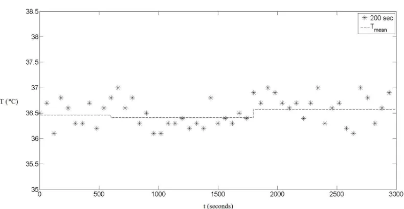
Figure 3.5: Temperature data for an experimental set using a 200 second actuation period and a hotplate temperature of 50 ◦C.
Figure 3.6: Temperature data for an experimental set using a 2 second actuation period and a hotplate temperature of 75 ◦C.
Figure 3.7: Temperature data for an experimental set using a 20 second actuation period and a hotplate temperature of 75 ◦C.
Figure 3.8: Temperature data for an experimental set using a 200 second actuation period and a hotplate temperature of 75 ◦C.
Figure 3.3 through Figure 3.8 show experimental temperature data obtained for both
hot-plate temperatures and each of the three actuation periods. For each experiment, 10 minutes or
600 seconds is allowed to acquire a baseline temperature for the corresponding probe position. Actuation then begins with the corresponding frequency and is allowed to continue for
approxi-mately 20 minutes or 1200 seconds. Afterwards, temperature data is collected for an additional
20 minutes for comparison to the previous baseline temperature. Temperature rise during actu-ation is calculated by taking the mean temperature of the data 60 seconds after actuactu-ation was
initiated. This mean temperature is compared with the mean temperatures before actuation
and 60 seconds after actuation is halted, giving ∆T, which is used to approximate temperature rise due to actuation. Additionally, the location of each temperature probe is recorded relative
to the base interface height achieved during actuation, recorded as y =h−heq. Comparisons
of each ∆T associated with a particular y position are computed and displayed in Figure 3.9 and Figure 3.10 as well.
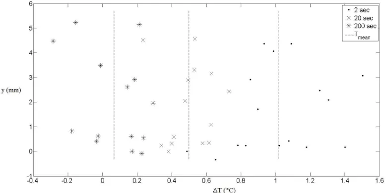
Dimensionless temperature probe location is determined by using the range of actuation for
each set,Ly =h0−heq, withh0 being the maximum interface height achieved during actuation. The dimensionless probe location is then calculated as follows,
y∗ = h−heq
h0−heq
. (3.2)
The temperature rise and the corresponding probe location are made dimensionless for
Figure 3.9: Temperature probe position versus the mean temperature rise for each experimental set with a hotplate temperature of 50 ◦C.
Figure 3.10: Temperature probe position versus the mean temperature rise for each experi-mental set with a hotplate temperature of 75 ◦C.
parison between the different hotplate temperature values. In addition to this calculation, the
mean temperature rise is obtained for each group of experimental sets with the same actuation period and hotplate temperature. These values, including the mean temperature rise, are shown
in Figure 3.11.
Figure 3.11: Overview of mean temperature rise for each actuation period and both hotplate temperatures.
3.3
Heat Transfer Experiment Discussion
From results of the temperature data, there is an observable temperature rise due to actuation
of a heated silicone fluid within a Hele-Shaw cell. There does not appear to be a dependence of the temperature rise on the position of the temperature probe, indicating that the
temper-ature rise is relatively the same regardless of position within the range of actuation. Following this, the mean temperature rise is determined for each of the experimental sets based on
ac-tuation frequency and hotplate temperature. These mean temperatures are plotted against the
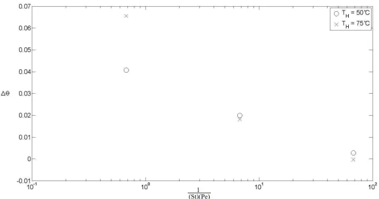
dimensionless group of Strouhal and P´eclet numbers, as shown in Figure 3.12.
Figure 3.12 shows dimensionless temperature rise against the dimensionless group of the
inverse of the product of the Strouhal and P´eclet numbers. Here, there is a relationship between
the temperature rise and the dimensionless group such that a smaller dimensionless group yields a larger temperature rise. Note that there is a limit to this based on the actuation frequency. As
Figure 3.12: Dimensionless mean temperature rise versus the dimensionless group of the inverse of the product of the Strouhal and P´eclet numbers.
the actuation frequency increases, the range of actuation starts to decrease. Beyond a particular
point, the actuation frequency is too large for the interface to approach the corresponding
equilibrium heights, and the range of actuation approaches zero. Note also that there appears a difference in the dimensionless temperature rise between the two hotplate temperatures used
at the lowest value of the inverse of the product of Strouhal and P´eclet numbers. Here, we see
a larger temperature rise for the higher hotplate temperature. This is likely due to changes in the fluid properties due to the higher fluid temperature, potentially affecting viscosity which
may in turn affect the formation of a film on the plate walls.
Figure 3.13 shows a comparison of the 2 second actuation period between the two observed hotplate temperatures. The higher temperature fluid flow appears to approach the equilibrium
position faster than the lower temperature flow. This difference helps to demonstrate the change
in fluid properties from the lower hotplate temperature to the higher hotplate temperature. The increase in fluid velocity might be attributed to a decrease in the silicone oil viscosity, which
yields an increase in the heat transfer [10] which is observed in Figure 3.12. In addition to this
observation, a likely concern to the heat dissipation potential of the device is the film thickness formation during the down stroke, as it will have an effect on the heat transfer of the device
[3, 10].
Figure 3.13: Experimentally observed periodic rise heights for a 2 second actuation period and both hotplate temperatures of 50◦C and 75 ◦C.
Chapter 4
Thin Film Theory
Considering that the formation of a thin film on the boundary of the plates may have significant effects to the heat transfer of the device, we shift focus to the formation of the thin film during
the recession of the interface from the glass plates. Research has been done comparing film
thickness to capillary number in cases where the plate is moving [14] and where there is a fluid penetrating the gap spacing [1, 9]. So, our focus will be into the relationship between the film
thickness, s, and the capillary number Ca∗, where Ca∗ = µL
γ dh dt.
In this theory, additional assumptions are made in regards to the thin film. Figure 4.1 shows the assumed formation of the thin film on the glass plate after the interface recedes from an
initial equilibrium height due to electrohydrostatic and capillary pressures.
Here, we assume here that the pressure gradient is dependent only on time. In regards to the film itself, we assume here that film thickness remains constant along the side of the plate
wall. This assumption is used to define the active plate separation distance as the actual plate
separation distance minus the thin film formed on both sides of the Hele-Shaw cell, a−2s. These assumptions are in addition to the assumptions of low capillary and Bond numbers.
Bond number is obtained as Bo∗H = (`a
c)
2 where`c is the capillary length given by`c=qγ ρg.
4.1
Mass and Momentum Conservation Analysis
First, we begin with defining the flux of the interface, q. Considering the assumption of a film
thickness constant along the side of the wall, we subtract the distance from the plate separation distance for the active area. This yields the flux of the interface asq = dhdt(a−2s), which will be used for the analysis. Next, analysis into the formation of a thin film on the walls of the glass
plates proceeds with the momentum equation,
ρL
∂v
∂t +v·∇v
=∇·σ. (4.1)
Figure 4.1: Formation of a thin film on the glass plates after the silicone oil-air interface recedes from an initial height determined by the applied electric field.
The momentum equation is solved based on the assumptions that have been made here.
The velocity function is obtained based on boundary conditions of zero slope in the center of the interface, ∂v∂x = 0 atx= a2, and zero velocity at the boundary of the film,v= 0 atx=s(t).
v(x, t) = pz 2µL
(x2−a(x−s)−s2) (4.2)
Next, the velocity equation is used with the equation for the net flux in order to obtain a relationship between dhdt and a function ofs as follows,
q= dh
dt(a−2s) =
Z a−s
s
v(x, t)dx= 2
Z a/2
s
v(x, t)dx (4.3)
dh dt = pz µL β (4.4) where,
β = 1 12
−a3+ 6a2s−12as2+ 8s3
a−2s (4.5)
This net flux provides a solution relating the average interface velocity with a parameterβbased
on the plate separation distance, a, and the film thickness, s. This equation is then integrated
in order to obtain the static pressure. The interfacial stress is then used to obtain a solution relating the capillary number with interface height and the film thickness, assuming no shear
stress contribution.
−Ca∗ =−µL
γ dh dt =β
2
a−2s
1 h− 1 `2 c (4.6)
4.2
Asymptotic Limit Analysis
We then use this solution in order to obtain an equation for the film thickness itself. Due to the difficulty in achieving a direct solution for the film thickness from this equation, asymptotic
limits are used in order to obtain an approximate solution. First, Eq. 4.6 is expanded and set to equal zero, such that sappears in a quadratic polynomial.
C1s2+C2s+C3 +[−83(`1
c)
2s2+ (a `2
c −
2
h)s+ 4Ca ∗−1
6Bo
∗ H]as + [
2 3(
1
`c)
2s2+4 3 1
hs+ 4Ca ∗](s
a)2= 0
(4.7)
where,
C1 = 1
`2
c
(4.8a)
C2 = 1
h − a
2`2
c
(4.8b)
C3 =
Bo∗H
12 −
a
6h +Ca ∗
. (4.8c)
In order to obtain a solution, we assume that the ratio of the film thickness to the plate
separation distance, as, is very small, such that the ratio can be neglected as well as the ratio squared (sa)2. Using this assumption along with the assumption of low Bond numbers, Eq. 4.7 is reduced to a simple quadratic polynomial in terms of the film thicknesssand the associated
constants,C1,C2 and C3. This is solved for the following relationship,
s(t) =−1 2 C2 C1 ± s 1 4 C2 C1 2
−C3
C1
(4.9)
4.3
Analytical Solution for Constant Film Thickness
This solution gives an approximation for the film thickness over time; however, an analytical
solution for the film thickness is possible if the film thickness is assumed to be constant at
later times, which is analogous to the Washburn solution [13]. This analytical solution gives an approximation for the constant film thickness after the initial dynamics have dissipated.
β `2
c γ µL
∆t=heqln
heq−h heq−h0
+ (h−h0). (4.10)
Both the asymptotic limit solution and the analytical solution will be useful in analyzing
the effects of Bond number, capillary number and initial rise height on the formation of a thin
film on the glass plates. The asymptotic limit solution provides an approximation of the film thickness with respect to time, while the analytical solution provides an approximation of the
film thickness as a constant at later times.
Chapter 5
Thin Film Experiment
Additional experiments are run to better understand the thin film formation. 24 experimental sets are run for various silicone oil viscosities, plate separation distances and initial rise heights.
These experiments are compared with both the asymptotic approximation for dynamic film
thickness as well as the analytical solution for a constant film thickness at later times.
5.1
Thin Film Experimental Setup
The experimental setup used here is similar to the experimental setup used for the temperature
analysis. The Hele-Shaw cell is set up and placed within the silicone oil reservoir in the same manner along with the camera to record interface position as shown in Figure 5.1. Here, an
analysis is done on silicone oil of viscosity 10, 100 and 1000 cSt, as well as plate separation
distances of 300, 500 and 750 µm and three different electrical voltages (based on the plate separation distance). These variables are used to determine which parameters affect the thin
film formation.
Initially, the setup is allowed to reach the initial equilibrium height based on hydrostatic and
capillary pressures,heq. An image is taken and an electrical voltage is applied to the Hele-Shaw
cell. The interface is allowed to reach a new equilibrium height based on the hydrostatic, cap-illary and electrohydrostatic pressures,h0. Here, video data begins recording and the electrical
potential is removed, causing the interface to recede and leave a thin film on the side of the glass
plates. The interface position is recorded in the video data until the interface appears to reach a new equilibrium position without the electrohydrostatic pressure as shown in Figure 5.2. The
same MATLAB code is used to extract interface position with respect to time based on the
video data obtained.
Figure 5.1: Experimental setup with a silicone oil viscosity of 1000 cSt and plate separation distance of 300µm.
a
b
c
d
Figure 5.2: Interface images for (a) base equilibrium height before actuation, (b) maximum rise hight during actuation, (c) interface as it falls from the maximum rise height and (d) the base equilibrium height after actuation. The top image set corresponds to a plate separation distance of 500 µm with 100 cSt silicone oil while the bottom set corresponds to a plate separation distance of 300µm with 1000 cSt silicone oil.
5.2
Thin Film Experimental Results
Data obtained from these experiments is analyzed with respect to theory. First off, we look over
the theoretical rise heights and compare these values with experimentally observed rise heights. This is accomplished by comparing the hydrostatic Bond number,Bo∗H, with the electrostatic Bond number, Bo∗E. The hydrostatic Bond number is obtained as Bo∗H = (`a
c)
2, while the
electrostatic Bond number is obtained as Bo∗E = ∆φ2a2. The ratio of the electrostatic Bond number to the hydrostatic Bond, Bo
∗
E
Bo∗H, is compared with
h0−heq
a . The relationship that we
theoretically expect to observe is a slope of 1 between these values. Figure 5.3 shows the
resulting observed results versus a theoretical slope.
Figure 5.3: Ratio of electrostatic Bond number and hydrostatic Bond number Bo ∗
E
Bo∗H versus a
ratio of the relative rise height to plate separation distance h0−heq
a compared with theoretically
expected values.
For the most part, experimentally observed rise heights correspond well with expected
the-oretical values. The primary differences occur for the smallest plate separation distance, cor-responding with Bo∗H = 0.053. This is likely due to experimenter error. The time required to reach an equilibrium height increases drastically with decreasing plate separation distance.
It is probable that the experimenter did not allow sufficient time for the interface to reach a new equilibrium height after applying the electrical field, meaning that the observed initial rise
height is lower than theoretically expected. This discrepency should not have any effect on the
rest of the results as the theory uses the observed initial rise height rather than the theoretical
initial rise height.
Continuing the analysis of the data produced from these experiments, we compare
experi-mentally observed data with theoretical data in which no film forms. This is accomplished by
solving the analytical solution for a constant film thickness at later times for an expected film thickness of zero. This analysis is done in an attempt to determine whether or not a thin film
forms and the subsequent effect on the interface dynamics. Figure 5.4 shows the analysis of
interface height data and interface velocity data for one of the experimental sets.
Figure 5.4: Observed data from an experimental set with a plate separation distance of 500
µm and a silicone oil viscosity of 100 cSt as well as an applied voltage of 1200 V compared with theoretical values for an analytical solution with zero film thickness.
For the analysis of film formation, several comparisons are performed. The first analysis is
based on a constant film thickness approximation. For this analysis, the analytical solution for
film formation is solved assuming a constant film thickness. In order to obtain this solution, the initial interface location is matched to the equation and a constant film thickness is chosen such
that the final theoretical interface height matches the experimental data. This process provides
us with a theoretical solution with a constant film thickness for comparison with experimentally observed data. The second analysis involves the calculation of a dynamic film thickness based
on the asymptotic approximation for the film thickness formation. For this comparison the
experimental interface height data is used to determine the film thickness over time.
Figure 5.5: Dimensional interface height data for a rise height comparison with 750µm plate separation distance and 1000 cSt silicone oil viscosity.
Figure 5.6: Dimensionless interface height data for a rise height comparison with 750µm plate separation distance and 1000 cSt silicone oil viscosity.
Figure 5.7: Dynamic film thickness data versus time for a rise height comparison with 750µm plate separation distance and 1000 cSt silicone oil viscosity.
Figure 5.8: Dynamic film thickness data versus capillary number for a rise height comparison with 750µm plate separation distance and 1000 cSt silicone oil viscosity.
Several comparisons are performed from the data obtained for each experimental set. These
comparisons provide insight into the effect of various parameters on the formation of a thin film on the surface of the wall. Figure 5.5 through Figure 5.8 shows a comparison of applied electrical
voltages, generating three different initial rise heights. Figure 5.9 through Figure 5.12 shows a
comparison of silicone oil viscosity. Figure 5.13 through Figure 5.16 shows a comparison of the three plate separation distances, displayed using the corresponding Bond numbers. Maintaining
similar rise heights for the plate separation distance comparison is attempted using an applied
electrical voltage based on the maximum voltage that the plate separation distance could endure before the air breaks down and begins to transmit charge from one plate to the other.
Figure 5.9: Dimensional interface height data for a viscosity comparison with 500 µm plate separation distance and an applied electrical potential of 1200 V.
5.3
Thin Film Experiment Discussion
From the dynamic film thickness calculation, several parameters can be examined. Figure 5.17
shows a comparison of the initial maximum film thickness versus the initial maximum capillary number for each experimental set. These values indicated a trend that was apparent in the
initial film thickness against both initial capillary number and the hydrostatic Bond number.
Using an exponential curve fit, a basic form for the relationship between initial film thickness with initial capillary number and hydrostatic Bond number is determined as
Figure 5.10: Dimensionless interface height data for a viscosity Comparison with 500µm plate separation distance and an applied electrical potential of 1200 V.
Figure 5.11: Dynamic film thickness data versus time for a viscosity comparison with 500 µm plate separation distance and an applied electrical potential of 1200 V.
Figure 5.12: Dynamic film thickness data versus capillary number for a viscosity comparison with 500µm plate separation distance and an applied electrical potential of 1200 V.
Figure 5.13: Dimensional interface height data for a gap spacing comparison with 10 cSt sili-cone oil viscosity. Used 2400 V forBo∗H = 0.33, 1800 V for Bo∗H = 0.15 and 1200 V forBo∗H = 0.053.
Figure 5.14: Dimensionless interface height data for a gap spacing comparison with 10 cSt silicone oil viscosity. Used 2400 V forBo∗H = 0.33, 1800 V forBo∗H = 0.15 and 1200 V for Bo∗H
= 0.053.
Figure 5.15: Dynamic film thickness data versus time for a gap spacing comparison with 10 cSt silicone oil viscosity. Used 2400 V forBo∗H = 0.33, 1800 V forBo∗H = 0.15 and 1200 V for
Bo∗H = 0.053.
Figure 5.16: Dynamic film thickness data versus capillary number for a gap spacing comparison with 10 cSt silicone oil viscosity. Used 2400 V for Bo∗H = 0.33, 1800 V for Bo∗H = 0.15 and 1200 V forBo∗H = 0.053.
s∗0= 1 2
h
1−ec1Ca∗0
i
. (5.1)
Here, initial film thickness corresponds to an exponential term with an unknown constant,c1,
and the initial capillary number,Ca∗0. Using a best fit for each set of experimental data belong-ing to a particular Bond number, values are obtained forc1. By comparing the values forc1 to
the corresponding Bond numbers, the relationship is further refined as
s∗0 = 1 2
"
1−ec2
Ca∗0 Bo∗ H
#
. (5.2)
This relation appears to indicate that the initial film thickness corresponds to the ratio of the
initial capillary number and the hydrostatic Bond number. Performing a best fit curve with
this relationship yields a value of c2 = 6450 for each experimental set.
Figure 5.17: Initial film thickness from asymptotic solution plotted against initial capillary number with curve fits based on Eq. 5.2. Subplot insert shows constant film thickness from analytical solution against initial capillary number.
Chapter 6
Conclusions
In this study, an electrically actuated micro-scale single-phase heat transfer device has been proposed and analyzed. The device used a Hele-Shaw cell made of coated glass plates acting as
a capacitor in order to actuate a silicone oil-air interface by use of an electric field controlled
with a function generator. Experiments are conducted to examine the potential for such a device using a 10 cSt silicone oil reservoir heated by a hotplate. Two hotplate temperatures are used
to vary the temperature of the silicone oil. Multiple actuation frequencies are also examined.
Overall, experimental results indicate that periodic actuation of a heated silicone oil by means of electric voltage generates a temperature rise over the range of actuation for a
suffi-ciently high actuation frequency. Temperature rise is observed to be independent of position
within the range of actuation, so mean temperature rise is the same over the range of actuation. The temperature of the silicone oil used in actuation appears to affect the resulting
dimension-less temperature rise, which may indicate some dependence of the dimensiondimension-less temperature
rise on the formation of a thin film from the silicone oil.
The change in tempearture of the silicone oil may have an effect on the viscosity of the
silicone oil, as changes in interface velocity are observed for the same periodic actuation. These
changes appear to result in an increase in the dimensionless temperature rise as the silicone oil temperature increases. Due to this possibility, experiments are performed to analyze the effect
of viscosity, plate separation distance and rise height on the formation of a thin film on the
walls of the Hele-Shaw cell.
Experimental results are compared with theory for an asymptotic solution based on a
dy-namic film thickness as well as an analytical solution for a constant film thickness valid at later
times. Thin film formation within the Hele-Shaw cell appears to be primarily dependent on the capillary number associated with the silicone oil flow, as indicated by the analytical solution for
a constant film thickness. However, at the initial time frame, the film thickness obtained from the asymptotic solution depends on the ratio of the capillary number to the hydrostatic Bond
number.
In conclusion, the proposed device itself used in these experiments appears to generate heat transfer that is equivalent over the area that the silicone oil is actuated. For the future, it would
be useful to measure the film thickness directly in order to compare more accurate experimental
data with these theoretical results. Additionally, an examination of the effect of film thickness on the potential heat transfer of the device would be useful in further analysis.
REFERENCES
[1] F. P Bretherton. The motion of long bubbles in tubes. Journal of Fluid Mechanics, 10(2):166–188, 1961.
[2] Qingjun Cai, Chung-lung Chen, and Julie F Asfia. Operating Characteristic Investigations in Pulsating Heat Pipe. Journal of Heat Transfer, 128(12):1329, 2006.
[3] Thomas E Hinkebein and John C Berg. Surface tension effects in heat transfer through thin liquid films. International Journal of Heat and Mass Transfer, 21(9):1241–1249, 1978.
[4] Thomas B. Jones. Interfacial parametric electrohydrodynamics of insulating dielectric liquids. Journal of Applied Physics, 43(11):4400–4404, 1972.
[5] U. H. Kurzweg and Ling de Zhao. Heat transfer by high-frequency oscillations: A new hydrodynamic technique for achieving large effective thermal conductivities. Physics of Fluids, 27(11):2624, 1984.
[6] Jia Li and Li Yan. Experimental research on heat transfer of pulsating heat pipe. Journal of Thermal Science, 17(2):181–185, 2008.
[7] K. Rama Narasimha, S.N Sridhara, M.S Rajagopal, and K.N Seetharamu. Parametric studies on pulsating heat pipe. International Journal of Numerical Methods for Heat and Fluid Flow, 20(4):392–415, 2010.
[8] Shigefumi Nishio and Hisashi Tanaka. Performance Comparison of Single-Phase Forced-Oscillating-Flow Heat-Pipes. JSME International Journal Series B, 46(3):392–398, 2003.
[9] C. W Park, S Gorell, and G. M Homsy. Two-phase displacement in Hele-Shaw cells: experiments on viscously driven instabilities. Journal of Fluid Mechanics, 141(1):275–287, 1984.
[10] Hao Wang, Suresh V Garimella, and Jayathi Y Murthy. An analytical solution for the total heat transfer in the thin-film region of an evaporating meniscus. International Journal of Heat and Mass Transfer, 51(25):6317–6322, 2008.
[11] Thomas Ward. Electrohydrostatic wetting of poorly-conducting liquids. Journal of Elec-trostatics, 64(12):817–825, 2006.
[12] Thomas Ward. Electrohydrostatically driven flow and instability in a vertical hele-shaw cell. Langmuir: the ACS journal of surfaces and colloids, 24(7):3611–3620, 2008.
[13] Edward W Washburn. The Dynamics of Capillary Flow. Physical Review, 17(3):273–283, 1921.
[14] D. A White and J. A Tallmadge. Theory of drag out of liquids on flat plates. Chemical Engineering Science, 20(1):33–37, 1965.
APPENDICES
Appendix A
Experimental Data
A.1
Experimental Thermal Data
Periodic Interface Actuation For the heat transfer experiment, the silicone oil-air interface is actuated by applying an electrical field through use of a function generator. The function
generator is used to generate periodic motion of the interface through square wave forms of the
electrical field. 2, 20 and 200 second actuation periods are used for both hotplate temperatures used in the experiments. Figure A.1 through Figure A.6 show the experimentally observed data
as obtained from video data analysis.
Heat Transfer Experimental Results Temperature data is obtained by calculating mean temperature before actuation occurs, typically a 10 minute interval. Mean temperature for
actuation is calculated with data ranging from 1 minute after actuation occurs, allowing some time to reach a new mean temperature, up until actuation is cut off. Likewise, mean temperature
after actuation is obtained by calculating mean temperature 1 minute after actuation is cut off
up until the end of the recorded data.
The table below shows each experimental set using the temperature probes with the resulting
mean temperatures and the temperature difference due to actuation. The table also displays
the relative location of the temperature probe within the range of actuation. Mean temperature rise is obtained by subtracting the average base mean temperature (TAand TC) from the mean
temperature during actuation (TB).
The following table shows mean temperature rise for groups of data independent of tempera-ture probe location. Here, we compare mean temperatempera-ture rise with the associated dimensionless
group. Mean temperature is obtained by averaging the mean temperature rises from the
previ-ous table for each set of hotplate temperature and actuation period.
Figure A.1: Observed periodic interface motion for the hotplate temperature of 50◦C for a 2 second actuation period.
Figure A.2: Observed periodic interface motion for the hotplate temperature of 50◦C for a 20 second actuation period.
Figure A.3: Observed periodic interface motion for the hotplate temperature of 50 ◦C for a 200 second actuation period.
Figure A.4: Observed periodic interface motion for the hotplate temperature of 75◦C for a 2 second actuation period.
Figure A.5: Observed periodic interface motion for the hotplate temperature of 75◦C for a 20 second actuation period.
Figure A.6: Observed periodic interface motion for the hotplate temperature of 75 ◦C for a 200 second actuation period.
Table A.1: Experimental results for observed temperature data with hotplate temperature of 50 ◦C.
Hotplate Actuation Probe TA TB TC ∆T
Temperature Period Location
(◦C) (seconds) y−heq (mm) (◦C) (◦C) (◦C) (◦C)
50 2 4.07 37.22 38.12 37.03 1.00
50 2 0.25 39.38 40.06 39.19 0.78
50 2 0.17 39.11 40.51 – 1.40
50 2 3.07 36.32 37.83 – 1.51
50 2 0.00 40.72 41.20 40.71 0.48
50 2 2.91 39.46 40.34 39.50 0.86
50 2 0.43 39.32 40.38 39.28 1.08
50 2 2.47 37.71 38.95 37.68 1.26
50 2 -0.34 40.40 40.93 40.16 0.65
50 2 1.71 38.58 39.28 38.17 0.90
50 2 2.09 37.54 38.84 – 1.30
50 2 0.17 38.52 39.70 – 1.18
50 2 0.23 39.19 40.09 39.35 0.82
50 2 4.37 36.49 37.44 36.56 0.92
50 2 0.23 39.17 40.14 39.07 1.02
50 2 4.37 36.77 37.76 36.56 1.10
50 20 4.57 36.95 37.49 36.97 0.53
50 20 0.58 39.06 39.50 39.11 0.42
50 20 0.33 39.03 39.61 – 0.58
50 20 3.16 36.95 37.58 – 0.62
50 20 0.32 39.32 40.41 40.70 0.40
50 20 3.31 38.10 39.29 39.41 0.54
50 20 0.00 40.17 40.64 40.35 0.38
50 20 2.05 38.19 38.74 38.34 0.48
50 20 2.43 37.68 38.50 37.85 0.74
50 20 0.34 38.68 39.35 38.78 0.62
50 20 0.23 39.43 40.01 39.81 0.39
50 20 4.52 36.56 36.89 36.66 0.28
50 20 1.09 38.92 39.53 38.97 0.58
50 20 2.89 36.35 36.88 36.44 0.48
Figure A.7: Mean temperatures for an experimental set (TH = 75 ◦C, 2 second actuation
period) where the dashed lines represent mean temperature; TA is mean temperature before actuation,TB is mean temperature during actuation and TC is mean temperature after actua-tion.
Table A.2: Experimental results for observed temperature data with hotplate temperature of 50 ◦C continued.
Hotplate Actuation Probe TA TB TC ∆T
Temperature Period Location
(◦C) (seconds) y−heq (mm) (◦C) (◦C) (◦C) (◦C)
50 200 4.48 37.47 37.18 – -0.29
50 200 0.83 39.54 39.36 – -0.18
50 200 0.42 39.16 39.12 – -0.04
50 200 3.49 37.37 37.36 – -0.01
50 200 -0.08 40.36 40.48 40.15 0.22
50 200 1.96 38.36 38.57 38.19 0.30
50 200 2.61 37.83 38.04 38.01 0.12
50 200 0.61 38.77 38.98 38.91 0.14
50 200 0.55 39.90 39.98 39.67 0.20
50 200 5.15 36.85 36.93 36.67 0.17
50 200 0.62 38.96 39.10 39.24 0.00
50 200 5.23 36.46 36.41 36.57 -0.10
Table A.3: Experimental results for observed temperature data with hotplate temperature of 75 ◦C.
Hotplate Actuation Probe TA TB TC ∆T
Temperature Period Location
(◦C) (seconds) y−heq (mm) (◦C) (◦C) (◦C) (◦C)
75 2 1.00 58.87 62.22 59.30 3.14
75 2 4.57 52.80 56.24 52.96 3.36
75 2 4.19 53.01 56.93 53.41 3.72
75 2 1.05 57.03 60.33 57.22 3.20
75 2 5.56 52.82 55.88 52.61 3.16
75 2 2.27 55.86 59.67 55.74 3.87
75 2 0.54 55.56 58.70 55.50 3.17
75 2 3.46 52.02 55.39 52.02 3.37
75 2 0.12 58.54 60.46 57.34 2.52
75 2 3.08 53.11 55.89 52.13 3.27
75 20 0.83 59.30 60.28 59.37 0.94
75 20 4.57 52.96 53.82 52.87 0.90
75 20 4.60 53.08 54.23 53.04 1.17
75 20 0.97 56.66 57.73 56.88 0.96
75 20 5.70 52.81 54.00 52.67 1.26
75 20 2.13 55.97 57.08 55.66 1.26
75 20 1.22 55.66 56.68 55.97 0.86
75 20 4.01 52.10 53.19 52.42 0.93
75 20 1.22 56.60 57.05 56.29 0.60
75 20 4.01 52.83 53.20 52.56 0.50
75 20 0.18 57.26 57.67 56.66 0.71
75 20 3.26 52.04 52.64 51.53 0.86
75 200 0.83 59.19 59.02 58.88 -0.02
75 200 4.57 52.73 52.35 52.52 -0.28
75 200 4.03 53.28 53.60 53.19 0.36
75 200 1.05 57.09 56.99 56.77 0.06
75 200 5.56 52.68 52.74 52.72 0.04
75 200 2.40 55.85 55.67 55.63 -0.07
75 200 0.18 56.70 56.76 57.14 -0.16
75 200 3.26 51.57 51.73 51.92 -0.02
75 200 1.02 56.23 56.28 56.60 -0.14
75 200 4.01 52.34 52.64 52.80 0.07
Table A.4: Experimental results for observed mean temperature data.
Hotplate Actuation Dimensionless Mean Dimensionless
Temperature Period Group Temperature Temperature
(◦C) (sec) (St)(1P e) Rise ∆T (◦C) Rise ∆θ
50 2 0.68 1.02 0.041
50 20 6.8 0.50 0.020
50 200 68 0.07 0.003
75 2 0.68 3.28 0.066
75 20 6.8 0.92 0.018
75 200 68 -0.01 -0.000
A.2
Experimental Film Thickness Data
Film Thickness Experimental Results The table below shows each experimental set where the height data is analyzed to determine film thickness. This table shows the initial
capillary number in addition to the initial film thickness obtained for each experimental set from the dynamic solution. Also included is the constant film thickness determined from the
analytical solution for each experimental set.
It is of note for the constant film thickness solution that these values were obtained after attempting to normalize the data by dimensionless time. The method used to calculate the
constant film thickness solution is based on the final interface location, hence, the time that the experiment is allowed to run may affect the solution due to unaccounted dynamic effects.
Dimensionless time was limited to a maximum of 5 units for these calculations.
Table A.5: Thin film thickness experimental results.
Plate Silicone Applied Initial Initial Constant
Separation Oil Voltage Capillary Film Film
Distance Viscosity Number Thickness Thickness
(µm) (cSt) (V) (Ca∗0×105) (s∗0) (s∗)
300 10 600 0.25 0.17 0.030
300 10 900 0.83 0.32 0.046
300 10 1200 1.5 0.44 0.054
300 100 600 0.30 0.15 0.011
300 100 900 1.3 0.32 0.011
300 100 1200 1.6 0.36 0.012
500 10 600 1.0 0.18 0.020
500 10 1200 4.1 0.36 0.035
500 10 1800 8.3 0.49 0.024
500 100 600 0.88 0.19 0.051
500 100 1200 3.3 0.34 0.067
500 100 1800 5.9 0.45 0.075
500 1000 600 0.87 0.18 0.041
500 1000 1200 3.5 0.36 0.054
500 1000 1800 4.3 0.41 0.064
750 10 1200 2.3 0.20 0.032
750 10 1800 7.0 0.39 0.068
750 10 2400 12 0.50 0.070
750 100 1200 3.9 0.29 0.060
750 100 1800 8.0 0.40 0.073
750 100 2400 10. 0.45 0.077
750 1000 1200 2.0 0.18 0.034
750 1000 1800 6.5 0.36 0.072
750 1000 2400 10. 0.42 0.081
Appendix B
MATLAB Code
B.1
Analysis of a single video file
t i c
%%%%%%%%%% V a r i a b l e s %%%%%%%%%% c l e a r
l a b e l = ’ 0 7 2 3 1 2 B1 VD0 . a v i ’ ; v i d = VideoReader ( l a b e l ) ; numFrames = v i d . NumberOfFrames ; f r a m e P e r S e c = i n t 1 6 ( v i d . FrameRate ) ; h e i g h t = g e t ( v i d , ’ Height ’ ) ;
width = g e t ( v i d , ’ Width ’ ) ;
f r a m e r a t e = g e t ( v i d , ’ FrameRate ’ ) ;
%f l u i d p h y s i c a l p r o p e r t i e s
nu=10e−6; % k i n e m a t i c v i s c o s i t y g = 9 . 8 ; % g r a v i t a t i o n a l c o n s t a n t a=300e−6; % p l a t e s e p a r a t i o n d i s t a n c e
%p i x e l s c a l e ( p i x e l s p e r meter ) f a c =988.3/50 e−3;
o f f s e t = 7 3 3 ; %u s e d f o r g r a p h i n g
t h r e s h o l d = 2 5 ; %min t h r e s h o l d f o r i n t e r f a c e t h r e s h o l d 2 = 1 0 0 ;
x l i m i t ( 1 , 1 ) = c e i l ( 0 . 2∗width ) ; %may change f o r e v e r y e x p e r i m e n t x l i m i t ( 1 , 2 ) = c e i l ( 0 . 8∗width ) ; %may change f o r e v e r y e x p e r i m e n t y l i m i t ( 1 , 1 ) = 3 5 0 ; %may change f o r e v e r y e x p e r i m e n t
y l i m i t ( 1 , 2 ) = h e i g h t ; %may change f o r e v e r y e x p e r i m e n t
%%%%%%%%%% Find t h e e d g e o f t h e i n t e r f a c e %%%%%%%%%% c o u n t e r = 0 ;
f o r f = 1 : numFrames
f r a m e = ( r e a d ( v i d , f ) ) ; %r e a d s f r a m e from v i d e o ( 4 d i m e n s i o n a l ) Img = f r a m e ( 1 : h e i g h t , 1 : width ) ; %e l i m i n a t e s e x t r a d i m e n s i o n s % from f r a m e t o c o n v e r t t o an image ( makes i t e a s i e r t o s e e t o o )
f o r y = y l i m i t ( 1 , 1 ) : y l i m i t ( 1 , 2 ) f o r x = x l i m i t ( 1 , 1 ) : x l i m i t ( 1 , 2 )
i f Img ( y , x ) >= t h r e s h o l d && Img ( y , x ) < t h r e s h o l d 2 c o u n t e r = c o u n t e r + 1 ;
end end
v a r ( f , y ) = c o u n t e r ; c o u n t e r = 0 ;
end
t e s t 1 = 0 ; t e s t 2 = 0 ;
f o r y = y l i m i t ( 1 , 1 ) : y l i m i t ( 1 , 2 ) t e s t 1 = t e s t 1 + v a r ( f , y ) ; t e s t 2 = t e s t 2 + y∗v a r ( f , y ) ; end
i n t l o c ( f ) = o f f s e t − t e s t 2 / t e s t 1 ; t i m e ( f ) = f / f r a m e r a t e ;
end
h 0 = max ( i n t l o c ) ;
omega=f a c∗g∗a ˆ 2 / ( 1 2∗h 0∗nu ) ; f o r f = 4 : numFrames
dh = ( i n t l o c ( f )−i n t l o c ( f−3 ) ) . / h 0 ; dt = ( t i m e ( f ) − t i m e ( f−3 ) ) ;
i n t v e l ( f ) = dh/ dt ; end
f o r f = 1 : numFrames
i f i n t l o c ( f ) > 0 . 9 9 9∗max ( i n t l o c ) fmn = f ;
end end fmn = 0 ;
fmx = numFrames−fmn ; f o r f = 1 : fmx
i n t l o c a d j ( f ) = i n t l o c ( f+fmn ) . / h 0 ; t i m e a d j ( f ) = omega .∗t i m e ( f ) ;
end
f o r f = 1 : fmx