Identification, Application, and Comparison of Sensitivity Analysis Methods for Food Safety Risk Assessment Models.

(1)

ABSTRACT

PATIL, SUMEET RAJSHEKHAR. Identification, Application, and Comparison of

Sensitivity Analysis Methods for Food Safety Risk Assessment Models. (Under the direction of Dr. H. Christopher Frey)

Identification and qualitative comparison of sensitivity analysis methods that have been used across various disciplines, and that merit consideration for application to food safety risk assessment models are presented in this paper. Sensitivity analysis can help in identifying critical control points, prioritizing additional data collection or research, and verifying and validating a model. Ten sensitivity analysis methods, including four mathematical methods, five statistical methods and one graphical method, are identified. Application of these methods was also illustrated with the examples from various fields. These methods were compared on the basis of their applicability to different types of models, computational issues such as initial data requirement, time requirement, and complexity of their application, representation of the

sensitivity, and the specific uses of these methods. No one method is clearly best for food safety risk models. In general, the use of two or more methods may be needed to increase confidence on the rank ordering of key inputs.

(2)

water temperature, the number of oysters per meal, and a new input IUR in the top three. Time on water and an input IG were identified as the least important inputs by six methods.

In the case of nominal range sensitivity analysis, the model response was reasonably linear with each input except water temperature and IUR. In the case of difference in log odds ratio method, the model response is almost linear for all inputs. Therefore, these methods based on linearity assumptions were able to provide a reasonably similar rank ordering of inputs as other methods, such as analysis of variance (ANOVA) and Fourier Amplitude Sensitivity Test (FAST) that can have potential to address nonlinearity. Linear regression could not reasonably explain the variability in the model; hence, rank regression was used to represent the relationship between ranks of inputs and ranks of the output. The mutual information index was observed to be less robust in rank ordering key inputs when multiple simulations with different random seeds were used, and it was computationally complex to apply. Scatter plots were used to gain

qualitative insight into the model behavior and sensitivity of inputs.

Though the methods identified here were gave similar rank ordering of key input in the case of the Vp model, the same need not be true for other refined food safety risk models. In general, the methods that are suitable for food safety risk models: (1) are robust against

(3)

(4)

(5)

PERSONAL BIOGRAPHY

1976: Born 11th_{February to Charulata and Rajshekhar.} 1986: Decided to be an engineer after the 6th Standard exam.

1991: Graduated from the secondary school, Balmohan Vidyamandir, Bombay and decided to be a Mechanical Engineer

1993: Graduated the Higher secondary from D. G. Ruparel College of Arts, Commerce, and Science, Bombay. Decided to do Masters in Environmental engineering in the US. 1997: Graduated as the Bachelor of mechanical engineering from University of Mumbai

(previously Bombay) and decided to do MS in NC State. 2000: Fate and faith brought me to state.

(6)

ACKNOWLEDGMENT

Working on this thesis has been a very rewarding experience for me. I feel evolved through each step of this more than a yearlong effort. While this thesis is in its final stage, I cannot help but remembering all those individuals who contributed to my work on both, professional and personal level.

God will always be the first one whom I will thank for loving me, caring for me, and making me what I am. After that, I would take this opportunity to express my gratitude to Dr. Chris Frey who has been my mentor in true sense. He has been understanding, encouraging, helpful, and strict with me. After my father, probably he is the only person who has influenced my life in such a positive way. Talking about the thesis, it is enough to say that without his guidance, I would have never accomplished this work. Thank you Dr. Frey!

Next, I would like to thank my parents, my two sisters who gave me the moral support from the home that is eight thousand miles away. They made me feel confident and yes! their hopes and love forced me to expect the best from myself. I will take this opportunity to specially thank my mother for whom nothing in her life was more important than a better life for me. If at all I am successful in life, I would have to credit it to my mom. I will also like to mention a special friend, Raji. There were moments of depression, frustration, and agitation in this effort, but Raji always helped me out. I strongly believe that one cannot perform well if he/she is not happy at heart and in this land away from home; my reason for happiness was Raji! Talking about the moral support, my friends in State, Charlotte, and India also helped me in many ways. Thank you guys-n-gals.

I would like to thank my office mates, Sachin, Alper, Amr, Maggie, Denial, Song, Michael, Jon, Julia, and Zan for encouraging and helping me sustain the last two months of grueling hard work. They are a family to me. Alper also helped me with many of my "Statistical doubts."

(7)

I had an opportunity to present my work to a NCSU/USDA workshop on sensitivity analysis and the comments from all participants were extremely helpful in improving the quality of my work and developing better understanding of my own work. I appreciate all these people for their suggestions and encouragement.

Dr. Andrea Saltelli and Dr. Stefano Tarantola (Joint Research Center, European

Commission, Italy) provided me with a free copy of sensitivity analysis software developed by them. They also helped me clarify my doubts about sensitivity analysis from time to time. I gratefully acknowledge their invaluable help.

Finally, I would like to thank my other committee member, Dr. Peter Cowen and Dr. van der Vaart. Whenever I needed any help these individuals were always there to help me out. Dr. Cowen and his student Andrea gave me many insights about the food safety issues and

encouraged my work since its inception.

Why am I feeling that this thesis is sort of a good bye for a while to the State? I love this place and I don’t want to leave it so soon. But I know that I have to. I am grateful to NC state for being so nice with me that I feel home here! I don’t know what can I do in return right now except to promise that I would be a proud alumnus of state and will be there for state in my limited ability whenever and if it needs me.

(8)

TABLE OF CONTENTS

LIST OF TABLES………x

LIST OF FIGURES………...………….xiii

1.0 INTRODUCTION………... 1

1.1 Objectives and Motivation. ... 2

1.2 Importance of Risk Assessment in Food safety. ... 2

1.3 Risk Assessment Framework. ... 3

1.4 Important Issues in Food safety risk modeling. ... 4

1.4.1 Purpose of the Model. ... 4

1.4.2 Complex Models. ... 6

1.4.3 Model Verification and Validation. ... 6

1.4.4 Model Extrapolation... 7

1.5 Sensitivity Analysis Methods... 8

1.5.1 Mathematical Methods for Sensitivity Analysis. ... 8

1.5.2 Statistical Methods for Sensitivity Analysis. ... 8

1.5.3 Graphical Methods for Sensitivity Analysis. ... 9

1.5.4 Bayesian Sensitivity Analysis Methods. ... 9

1.6 Application of the Methods on a Food Safety Risk Assessment Model... 10

1.7 Organization of the Report... 10

2.0 GLOCERY OF TERMS USED IN THE REPORT... 11

2.1 Input/Output Variables and Model Domain Parameters. ... 11

2.2 Decision Analysis... 11

2.3 Deterministic Analysis. ... 13

2.4 Probabilistic Analysis... 13

2.4.1 Uncertainty. ... 14

2.4.2 Variability... 14

2.4.3 Probability Density Function. ... 14

2.4.4 Cumulative Distribution function... 15

(9)

2.5 Dichotomous Output and Dichotomous Model. ... 17

3.0 SENSITIVITY ANALYSIS METHODS… ... 19

3.1 Nominal Range Sensitivity... 19

3.1.1 Description. ... 19

3.1.2 Application... 20

3.1.3 Advantages. ... 20

3.1.4 Disadvantages... 21

3.2 Difference in Log-Odds Ratio (∆LOR)... 21

3.3 Break-Even Analysis... 24

3.4 Automatic Differentiation Technique. ... 26

3.5 Regression Analysis. ... 28

3.5.2 Applications. ... 30

3.6 Analysis of Variance. ... 33

(10)

3.7 Response Surface Method (RSM)... 35

3.8 Fourier Amplitude Sensitivity Test... 38

3.9 Mutual Information Index (Sensitivity Index). ... 40

3.10 Scatter Plots... 46

4.0 APPLICATION OF THE SENSITIVITY ANALYSIS METHODS. ... 49

4.1 Description of Vibrio Paraheamolyticus Risk Assessment Model. ... 49

4.1.1 Hazard Identification... 50

4.1.2 Exposure Assessment for the Harvest Module. ... 51

4.1.3 Exposure Assessment for the Post-Harvest Module. ... 52

4.1.4 Hazard Characterization and Dose-Response. ... 54

4.1.5 Risk Characterization. ... 57

4.2 Inputs and Output for the Sensitivity Analysis. ... 58

(11)

4.3.1 Modification for Unrefrigerated Time. ... 61

4.3.2 Modification for Grams of Oysters Consumed per Meal... 62

4.3.3 Modification for the Amount of Pathogenic Vp. ... 62

4.4 Application of Nominal Range Sensitivity Analysis. ... 63

4.4.1 Procedure... 63

4.4.2 Discussion of the Results. ... 68

4.5 Application of Difference in Log Odds Ratio... 72

4.6 Application of Break-Even Analysis... 77

4.7 Differential Sensitivity Analysis. ... 80

4.8 Application of Regression Analysis... 84

4.8.2 Discussion of the results... 86

4.9 Application of Analysis of Variance... 92

4.9.1. Procedure... 92

4.10 Application of Response Surface Method... 96

4.10.2 Discussion of Results. ... 97

4.11 Application of Fourier Amplitude Sensitivity Test... 102

4.11.1 Procedure... 102

4.12 Application of the Mutual Information Index... 113

4.12.1 Procedure... 114

(12)

4.13.1 Procedure... 122

5.0 COMPARISON OF METHODS………… ... 126

5.1 Applicability for Different Types of Models. ... 126

5.2 Computational Issues. ... 127

5.3 Ease and Clarity in Representation of Sensitivity... 128

5.5 Purpose of the Analysis... 129

5.6 Comparison Based on Case Study Applications of the Methods... 130

5.6.1 Comparison of the Results. ... 130

5.6.2 Comparison of the Application Issues. ... 138

5.7 Summary of the Qualitative Comparison of Sensitivity Analysis Methods. ... 140

6.0 CONCLUSION AND RECOMENDATIONS. ... 142

7.0 REFERENCES………... 146

APPENDIX A. THE ORIGINAL AND MODIFIED VP RISK ASSESSMENT MODELS……… ... 159

APPENDIX B. MODEL RESPONSES FOR VARIATION IN INPUTS... 164

APPENDIX C. SAS PROGRAM AND OUTPUT FOR STEPWISE REGRESSION ANALYSIS………... 169

APPENDIX D. SAS PROGRAM AND OUTPUT FOR RESPONSE SURFACE DEVELOPMENT……… ... 174

APPENDIX E. CALCULATIONS FOR MUTUAL INFORMATION INDEX... 176

(13)

LIST OF TABLES

Table 3-1. Forward stepwise regression analysis for mean population dose. ... 31

Table 4-1. Inputs and distribution used in the sensitivity analysis of the Vp model... 59

Table 4-2. Ranges and nominal values of the inputs for nominal range sensitivity analysis... 64

Table 4-3. Calculation and results of nominal range sensitivity analysis... 65

Table 4-4. Conditional sensitivity analysis for air temperature... 67

Table 4-5. Conditional sensitivity analysis for unrefrigerated time ... 67

Table 4-6. Conditional sensitivity analysis for grams of oysters consumed per meal. ... 68

Table 4-7. Calculation of sensitivity for the difference in log odds ratio method... 75

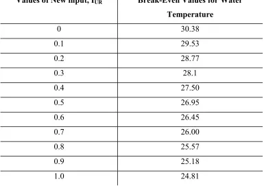
Table 4-8. Range of the break-even combinations for water temperature and IUR... 79

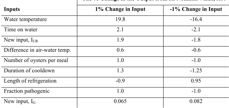
Table 4-9. Results of differential sensitivity analysis for 1% change in the nominal values of inputs. ... 82

Table 4-10. Percent change in the output from its nominal value for ± 1% and ± 5% change in the inputs... 83

Table 4-11. Normalized regression coefficients calculated using @RISK and SAS. ... 86

Table 4-12. Steps of the stepwise regression analysis using SAS... 87

Table 4-13. Steps of the stepwise regression analysis using SAS for rank ordered data. ... 89

Table 4-14. Comparison of sensitivities in terms of regression coefficients and ranking of inputs for original data and rank ordered data. ... 89

Table 4-15. Instability in the results of linear regression analysis for two different samples using @RISK to demonstrate the effect of random sampling error. ... 90

Table 4-16. Correlation coefficient matrix for all inputs... 91

Table 4-17. Instability in the results of rank regression analysis for two different samples to demonstrate the effect of random sampling error. ... 92

Table 4-18. Sensitivities and ranking of individual inputs based on F values for the inputs. ... 94

Table 4-19. Sensitivities and ranking of interaction terms based on F values. ... 94

(14)

Table 4-21. R2 values for different terms in the RS model... 98

Table 4-22. The result of F test to evaluate the fit of the RS to the simulated data set... 99

Table 4-23. Range and nominal values of inputs used in the RS for NRSA. ... 101

Table 4-24. The results of NRSA using the RS and the actual Vp model. ... 101

Table 4-25. Comparison of the original and the alternative distribution for time on water. ... 105

Table 4-26. Comparison of the original and the alternative distribution for the number of oysters. ... 105

Table 4-27. Comparison of the original and the alternative distribution for duration of cooldown... 106

Table 4-28. Comparison of the original and the alternative distribution for refrigeration length. ... 106

Table 4-29. Comparison of the output, probability of illness, for modified Vp model in Simlab with alternative distributions and modified Vp model in EXCEL. ... 110

Table 4-30. First-order and total-order FAST indices from Simlab and normalized FAST indices for the output, probability of illness. ... 111

Table 4-31. Comparison of step R2 values from stepwise regression analysis and normalized total order FAST indices... 113

Table 4-32. Calculation of MII for the Input: Water Temperature ... 116

Table 4-33. Mutual information indices and sensitivity indices for the inputs... 119

Table 4-34. Comparison of conditional probabilities and sensitivity indices for three different simulations for the input, water temperature. ... 121

Table 5-1. Comparison of Ranking of Inputs According to Sensitivity Analysis Methods ... 132

Table 5-2. Overview of Comparison of the Methods ... 141

Table E-1. Calculation of MII for time on water... 180

Table E-2. Calculation of MII for IUR... 181

Table E-3. Calculation of MII for difference in air and water temperature. ... 182

(15)

Table E-5. Calculation of MII for duration of cooldown. ... 184

Table E-6. Calculation of MII for length of refrigeration. ... 185

Table E-7. Calculation of MII for fraction of pathogenic Vp. ... 186

(16)

LIST OF FIGURES

Figure 2-1. Example of a decision tree model and representation of the utility

of outcomes... 12

Figure 2-2. Example of a probability density function... 15

Figure 2-3. Example of a cumulative distribution function. ... 16

Figure 3-1. Example of chart for representing difference in log odds ratio. ... 23

Figure 3-2. Example of break-even analysis. ... 25

Figure 3-3. Three-dimensional surface representing conditional confidence analysis. ... 43

Figure 3-4. Change in the median of the output for different values of the input… ... 44

Figure 3-5. PDF of the output for a specific value of the input... 44

Figure 3-6. Distribution for the confidence in the decisions. ... 44

Figure 3-7. Example of a pattern for a scatter plot... 46

Figure 4-1. Schematic depiction of the harvest module of the Vp model... 52

Figure 4-2. Schematic depiction of the post-harvest module of the Vp model... 54

Figure 4-3. CDF of the empirical distribution for the number of oysters consumed per serving. ... 55

Figure 4-4. Schematic depiction of public health module of the Vp model... 56

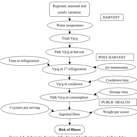
Figure 4-5. Schematic diagram of the Vp model with integration of all modules... 58

Figure 4-6. Schematic representation of conditional sensitivity analysis for an intermediate variable, air temperature. ... 66

Figure 4-7. Example of linear model response for the input, fraction of pathogenic Vp... 70

Figure 4-8. Example of nonlinear model response for the new input, IUR... 70

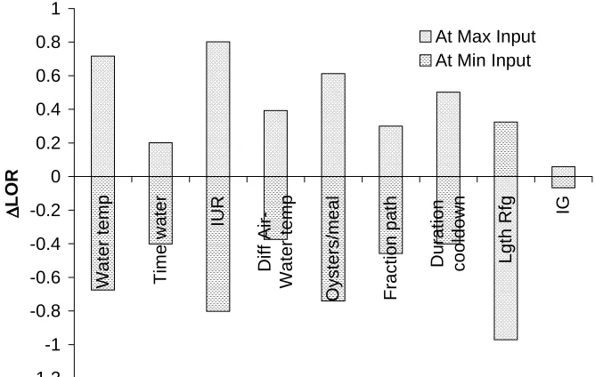
Figure 4-9. Graph of ∆LOR at minimum and maximum input values, and combined ∆LOR ... 74

(17)

Figure 4-11. Linear variation in the probability of illness versus nonlinear

variation in LOR for the number of oysters per meal... 76 Figure 4-12. Linear variation in the probability of illness versus nonlinear

variation in LOR for length of refrigeration. ... 77 Figure 4-13. Break-even line between water temperature and grams of oysters

consumed to decide whether or not the risk is acceptable... 78 Figure 4-14. Parity plot for the probability of illness from the RS versus the

probability of illness from the original model. ... 99 Figure 4-15. The response surface for probability of illness versus IUR and the

number of oysters per meal... 100 Figure 4-16. Comparison of CDFs of original and alternative distribution for

time on water. ... 106 Figure 4-17. Comparison of CDFs of original and alternative distribution for

oysters per meal. ... 107 Figure 4-18. Comparison of CDFs of original and alternative distribution for

duration of cooldown... 107 Figure 4-19. Comparison of CDFs of original and alternative distribution for

length of refrigeration. ... 108 Figure 4-20. Comparison of CDFs for the probability of illness calculated

using the modified Vp model in EXCEL (case 1) and the Vp

model in Simlab (case2). ... 110 Figure 4-21. Histogram for water temperature used to estimate the probabilities

of input values... 117 Figure 4-22. Conditional confidence plot (CDF) of the output for the input:

water temperature. ... 119 Figure 4-23. Scatter plot of probability of illness versus water temperature. ... 122 Figure 4-24. Scatter plots of probability of illness versus water temperature for

different ranges of the probability of illness... 123 Figure 4-25. Log-linear scatter plot of log of probability of illness versus water

(18)

Figure B-1. Variation in the probability of illness versus variation in LOR for

water temperature. ... 164

Figure B-2. Variation in the probability of illness versus variation in LOR for time on water. ... 164

Figure B-3. Variation in the probability of illness versus variation in LOR for IUR…… ... 165

Figure B-4. Variation in the probability of illness versus variation in LOR for difference in air and water temperature. ... 165

Figure B-5. Variation in the probability of illness versus variation in LOR for the number of oysters per meal... 166

Figure B-6. Variation in the probability of illness versus variation in LOR for duration of cooldown... 166

Figure B-7. Variation in the probability of illness versus variation in LOR for length of refrigeration. ... 167

Figure B-8. Variation in the probability of illness versus variation in LOR for pathogenic fraction of Vp. ... 167

Figure B-9. Variation in the probability of illness versus variation in LOR for IG……. ... 168

Figure E-1. Overall Confidence on the output... 176

Figure E-2. Conditional confidence plot for water temperature. ... 176

Figure E-3. Conditional confidence plot for time on water. ... 177

Figure E-4. Conditional confidence plot for unrefrigerated time. ... 177

Figure E-5. Conditional confidence plot for air temperature... 177

Figure E-6. Conditional confidence plot for oysters consumed per meal... 178

Figure E-7. Conditional confidence plot for duration of cooldown... 178

Figure E-8. Conditional confidence plot for length of refrigeration... 178

Figure E-9. Conditional confidence plot for fraction of pathogenic Vp... 179

Figure E-10. Conditional confidence plot for grams of oysters consumed. ... 179

Figure F-1. Scatter plot of probability of illness versus time on water. ... 188

(19)

Figure F-3. Log-linear scatter plot for time on water. ... 189 Figure F-4. Scatter plot of probability of illness versus IUR. ... 189 Figure F-5. Scatter plots of probability of illness versus IUR for different

ranges of IUR... 190 Figure F-6. Scatter plot of probability of illness versus IUR. ... 190 Figure F-7. Scatter plot of probability of illness versus difference in air and

water temperature. ... 191 Figure F-8. Scatter plots of probability of illness versus difference in air and

water temperature for different ranges of difference in air and

water temperature. ... 191 Figure F-9. Log-linear scatter plot for difference in air and water temperature... 192 Figure F-10. Scatter plot of probability of illness versus the number of oysters

per meal. ... 192 Figure F-11. Scatter plots of probability of illness versus the number of oysters

per meal for different ranges of the number of oysters per meal... 193 Figure F-12. Log-linear scatter plot for the number of oysters per meal. ... 193 Figure F-13. Scatter plot of probability of illness versus duration of cooldown... 194 Figure F-14. Scatter plots of probability of illness versus duration of cooldown

for different ranges of duration of cooldown... 194 Figure F-15. Log-linear scatter plot for duration of cooldown... 195 Figure F-16. Scatter plot of probability of illness versus length of refrigeration. ... 195 Figure F-17. Scatter plots of probability of illness versus length of refrigeration

for different ranges of length of refrigeration... 196 Figure F-18. Log-linear scatter plot for length of refrigeration... 196 Figure F-19. Scatter plot of probability of illness versus fraction of pathogenic

Vp…… ... 197 Figure F-20. Scatter plots of probability of illness versus fraction of pathogenic

(20)

Figure F-23. Scatter plots of probability of illness versus IG for different ranges

(21)

1.0 INTRODUCTION.

Concern for the safety of the food supply is motivated by recognition of the significant impact of microbial food borne diseases in terms of human suffering and economic costs to the society and industry, and an increasing global food trade (Lammerding, 1997). Mead et al. (1999) have reported that food borne disease results in 76 million human illnesses in the United States each year, including 325,000 hospitalizations and 5,200 deaths. ERS (2001) estimated the cost of food borne disease to be $6.9 billion annually. Food safety is gaining increased attention because of several trends. New food borne pathogens are emerging (Buchanan, 1996). Larger batch production, distribution, and longer shelflife of food products contribute to broader exposure to contaminating events. The proportion of food consumed that is supplied by food services is growing and this reduces consumer control over food handling and processing. Demand for safer food is growing as consumers are becoming more affluent, live longer, and are better informed about diet (McKone, 1996). International trade in food also can introduce new sources of risks to food safety, such as cattle or meat acquiring infection overseas.

Food safety regulatory agencies are taking a new approach to ensuring the safety of food supply based upon the Hazard Analysis Critical Control Points (HACCP) system (FSIS, 1999). One step in the HACCP system is to determine critical control points (CCP) where risk

management efforts can be focused. Food safety depends on many factors, such as composition and preparation of the product, process hygiene, and storage and distribution conditions

(Zwietering and Gerwen, 2000). Given data gaps and the complexity and dynamic nature of the food processing, transportation, storage, distribution, and preparation system, determining which of the many nodes in the farm-to-table pathway constitute CCPs and represents a substantial analytical challenge (Rose, 1993; Buchanan et al., 2000).

(22)

analysis can be used as an aid in identifying the importance of uncertainties in the model for the purpose of prioritizing additional data collection or research (Cullen and Frey, 1999).

Furthermore, sensitivity analysis can play an important role in model verification and validation throughout the course of model development and refinement (e.g., Kleijnen, 1995; Kleijnen and Sargent, 2000; and Fraedrich and Goldberg, 2000). Sensitivity analysis also can be used to provide insight into the robustness of model results when making decisions (e.g., Phillips et al., 2000; Ward and Carpenter 1996; Limat et al.,2000; Manheim 1998; and Saltelli et al., 2000).

Sensitivity analysis methods have been applied and additional knowledge about the sensitivity analysis is emerging from theses applications in various fields including complex engineering systems, economics, physics, social sciences, medical decision making, and others (e.g., Oh and Yang, 2000; Baniotopoulos, 1991; Helton and Breeding, 1993; Cheng, 1991; Beck et al., 1997; Agro et al., 1997; Kewley et al., 2000; Merz et al., 1992).

1.1 Objectives and Motivation.

The objectives of this paper are to identify, review, and evaluate sensitivity analysis methods for applicability to risk assessment models typical of those used, or expected to be used, in the near future for food safety risk assessment. As the key objective in this task is to benefit from knowledge across many disciplines, the literature review extends well beyond food safety to include many other fields. This objective serves as an aid in identifying potential CCPs along the farm-to-table continuum, to inform decisions about food safety research and data acquisition priorities, and to contribute to the development of sound food safety regulations. The identified methods will be applied to a typical food safety risk assessment model so that issues related to the application of the sensitivity analysis methods can be identified.

1.2 Importance of Risk Assessment in Food safety.

The objective of the risk assessment is to answer three risk questions (Kaplan and Garrick, 1981):

• What can go wrong?

(23)

• What would be the consequences if it did go wrong?

Risk assessment provides structured information that allows decision makers to identify interventions that can lead to public health improvement or to avoid future problems.

The HACCP system is used to prevent hazards associated with foods. The best information of the risk from such hazards that industry may have today is qualitative, such as whether a hazard presents a high, medium, or low risk (WHO, 2001). The outcome of a

HACCP-based system should be improved food safety assurance, measured by reduction in risk to the consumer and not merely a reduction in the level of a hazard in a food (Hathaway, 1995). Risk assessment can be used to determine which hazards are essential to control, to reduce, or to eliminate (Buchanan, 1995; Hathaway, 1995; and Notermans et al., 1995). Therefore, risk assessment can help in developing more effective HACCP plans.

Risk assessments can play an important role in international trade by ensuring that countries establish food safety requirements that are scientifically sound and by providing a means for determining whether different standards provide equivalent levels of public health protection (WHO, 2001). Without a systematic risk assessment, countries may set requirements that are not related to food safety and can create artificial barriers to trade.

1.3 Risk Assessment Framework.

As defined by the Codex Alimentarius Commission (CAC), risk assessment is a scientifically based process consisting of four main steps: hazard identification, hazard characterization, exposure assessment, and risk characterization (FAO, 2001). These steps are similar to those defined in the risk analysis framework of the National Academy of Science (NRC, 1983). Each of these four steps is described briefly according to CAC definitions.

(24)

• Hazard Characterization. Hazard characterization is the qualitative and/or quantitative evaluation of the nature of the adverse health effects associated with biological, chemical, and physical agents that may be present in food. Hazard characterization may or may not include dose-response assessment.

• Exposure Assessment. Exposure assessment is the qualitative and/or quantitative evaluation of the likely intake of biological, chemical, and physical agents via food as well as exposures via other sources, if relevant.

• Risk Characterization. Risk characterization involves qualitative and/or quantitative estimation, including attendant uncertainties, of the probability of occurrence and severity of known or potential adverse health effects in a given population based on hazard

identification, hazard characterization, and exposure assessment.

1.4 Important Issues in Food safety risk modeling.

There are many important issues in modeling as applied to risk assessment that motivate the need for sensitivity analysis and that illustrate the key challenges that sensitivity analysis faces or that can be addressed by sensitivity analysis. Cullen and Frey (1999) discuss issues such as purpose of models, model extrapolation, inappropriate application of models, complex

models, and model verification and validation. 1.4.1 Purpose of the Model.

The purpose of a model is to represent as accurately as necessary a system of interest. A system is typically comprised of many components. All modeling involves decisions regarding aggregation and exclusion (Cullen and Frey, 1999). Aggregation refers to simplified

representation of complex real world systems. Exclusion refers to a decision to omit any portions that are judged not to be important with respect to modeling objectives.

(25)

mind. For example, three different objectives are addressed by screening analysis models, research models, and assessment/decision making models, respectively.

Screening analysis is usually based on simple models that are not likely to underestimate the risk. The purpose of this analysis is usually to help the decision maker with routine

regulatory decisions. Screening methods are intended to help identify exposure pathways that are not important and to do so with a great deal of confidence. Screening methods cannot be used to prove that a particular exposure pathway is important. Rather, they can identify exposure pathways that should receive priority for further evaluation and analysis. Because screening models are conservative, they are designed to provide some "false positives." This means that they will often provide results indicating that a exposure pathway is of concern, but later analysis with more refined assumptions or models may reveal less of a problem. A key advantage of screening models is that they are often easier to use than more refined models. Screening models typically have fewer input data requirements and involve less complex calculations.

Research models are intended to improve understanding of the function and structure of real systems. They allow a researcher to explore possible and plausible functional relationships and may involve many detailed mechanisms. Research models may be complicated and may not be aimed at any particular risk management end point. As such, they may have large input data requirements, be difficult to execute, and provide output not directly relevant to a specific risk management objective. However, such models can be very helpful in improving fundamental insights regarding risk processes and in learning lessons useful for further model development.

(26)

Sensitivity analysis is important for all three types of models. In the context of this discussion, refined risk models are perhaps the most relevant. Sensitivity analysis can be used to evaluate how robust risk estimates and management strategies are to model input assumptions and can aid in identifying data collection and research needs.

1.4.2 Complex Models.

A model can be small yet complex. Model size should not be confused with model complexity. Complex systems are often hierarchies, which can be described in terms of the "span" of each level in the hierarchy and the number of levels (Reed and Afjeh, 2000; Simon, 1996).

Food safety risk models typically: (1) are nonlinear; (2) contain discrete inputs; (3) contain thresholds; (4) contain multiple pathways; and (5) are modular. The nonlinear and threshold features imply that interactions are important. For example, if temperature is low enough, then there may be no microbial growth, but once temperature exceeds a threshold, then the model may predict a nonlinear response that depends on several model inputs. The

modularity feature means that computations may take place in separate modules of the models, and only a selected set of aggregated results may be passed from one module to another. 1.4.3 Model Verification and Validation.

Model verification is a process of making sure that the model is doing what it is intended to do. Sensitivity analysis can be helpful in verification. If a model responds in an unacceptable way to changes in one or more inputs, then troubleshooting efforts can be focused to identify the source of the problem.

Model validation ideally involves comparison of model results to independent

(27)

(Hoffman and Miller, 1983). Cullen and Frey (1999) discuss partial validation of a model when observational data are available for only a part of the modeling domain.

Sensitivity analysis can be used to help develop a "comfort level" with a particular model. If the model response is reasonable from an intuitive or theoretical perspective, then the model users may have some comfort with the qualitative behavior of the model even if the quantitative precision or accuracy is unknown.

1.4.4 Model Extrapolation.

A model is applicable within the specific set of inputs and outputs associated with the data used for calibration or validation of the model. Model extrapolation involves making predictions for a situation beyond the range of calibration or validation of the model. For example, Guassian-plume-based air dispersion models are applicable only for distances up to about 20 km or 50 km from the emission source. The model should not be used to characterize long-range transport over hundreds of kilometers.

Empirical models such as ones developed from regression analysis are generally based on a specific data set. Regression analysis may be based on arbitrary functions to approximate relationships between the data. However, there may not be any theoretical basis for the functional relationship selected. In such a situation, if the inputs used are outside the original data set from which the regression model was developed then the output may not valid. There are two types of extrapolations. Explicit extrapolation involves making predictions for values of inputs outside the range of values for which the model was calibrated or validated. Hidden extrapolation involves specifying combinations of inputs for which validation has not been done, even though each of the input values fall within the range of values that have been tested. If the functional form of the relationship between the output and the inputs of the model is based on sound theoretical assumptions, then the model may perform reasonably well when extrapolated. Sensitivity analysis can be used to reveal how the model performs when the model is

(28)

1.5 Sensitivity Analysis Methods.

Sensitivity analysis methods can be classified in a variety of ways. In this report, they are classified as: (1) mathematical; (2) statistical; and (3) graphical. Other classifications focus on the capability, rather than the methodology, of a specific technique (e.g.,Saltelli et al., 2000). Classification schemes aid in understanding the applicability of a specific method to a particular model and analysis objective. Here, the focus is on sensitivity analysis techniques applied in addition to the fundamental modeling technique. For example, an analyst may perform a deterministic analysis, in which case a mathematical method, such as nominal range sensitivity can be employed to evaluate sensitivity. Alternatively, an analyst may perform a probabilistic analysis, using either frequentist or Bayesian frameworks, in which case statistical-based sensitivity analysis methods can be used (e.g., Cullen and Frey, 1999; Box and Tiao, 1992; Saltelli et al., 2000; Weiss, 1996).

1.5.1 Mathematical Methods for Sensitivity Analysis.

Mathematical methods assess sensitivity of a model output to the range of variation of an input. These methods typically involve calculating the output for a few values of an input that represent the possible range of the input (e.g., Salehi et al., 2000). These methods do not address the variance in the output due to the variance in the inputs, but they can assess the impact of range of variation in the input values on the output (Morgan and Henrion, 1990). In some cases, mathematical methods can be helpful in screening the most important inputs (e.g., Brun et al., 2001). These methods also can be used for verification and validation (e.g., Wotawa et al., 1997) and to identify inputs that require further data acquisition or research (e.g., Ariens et al., 2000). Mathematical methods evaluated here include nominal range sensitivity analysis, break-even analysis, difference in log odds ratio, and automatic differentiation.

1.5.2 Statistical Methods for Sensitivity Analysis.

(29)

varied at a time. Statistical methods allow one to identify the effect of interactions among multiple inputs.

The range and relative likelihood of inputs can be propagated using a variety of techniques such as Monte Carlo simulation, Latin hypercube sampling, and other methods. Sensitivity of the model results to individual inputs or groups of inputs can be evaluated by variety of techniques (Cullen and Frey, 1999). Greene and Ernhart (1993), Fontaine and Jacomino (1997), and Andersson et al. (2000) give examples of the application of statistical methods. The statistical methods evaluated here include regression analysis, analysis of variance, response surface methods, Fourier amplitude sensitivity test, and mutual information index.

1.5.3 Graphical Methods for Sensitivity Analysis.

Graphical methods give representation of sensitivity in the form of graphs, charts, or surfaces. Generally, graphical methods are used to give visual indication of how an output is affected by variation in inputs (e.g., Geldermann and Rentz, 2001). Graphical methods can be used as a screening method before further analysis of a model or to represent complex

dependencies between inputs and outputs (e.g., McCamly and Rudel, 1995). Graphical methods can be used to complement the results of mathematical and statistical methods for better

representation (e.g., Stiber et al., 1999; Critchfield and Willard, 1986). 1.5.4 Bayesian Sensitivity Analysis Methods.

(30)

analysis. Saltelli et al. (2000) have described a few approaches for evaluating sensitivity to the prior. More complex analyses to evaluate sensitivity to the prior and to the utility can be based on the theory of maximin solutions as described by Saltelli et al. (2000).

1.6 Application of the Methods on a Food Safety Risk Assessment Model.

Review of the sensitivity analysis methods can help one understand the potential

strengths and limitation of each method. However, the specific issues regarding the applicability of the sensitivity analysis methods to food safety risk assessment models can be only identified by applying the methods to a typical food safety risk model. Section 4 will deal with the application of the methods in more detail.

1.7 Organization of the Report.

Section 2 provides a glossary of terms used in the report. Section 3 identifies, describes, and evaluates ten selected sensitivity analysis methods. Section 4 illustrates case study

(31)

2.0 GLOCERY OF TERMS USED IN THE REPORT.

This section describes important terms used in the report. Concepts regarding a few important terms such as "decision analysis," "probability density function," "cumulative density function," and "simulation" are also provided in brief.

2.1 Input/Output Variables and Model Domain Parameters.

Inputs are used by analysts to feed information into a model. Inputs are typically controlled by the user. Inputs may have a single value, or they may be variable, uncertain or both (Bogen, 1990). Outputs are information provided by use of the model. These variables are typically final outcomes of a model, which are then used in decision making. Model domain parameters specify the domain or scope of the system being modeled, generally by specifying the range and increments for index variables used to identify a location or cell in the spatial or

temporal domain of the model (Morgan and Henrion, 1990). Model domain parameters are associated with a model, but not directly with the phenomenon the model represents (Cullen and Frey, 1999). For example, the spatial or temporal grid size is a model domain parameter

introduced in numerical models. In models of the transport of atmospheric pollution, the spatial extent of the model may be controlled by domain parameters specifying the "ceiling height" and minimum and maximum longitude and latitude. Domain parameters may also be used to define baseline properties. For example, in performing generic analysis of the risks of alternative types of power plants, the analyst may arbitrarily select the size of the plants for modeling at 1000 MW for purpose of comparison. Model domain parameters are quantities that control precision of the representation and the computational complexity and hence, are important to consider in

uncertainty analysis (Morgan and Henrion, 1990).

2.2 Decision Analysis.

(32)

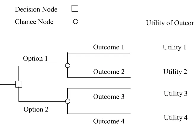
Figure 2-1. Example of a decision tree model and representation of the utility of outcomes.

of decision trees. For example, decision trees may be used to represent CCPs in a HACCP system (Lee and Hathaway, 1998). A primary analysis is needed to determine whether a decision node is critical. A decision tree consists of decision nodes and chance nodes as shown in Figure 1. Decision nodes indicate options available to the decision maker, whereas chance nodes indicates outcomes beyond the control of the decision maker that may result from a particular option (Brown, 1974). The outcome at any chance node can depend on outcomes at other chance and decision nodes. The output of the model can be several outcomes that can result depending on outcomes at previous nodes in the model. Decision analysis can be coupled with probabilistic analysis for decision making under uncertainty (Harwood, 2000).

In decision tree models, each of the final outcomes have some relative importance to the decision maker. This importance is accounted for by use of a value, known as utility of that outcome to the decision maker (Brown, 1974). The utility of an outcome is proportional to importance of that outcome. The utility of an outcome can be a negative value indicating the importance of avoiding that outcome. The value of the utility is subjective to the decision maker. In Figure 1, each of the four outcomes will have a utility to a decision maker. More information on decision analysis is given by Brown (1974), and Watson and Buede (1987).

Decision Node Chance Node

Outcome 1

Outcome 2

Outcome 3

Outcome 4 Option 2

Option 1

Utility 1

Utility 2

Utility 3

(33)

2.3 Deterministic Analysis.

In deterministic analysis (or models), analysts perform calculations using point estimates representing inputs, giving point estimates for the outputs of a model. The purpose of

deterministic models can be to provide decision makers with a best estimate of the risk (Cullen and Frey, 1999). In deterministic analysis, quantitative measures of accuracy and precision of model predictions are not developed, because no information on model or input uncertainty is accounted for quantitatively (Cullen and Frey, 1999). Deterministic analysis can be used in screening analysis. In the case of screening analysis, the values of model inputs may be selected to lead to a conservative result for the model outputs. "Deterministic" also refers to the notion that for a given set of input values, there is only one unique response of the system. Most models used in risk assessment are deterministic in the sense that there is an underlying

hypothesis of a cause and effect relationship. However, deterministic models may be exercised to take either uncertainty and/or variability into account, as discussed in later sections.

2.4 Probabilistic Analysis.

Probabilistic analysis can be used with deterministic models to propagate uncertainties and/or variability in inputs to estimate uncertainty and/or variability in model outputs.

(34)

2.4.1 Uncertainty.

Uncertainty may be thought of as a measure of the incompleteness of one's knowledge or information about an unknown quantity whose true value could be established if a perfect

measuring device were available (Cullen and Frey, 1999). Random and systematic measurement errors and inability of models to truly describe a physical, chemical, or biological system are sources of uncertainty. Uncertainty may be reduced by additional study or measurement. 2.4.2 Variability.

Variability refers to temporal, spatial, or interindividual differences in the value of an input (Cullen and Frey, 1999). For example, the consumption rate of specific dietary items for individuals changes over time, different regions, and different individuals. Variability cannot be reduced by means of additional study or measurements.

To explain variability and uncertainty, consider an example of disease prevalence. At any point in time, prevalence is fixed but unknown within a population. Therefore, prevalence is an uncertain quantity. However, management interventions, such as immunization can shift the position and attenuate the spread in prevalence. Therefore, prevalence can be a variable quantity dependent on the management interventions.

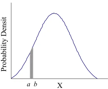
2.4.3 Probability Density Function.

A probability distribution model is typically represented mathematically as a probability density function (PDF) or a cumulative distribution function (CDF). The probability that a continuous random variable X is within a specified range is determined by the PDF of X. The PDF is a graphical means of representing the relative likelihood with which values of an input may be obtained (Cullen and Frey, 1999). The PDF can be denoted f(x) and is defined as: f(x)≥

(35)

0 0.2 0.4 0.6 0.8 1

X

Cumulative Probabilit

y

X

Probability Densi

t

to 1. For continuous distributions, the units of probability density are the inverse of the units of the random variable, X.

a b Figure 2-2. Example of a probability density function.

2.4.4 Cumulative Distribution function.

A probability distribution also can be represented as a CDF. The CDF is obtained by integrating the PDF. The y-axis of the CDF is scaled in percentiles, and the x-axis shows the value of the variable X associated with each percentile. The CDF shows fractions of all possible values of x which are less than or equal to a given value of x (Cullen and Frey, 1999). The CDF is usually specified as F(x) = Pr(X≤x), where F(x) is the integral of f(x) up to the value of x. F(x) is bounded by zero and one. The cumulative probability that X is less than or equal to a is value of F(x) corresponding to a, as shown in Figure 3. In the example shown, the cumulative probability of a is 0.3, meaning that the value a occurs at the 30th percentile of the distribution.

(36)

Figure 2-3. Example of a cumulative distribution function. 2.4.5 Simulation.

Probabilistic analysis typically requires simulation to propagate variability and uncertainty in inputs through the model to estimate the corresponding distribution of model outputs. A simulation involves propagating random values of an input according to its probability distribution, through a model. A single run in a simulation is referred to as one realization and values of inputs used are referred to as samples. Generally two types of probabilistic simulation techniques are commonly used: Monte Carlo simulation and Latin hypercube sampling (LHS). These two methods are described in brief. More information is given by Cullen and Frey (1999).

Conceptually Monte Carlo simulation involves randomly generating a uniformly

distributed number u between 0 and 1, which is denoted as u ~ U(0,1). The inverse CDF, F-1(u), is calculated for each value of u. F-1(u) will give a unique value of an input variable, which is based on the distribution of the input. Given a uniformly distributed random variable, several methods exist from which to simulate random variables that are described by other probability distributions (e.g., normal, lognormal, Weibull, and others). These methods include the inverse transform, composition, and function of random variables (e.g., Ang and Tang, 1984). The unique simulated input value is then used in one realization of the simulation. The above mentioned process is repeated for all the values of u generated randomly.

Methods called restricted pairing techniques in conjunction with Monte Carlo can

simulate correlation or dependence among inputs. Cullen and Frey (1999) have more discussion on simulating correlated inputs.

(37)

LHS is not a truly random process because of the restraint of dividing the sample space into N intervals. Because the samples used to define probability distributions for an input are selected from intervals that are evenly spaced over the range of probable values of the input, the number of samples needed to adequately represent the CDF of a variable is less than that for Monte Carlo sampling. For further discussion on the LHS method refer to Cullen and Frey (1999).

2.5 Dichotomous Output and Dichotomous Model.

A model that gives a dichotomous output is referred to as a dichotomous model. A dichotomous output is one that has only two possible results. Usually, these results are qualitative such as risk is acceptable or risk is unacceptable. Dichotomous models can be probabilistic. In the case of probabilistic models, a range of output values specifies an unique output. For example, for risk indicator values less than 10-6, the risk is acceptable or else the risk is unacceptable. Dichotomous models are often decision tree type models.

(38)

(39)

3.0 SENSITIVITY ANALYSIS METHODS.

This section identifies sensitivity analysis methods used across various disciplines. Reference materials, such as journals, reports, books, and the World Wide Web were collected from various fields including medical decision making, engineering, economics, health science, and food science. Methods that were applied on models comparable to risk assessment models were identified for evaluation. The methods and specific applications of each method are demonstrated. Strengths and limitations of the methods are noted in brief.

3.1 Nominal Range Sensitivity.

Nominal range sensitivity method is also known as local sensitivity analysis or threshold analysis (Cullen and Frey 1999; Critchfield and Willard, 1986). This method is applicable to deterministic models. It is usually not used for probabilistic analysis. One use of nominal sensitivity analysis is as a screening analysis to identify the most important inputs to propagate through a model in a probabilistic framework (Cullen and Frey, 1999). Nominal range

sensitivity can be used to prioritize data collection needs as demonstrated by Salehi et al. (2000). 3.1.1 Description.

Nominal range sensitivity analysis evaluates the effect on model outputs exerted by individually varying only one of the model inputs across its entire range of plausible values, while holding all other inputs at their nominal or base-case values (Cullen and Frey, 1999). The difference in the model output due to the change in the input variable is referred to as the

sensitivity or swing weightof the model to that particular input variable (Morgan and Henrion, 1990). The sensitivity also can be represented as a positive or negative percentage change compared to the nominal solution. The sensitivity analysis can be repeated for any number of individual model inputs.

(40)

given input may depend on interactions with other inputs, which are not considered. Thus, the results of nominal range sensitivity are potentially misleading for nonlinear models.

3.1.2 Application.

Two examples of the use of nominal range sensitivity analysis are given here. In the first, nominal range sensitivity was applied as described here to an exposure assessment problem for flounder in a contaminated harbor (Dakins et al., 1994). The selection of inputs evaluated in the sensitivity analysis, and the range of values assigned to those inputs, was based upon literature review. The absolute different in burden of PCB in flounder was the key measure of sensitivity. An absolute difference of less than 0.5 µg PCB per gram of body weight was considered to be non-sensitive.

In the second example, a conditional nominal range sensitivity analysis was performed (Sinicio et al., 1997). The objective of the analysis was to determine the allowable safe storage time for grain wheat as a function of grain moisture content and temperature conditioned upon key assumptions of a ventilation system. The intent was to recommend airflow rates and fan control strategies to properly aerate the stored grains. The sensitivity analysis was conditioned on two different assumptions regarding the airflow rate and two different assumptions regarding the air temperature rise in the fan, leading to four different cases. For each case, three specific inputs were each varied over a nominal range, and the impact on the key model output, allowable storage time elapsed, was evaluated. Specific heat of the wheat was observed to be the most sensitive input for each of the four cases.

3.1.3 Advantages.

(41)

3.1.4 Disadvantages.

Nominal sensitivity analysis addresses only a potentially small portion of the possible space of input values, because interactions among inputs are difficult to capture (Cullen and Frey 1999). Conditional sensitivity analysis may be used to account for correlation between inputs or nonlinear interactions in model response, but it has limitations because of the combinational explosion of possible cases. Potentially important combined effects on the decision (or output) due to small changes in a few or all inputs together are not shown by nominal sensitivity analysis For other than linear models, it is not clear that nominal range sensitivity can provide a reliable rank ordering of key inputs.

3.2 Difference in Log-Odds Ratio (∆∆∆∆LOR).

The difference in the log odds ratio (∆LOR) method is a specific application of nominal range sensitivity methodology. The ∆LOR is used when the output is a probability. For

example, Song et al. (2000) used ∆LOR for identifying the most important inputs so that additional data collection and research can be prioritized.

3.2.1 Description.

The odds or odds ratio of an event is a ratio of the probability that the event occurs to the probability that the event does not occur (Walpole and Myers, 1993). If an event has a

probability of occurrence as P, then the odds ratio is P/(1-P). The log of the odds ratio or logit is just another convenient way of rescaling probabilities (Menard, 1995). Probabilities between 0 and 1 are equivalent to log odds between minus infinity and infinity and probability of 0.5 is equivalent to log odds of zero. Log odds are considered by some to be the preferred

transformation of probability because they are putatively easier to understand (Christensen, 1990). For example, if probability of an event is 0.8, then

odds (event occurs) = 0.8/(1-0.8) = 0.8/0.2 = 4,

odds (event doesn’t occur) = 0.2/(1-0.2) = 0.2/0.8 = 1/4 = 0.4, log odds (event occurs) = log(0.8 / 0.2) = log 4 = 0.6, and

(42)

In the above example, the odds of the event occurring and the odds of the event not occurring are not symmetric around the odds of 1, which are equivalent to a probability of 0.5. The odds of the event occurring have a higher magnitude than the odds of the event not

occurring. The log odds of the event occurring and the log odds of the event not occurring are symmetric around 0, which corresponds to a probability of 0.5. The magnitude of the log odds of the event occurring and the log odds of the event not occurring are the same. The minus sign represents that the event is not occurring. Therefore, unlike odds, log odds transform

probabilities on a linear scale and hence, are a more logical transformation of probability (Christensen, 1990).

The ∆LOR method is used to examine the change in the output as:

      −       = ∆ ) | Pr( ) | Pr( log ) | Pr( ) | Pr( log changes without event No changes without event input in changes with event No input in changes with event LOR .

If ∆LOR is positive, changes in one or more inputs enhance the probability of the specified event. If ∆LOR is negative, then the changes in the inputs cause a reduction in the probability of the event occurring or increase the probability of the event not occurring. The greater the magnitude of ∆LOR, the greater is the influence of the input (Stiber et al., 1999).

3.2.2 Application

(43)

is positive evidence of the degradation of TCE. From the sensitivity analysis, it appears that evidence regarding DCE is the most important determinant of anaerobic degradation of TCE, because changes in evidence for this particular input lead to the largest differences in the log-odds ratio.

Figure 3-1. Example of chart for representing difference in log odds ratio. (Source: Stiber et al., 1999)

The ∆LOR method is a useful measure of sensitivity when the model output is a probability (Menard, 1995).

The ∆LOR method can only be used when the output is in terms of probability (Menard, 1995). It suffers from other drawbacks similar to nominal range sensitivity analysis. For example, similar to nominal range sensitivity analysis, ∆LOR cannot account for nonlinear interactions between or among inputs. Similar to nominal range sensitivity analysis, the significance of differences among the sensitivities can be difficult to determine for nonlinear models and correlated inputs, making it potentially difficult to rank order key inputs.

- 1 - 0 .5 0 0 .5 1 1 .5 2

Log-odd Ratio

Terminal Electron Hydrogen

Redox Potential Dissolved Org. C BTEX TPH

Oxygen

Temperature pH

DCE

Vinyle Chloride

Ehene & Ethane Methane

(44)

3.3 Break-Even Analysis.

Break-even analysis is more of a concept than a specific method. Broadly speaking, the purpose of break-even analysis is to evaluate the robustness of a decision to changes in inputs (von Winterfeldt and Edwards, 1986).

Break-even analysis involves finding values of inputs that provide a model output for which a decision maker would be indifferent among the two or more risk management options. The combinations of values of inputs for which a decision maker is indifferent to the decision options are known as switchover or break-even values. Then, in order to assess the robustness of a choice between the options, one can evaluate whether the possible range of values of the model inputs corresponds with only one of the two choices (Morgan and Henrion, 1990). Indifference of a decision maker to the two choices is often represented by a break-even line or indifference curve such as an iso-risk curve. Ambiguity regarding selecting a particular choice exists if the uncertainty range associated with an output may correspond to either of the two or more possible choices. Different options that result in equivalent levels of risk reduction also can be identified so that a decision maker can evaluate these options. If there are more than two decision options, the analysis can get complex (von Winterfeldt and Edwards 1986).

Break-even analysis is often used in economics for purposes such as budget planning (Dillon, 1993). Break-even analysis has also found applications in several other fields such as health care (Boles and Fleming, 1996). Kottas and Lau (1978) describe the concept of stochastic break-even analysis. Starr and Tapiero (1975) explain the use of break-even analysis with consideration of risk.

(45)

and the probability of success of the operation that lead to a preference for medication, as in the upper left portion of the graph, or for the operation, as in the lower right portion of the graph. Along the indifference line, there is equal preference for both options. If the patient has a high utility for the outcome of the medication, and believes that the probability of success of the operation is low, then medication is clearly preferred. If the range of uncertainty in the

probability of success is large, and if the range of uncertainty encloses the indifference line, then it will be ambiguous as to what treatment option is preferred. In the former case, a decision can be made that is robust to uncertainty. In the latter case, more information is needed to reduce uncertainty in one or more of the inputs in order to make a decision with a high degree of confidence.

Figure 3-2. Example of break-even analysis. 3.3.3 Advantages.

The switchover or break-even point guides further modeling and elicitation. If the range of uncertainty regarding an input encloses the break-even point, then that input will be important in making a decision; that is, there will be uncertainty regarding which decision to take. In such a situation, further research can be directed so as to help the decision maker to narrow the range of uncertainty and make a decision with more confidence. On the other hand, if the uncertainty regarding an input does not enclose the break-even point then there will be high confidence regarding the decision.

-50 -30 -10 10 30 50 70 90

0 0.2 0.4 0.6 0.8 1

P of Success of Operation

Utility of Medication, M

Medication is favored

(46)

Break-even analysis is not a straightforward method to apply. Though it is a useful concept, its application is increasingly complex as the number of sensitive inputs increases (von Winterfeldt and Edwards, 1986). There also is not a clear ranking method to distinguish the relative importance of the sensitive inputs.

3.4 Automatic Differentiation Technique.

The automatic aifferentiation (AD) technique is an automated procedure for calculating local sensitivities for large models. In AD, a computer code automatically evaluates first-order partial derivatives of outputs with respect to small changes in the inputs. The values of partial derivatives are a measure of local sensitivity.

Most existing sensitivity analysis methods based upon differentiation, such as numerical differential methods, have one or more of the following limitations: inaccuracy in the results, high cost in human effort and time, and difficulty in mathematical formulation and computer program implementation (Hwang et al., 1997). To overcome these limitations, AD techniques were developed. AD is a technique to perform local sensitivity analysis and not a new method in itself. In AD the local sensitivity is calculated at one or more points in the parameter space of the model. At each point, the partial derivative of the model output with respect to a selected number of inputs is evaluated.

(47)

Automatic differentiation finds application in models that involve complex numerical differentiation calculations such as partial derivatives, integral equations, and mathematical series (Hwang et al., 1997). It is used in fields such as air quality (Carmichael et al., 1997), aerodynamics (Issac and Kapania, 1997), mechanical structures (Ozaki et al., 1995), and others. Christianson (1999) used AD for verification of part of a model.

As an example, Carmichael et al. (1997) applied ADIFOR to calculate the sensitivity of ambient air ozone concentration to air quality model inputs representing initial conditions, reaction rate constants, and others. For this purpose, dimensionless sensitivity coefficients were calculated based upon the numerical partial derivative of ozone concentration with respect to a selected input, divided by the ratio of the values of the concentration and the input:

Si,j =

                ∆ ∆ j i j i α C α C (3-1) where,

Si,j = Normalized local sensitivity coefficients for ith chemical specie and jth input;

∆Ci = The absolute change in the output concentration of ith chemical specie;

∆αj = The absolute change in the jth input;

αj = Values of model inputs; and

Ci = Concentration of a chemical specie i at a given time.

(48)

chemical specie is the summation of normalized local sensitivities at different time stages for that chemical specie.

AD techniques, such as ADIFOR can be applied without having detailed knowledge of the algorithm implemented in the model. ADIFOR does everything automatically once it is appended with the main code (Bischof et al., 1992). AD is superior to finite difference approximations of the derivatives because numerical values of the computed derivatives are more accurate and computational effort is significantly lower (Bischof et al., 1992). Hwang et al. (1997) observed CPU time saving of 57% by using AD for sensitivity analysis as compared to using a traditional method. If the model is constantly modified and improved, then ADIFOR provides a convenient tool to easily accommodate such necessary model changes, which can be very difficult to do in the case of other techniques (Carmichael et al., 1997).

The availability of AD technique may be limited to specific computer languages such as FORTRAN in the case of ADIFOR, requiring the user to provide FORTRAN code for the model. Because AD is a local technique, it suffers from the limitations of nominal range

sensitivity analysis. Furthermore, unlike nominal range sensitivity analysis, the possible range of values of the inputs is not considered. The accuracy for sensitivity results is conditioned upon the numerical method used in the AD software. Also, for nonlinear models, the significance of differences in sensitivity between inputs is difficult to determine, making the rank ordering of key inputs potentially difficult. This method cannot be used if partial derivatives cannot be evaluated locally.

3.5 Regression Analysis.