Improving Predictability of Simulation Models using Evolutionary Computation-Based Methods for Model Error Correction

(1)

ABSTRACT

ZECHMAN, EMILY MICHELLE. Improving Predictability of Simulation Models using Evolutionary Computation-Based Methods for Model Error Correction. (Under the direction of S. Ranji Ranjithan.)

Simulation models are important tools for managing water resources systems. An optimization method coupled with a simulation model can be used to identify effective decisions to efficiently manage a system. The value of a model in decision-making is degraded when that model is not able to accurately predict system response for new management decisions. Typically, calibration is used to improve the predictability of models to match more closely the system observations. Calibration is limited as it can only correct parameter error in a model. Models may also contain structural errors that arise from mis-specification of model equations. This research develops and presents a new model error correction procedure (MECP) to improve the predictive capabilities of a simulation model. MECP is able to simultaneously correct parameter error and structural error through the identification of suitable parameter values and a function to correct misspecifications in model equations. An evolutionary computation (EC)-based implementation of MECP builds upon and extends existing evolutionary algorithms to simultaneously conduct numeric and symbolic searches for the parameter values and the function, respectively. Non-uniqueness is an inherent issue in such system identification problems. One approach for addressing non-uniqueness is through the generation of a set of alternative solutions. EC-based techniques to generate alternative solutions for

(2)

(3)

IMPROVING PREDICTABILITY OF SIMULATION MODELS

USING EVOLUTIONARY COMPUTATION-BASED METHODS

FOR MODEL ERROR CORRECTION

by

EMILY MICHELLE ZECHMAN

A dissertation submitted to the Graduate Faculty of North Carolina State University

in partial fulfillment of the requirements for the Degree of

Doctor of Philosophy

CIVIL ENGINEERING

Raleigh

2005

APPROVED BY:

Dr. E. Downey Brill, Jr. Dr. G. Mahinthakumar

(4)

(5)

Biography

Emily Michelle Zechman was born on April 14, 1978, in Piqua, OH, the second of four girls to Thomas and Linda Zechman. She graduated from Piqua High School in 1996, and attended one year of college at Calvin College in Grand Rapids, MI, before transferring to the University of Kentucky, in Lexington, KY, where she graduated with her Bachelors of Science in Civil Engineering in 2000. She completed her Masters of Science in Civil Engineering under the direction of Dr. Lindell Ormsbee in 2001,

(6)

Acknowledgements

I would like to thank Dr. Ranji Ranjithan for all his labor to mentor me and teach me the skills of critical thinking and for always insisting on the very best effort I could give. I would like to thank Dr. Downey Brill for his continual encouragement and for asking practical and probing questions. He is a great teacher, who loves not to just teach, but for his students to truly learn. I would also like to express my gratitude to my

committee members, Drs. Jeff Joines and G. Mahinthakumar, for sharing their enthusiasm, knowledge, time and effort.

I would like to acknowledge my officemates for their research collaborations, thought-provoking discussions, feedback, support, and camaraderie, including Melinda King, Sunil Rao, Parthee Partheepan, Sivakumar Pabolu, Rachel Smith, Ken Harrison, Christos Anastasiou, Ozge Kaplan, Pam Schooler, Xin Jin, Baha Mirghani, Kaite Wang, Yong Jung, Matthew Clayton, Jessica Swanson, Li Liu, and Jihua Wang. I would like to acknowledge Jason Dorn, Michael Tryby, Dr. John Baugh, and Brett Humphreys for their help in the design of a computational framework for the implementation of this research.

My family has been a source of strength and encouragement to me. I would like to thank Kristin and Todd Baker, Abigail and Brett Humphreys, Sarah Jane and Kyle Magoteaux, Ethel and Bobby Dooney, Roberta and Dr. Detrick, and my parents, Thomas and Linda Zechman.

(7)

List of Figures

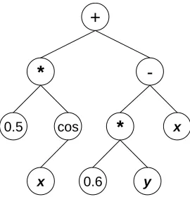
Figure 2.1 Calibration of a misspecified model by adjusting model parameter values... 7 Figure 2.2 Correction of a misspecified model using the model error correction procedure ... 9 Figure 2.3 Example tree representation of the equation 0.5cos(x) + 0.6y - x. ... 11 Figure 2.4 Correction of a misspecified model for dissolved oxygen deficit using

calibration to identify kd... 14

Figure 2.5 Identification of an empirical model as a function of inputs... 15 Figure 2.6 Correction of a misspecified model for dissolved oxygen deficit using MECP to identify kd and a function of model input (t, D0, and L0) and model output (D’). ... 16

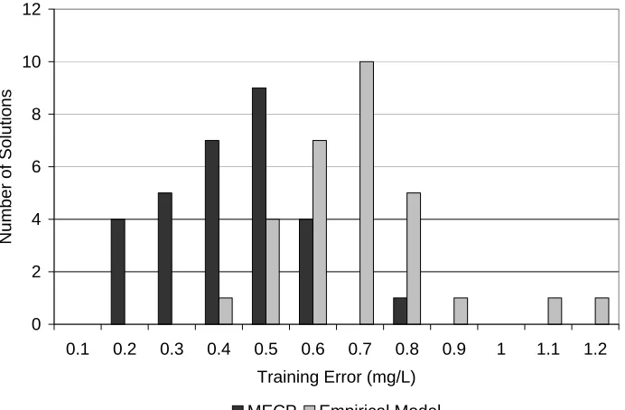
Figure 2.7 Training error for 30 random trials of MECP and GP-based search for

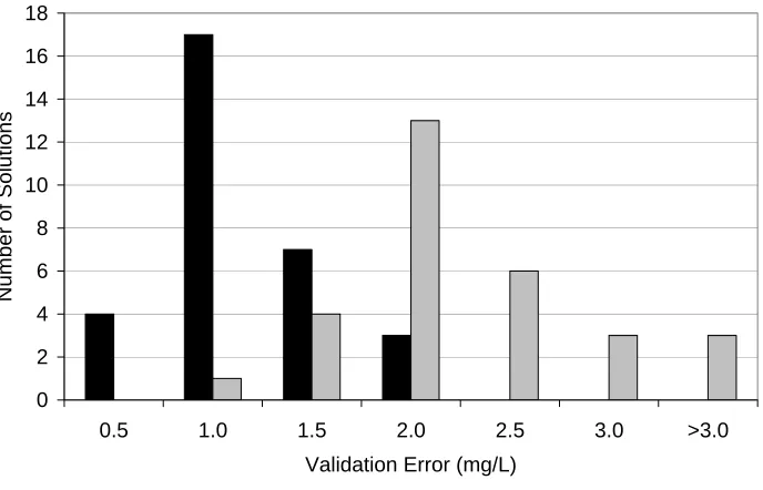
empirical model. ... 18 Figure 2.8 Validation error for 30 random trials of MECP and GP-based search for

empirical model. ... 19 Figure 2.9 Simulation capabilities of MECP-1, empirical model EMP-1, and calibrated model for a portion of the training data. ... 21 Figure 2.10 Predictive capabilities of MECP-1, empirical model EMP-1, and calibrated model for interpolated conditions. ... 22 Figure 2.11 Predictive capabilities of MECP-1, empirical model EMP-1, and calibrated model for extrapolated conditions. ... 23 Figure 3.1 Illustration of a two-objective space... 28 Figure 3.2 Objective and decision space for the one-dimensional test problem. ... 35 Figure 3.3 Objective landscape of the two-dimensional test function, with feasible

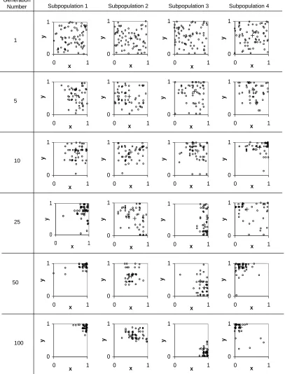
regions at F(x,y) > 4.528 projected onto the x-y plane. ... 38 Figure 3.4 Decision space at 12% relaxation for the two-dimensional test problem. ... 39 Figure 3.5 Distribution of the solutions in each subpopulation at the end of generations 1, 5, 10, 25, 50, and 100... 40 Figure 3.6 Comparison of performance of alternative solutions obtained using GAMGA, a niching with post screening procedure, and EAGA for the two-dimensional test

problem. ... 41 Figure 3.7 Airline network of eight cities... 42 Figure 3.8 Four alternative networks generated by EAGA. ... 46 Figure 3.9 Demand through each airport for four alternative solutions for a 10% cost relaxation... 47 Figure 3.10 Demand through each airport for four alternative solutions for a 5% cost relaxation... 48 Figure 4.1 The optimal solution (A) and the two most different alternative solutions (B and C) for the one-dimensional test problem... 60 Figure 4.2 Evolution of subpopulations over generations for the one-dimensional test problem ... 62 Figure 4.3 Schematic of wastewater treatment network options in DuPage County,

(10)

Figure 4.5 Comparison of flows at each plant for the three alternatives generated

simultaneously using EAGA... 71

Figure 4.6 Difference between pairs of networks for three sets of alternatives (Fig. 4.4).. ... 72

Figure 4.7 Variation of difference with number of alternative solutions generated... 74

Figure 4.8 Variation of difference metric with cost target for all solutions generated by simultaneous EAGA. ... 77

Figure 5.1 Two sample classifiers ... 90

Figure 5.2 Convergence of the four subpopulations... 96

Figure 5.3 Convergence of Average Difference ... 97

Figure 5.4 Average and range of prediction accuracy (% of correct hits) based on training dataset for 20 random trials... 98

Figure 5.5 Average and range of prediction accuracy (% of correct hits) based on validation dataset for 20 random trials... 98

Figure 5.6 Tree representation of a typical set of four classifiers found by MCCP ... 99

Figure 6.1 The configuration of the example groundwater field. The box in the lower left-hand corner represents the pollutant source, spheres represent monitoring locations. ... 110

Figure 6.2 Plan view of groundwater field with numbered monitoring locations for training data. ... 111

Figure 6.3 Concentration profile at Monitoring Well T1. ... 111

Figure 6.4 Plan view of groundwater field with numbered monitoring locations for validation and interpolation data... 112

Figure 6.5 Calibration of misspecified groundwater model to identify the dispersivity (α and the hydraulic conductivity field (k-field)... 115

Figure 6.6 Correction of a misspecified groundwater model using MECP to identify the dispersivity (α), the hydraulic conductivity field (k-field), and an error correction component as a function of model input (x, y, and t) and model output (C’). ... 116

Figure 6.7 Two example solutions for the correction of the misspecified groundwater model... 117

Figure 6.7 Simulation capabilities of MECP and the calibrated model for the training data from Monitoring Wells T1-T9... 121

Figure 6.8 Predictive capabilities of MECP and calibrated model for validation and interpolation data from Monitoring Wells V1-V4 and I1-I2.. ... 121

Figure 6.9 Simulation capabilities of the corrected models for the training data from Monitoring Wells T1-T9... 127

Figure 6.10 Predictive capabilities of the corrected models for validation and interpolation data from Monitoring Wells V1-V4 and I1-I2, respectively... 128

(11)

List of Tables

Table 2.1 Parameter Settings for Training and Validation Data... 14

Table 2.2 Algorithmic Parameter Settings for the Calibration and the Error Correction Procedures... 16

Table 2.3 Model details identified by three procedures... 20

Table 3.1 EAGA parameter settings for the test problems and the airline problem... 36

Table 3.2 Demand in passenger-trips per year... 43

Table 3.3 Incremental cost in $/passenger-trip per year ... 43

Table 4.1 EAGA parameter settings for the 1-D test problem ... 61

Table 5.1 Sample data for genes and gene expressions ... 89

Table 5.2 Settings for the MCCP Implementation... 92

Table 5.3 Performance characteristics of a typical set of four classifiers found by MCCP ... 100

Table 5.4 Performance based on the six validation samples for the four classifiers shown in Fig. 5.6. ... 100

Table 5.5 Genes used in the construction of the set of typical classifiers ... 101

Table 6.1 Algorithmic settings for calibration with a GA and MECP... 115

(12)

CHAPTER 1: Introduction

Simulation models are used for a wide variety of scientific and engineering applications to simulate and predict the behavior of systems. Specifically, in the management of water resources and environmental systems, simulation models play an important role in predicting how a system will perform under a set of new management decisions in meeting design objectives, such as water quality standards or

cost-effectiveness. Coupling a simulation model with a mathematical optimization method enables systematic search for the most effective set of design decisions, i.e., a

management strategy, that efficiently utilizes limited capital and other resources to achieve specified goals. The value of a coupled simulation-optimization tool for the identification of effective management strategies is highly dependent on the predictive capabilities of the simulation model. Model-based predictions of the response of a system to varying input conditions must be relatively accurate for the use of

mathematical and computation tools to be worthwhile in decision-making. A model’s mis-estimation may yield a strategy that, upon implementation, fails to meet the design goals or is overly conservative and potentially inefficient. Only a model that is able to correctly predict the system response will warrant the implementation of a management strategy that has been identified as efficient in meeting system objectives.

A model is a simplification of a physical system through mathematical representation. Consequently, errors in the modeled description of the system are

(13)

describing the physical processes of the system (referred to as structural error). Parameter error occurs when parameter values are mis-set, and structural error occurs when model equations are misspecified through over-simplification, unrepresented processes, or incorrect hypotheses (Troutman, 1985).

A key step in any model-based analysis or decision-making is to improve the predictability of the model by correcting the parameter and structural errors. Calibration is an approach commonly used to improve model prediction through a systematic or trial-and-error search that adjusts parameter values to minimize error between a set of system observations and model output. Several difficulties are associated with calibration. For example, calibration techniques often over-fit a model to a set of system observations. Calibration adjusts model parameters so that model outputs closely match a set of system observations, but when the model is tested for new observations outside the range of the training conditions, the model may not properly predict the system response.

Additionally, when tightly fitting model predictions to match system observations, calibration may result in parameter values that are outside of conceptually reasonable ranges and are not reflective of the conditions of the physical system, contributing to the model’s inability to predict for new input conditions.

(14)

identification of this function, along with simultaneous identification of proper parameter values, is expected to result in an improved model that could more closely capture the governing processes and the system characteristics, enhancing the ability of the model to predict accurately for new input conditions.

MECP is developed and implemented using search algorithms to identify

simultaneously the parameter values and a correction function for a misspecified model. These algorithms must enable an efficient global search, support flexible incorporation of any simulation model, and facilitate symbolic search. Evolutionary computation (EC) is a class of heuristic methods that offers these capabilities through numeric and symbolic search procedures. This research extends and integrates EC-based methods to implement the model error correction procedure.

As non-uniqueness is an inherent issue in system identification problems, a related research objective is to extend the capabilities of MECP to address this issue. Many combinations of different functions and parameter settings could yield comparable prediction errors between corrected model output and observed data. One approach to address non-uniqueness is to identify not just one solution, but a set of solutions that perform well with respect to reducing the prediction error and are maximally different in the functions and parameter settings specified by the solutions. A set of such maximally different solutions is expected to provide more insight about the range of feasible

solutions to the problem. To generate a set of solutions using the EC-based

(15)

alternatives for numeric and symbolic problems for addressing non-uniqueness in the model error correction procedure. These methods are useful for alternatives generation for a wide range of design and management problems.

The research described above is presented herein as a series of journal articles that report the methodological developments and results of their applications. The basis for the model error correction procedure is described and its development and

implementation are presented in Chapter 2. This chapter also describes an illustrative application for a case study involving water quality prediction. Chapter 3 presents the development of a new method (evolutionary algorithm to generate alternatives, EAGA) that extends any evolutionary algorithm to generate alternatives for numeric search problems. EAGA (Zechman and Ranjithan, 2004) is evaluated using test functions and is demonstrated for an airline route design problem. Chapter 4 presents a paper (Zechman and Ranjithan, under review) that descries an application of EAGA to a regional

wastewater treatment network design problem. This paper also reports the results of additional analyses of EAGA and compares their performances. Chapter 5 presents the development of an EC-based alternatives generation procedure (Multipopulation Cooperative Coevolutionary Programming, MCCP) for symbolic search problems. MCCP (Zechman and Ranjithan, 2005) is applied and tested for a symbolic rule

(16)

CHAPTER 2: A Method to Correct Model Structural Error and

Improve Predictability

Abstract. Typical model calibration involves fitting model predictions to observations

by tweaking some set of model parameters. Tweaking model parameters does not

account, however, for any potential model structure error, limiting the predictive abilities of the model. This paper presents a new approach that addresses error in parameter values and error in model structure to improve predictive capabilities of a model. The new approach searches simultaneously for model parameters and a function to correct misspecifications in model equations. It is based on an evolutionary computation

approach that integrates genetic algorithm and genetic programming operators. While this new approach is structured as a general procedure for any model, it is demonstrated for an illustrative case study involving water quality modeling and prediction.

2.1 Introduction

Mathematical models are used as a basis for analyzing and solving for a broad range of water resources and environmental applications. Combinations of parameter values and model structures are typically used to simulate a system, where model

(17)

the model. Structural error is present when a model is misspecified (White, 1981), and the functional form of the system is incorrect or inaccurate due to unmodeled processes, incorrect hypotheses, and simplifications (Troutman, 1985).

(18)

Simulated Outputs

Observed Outputs Misspecified

Model Misspecified

Model Observed

Inputs

PARAMETERS

Prediction Error Search

Procedure

Figure 2.1 Calibration of a misspecified model by adjusting model parameter values

The difficulties that arise in model calibration may be associated with the presenct of model structural error (Sorooshian and Gupta, 1983; Gaume et al., 1998). A method that simultaneously addresses both parameter and structural model error is needed for the identification of reasonable parameter values while improving the predictive capabilities for extrapolated conditions. This paper presents a new model error correction procedure (MECP) to address model error by simultaneously correcting parameter and structural error, and demonstrates the new method for a water quality modeling problem.

2.2 Model Error Correction Procedure

(19)

correction component is a function that represents the systematic error so that the model outputs are appropriately adjusted to match the observed outputs. The systematic error due to missing or misspecified processes would be dependent on the input conditions and the errors in the simulated outputs. Accordingly, the error correction component should be constructed as a function of the model inputs as well as the outputs so that the trends in the error can be appropriately predicted for new input conditions. Using a sequential approach (i.e., calibrating and then correcting structural error, or vice versa) may improperly attribute the model correction to one source of error. For example,

(20)

ERROR CORRECTION

COMPONENT ERROR CORRECTION

COMPONENT

Misspecified Model Misspecified

Model

PARAMETERS

Simulated Outputs

Observed Outputs Observed

Inputs

Corrected Outputs

Prediction Error Search

Procedure

Figure 2.2 Correction of a misspecified model using the model error correction

procedure

2.3 MECP Implementation Using Evolutionary Algorithms

A genetic algorithm (GA)-based procedure for the numeric search is considered in this paper. GAs are global search methods that are flexible to enable incorporation of any simulation model into a simulation-optimization framework, available through the class of heuristic search algorithms, Evolutionary Computation (EC). EC-based search procedures are characterized by a population of solutions that evolve to better solutions through mechanisms analogous to the process of natural selection (Goldberg, 1989). Different EC-based procedures use similar operators to search, though the specific structures of algorithmic operators may vary among implementations. In the

(21)

The symbolic search for constructing the function to describe the error correction component requires a procedure that is able to identify not only the coefficients of the function, but also the structure of the function. A typical trial-and-error symbolic search assumes a function structure, such as a polynomial or exponential function, and fits equation coefficients. If the error is not reduced sufficiently, a different function structure may be assumed and fit to the data. This paper considers a genetic

programming (GP)-based procedure that enables a flexible search for the structures as well as the coefficient values of a function to describe a set of input and output data (Koza 1992). Using operators similar to those of a GA, GP searches a set of

mathematical operators to construct a function that minimizes the prediction error between the function output and a set of data. While a function may be represented in multiple ways, a tree representation is used in this implementation. For example, the tree in Fig. 2.3 represents the equation 0.5cos(x) + 0.6y - x. Each non-terminal node holds a function, such as +, -, ×, , and cos, and a terminal node holds a coefficient value or an equation variable, such as x and y. For recombination, where the characteristics of two trees are combined to create two new trees, a node is selected from each tree to create a new sub-tree and these sub-trees are swapped (e.g., Koza, 1992). To mutate a tree, a new tree is generated and replaces a randomly selected node (e.g., Koza, 1992).

(22)

0.5 cos x +

*

-x 0.6 y *

Figure 2.3 Example tree representation of the equation 0.5cos(x) + 0.6y - x.

MECP integrates the GA and GP operators to search for model parameter values and an error correction component. Each solution contains a set of numeric values to represent the parameters and a tree to represent the error correction component.

Standard GA and GP operators are used for crossover and mutation (Goldberg, 1989 and Koza, 1992) and an elitist graduated overselection strategy is used for selection

(Fernandez and Evett, 1997).

2.4 Illustrative Application using a Water Quality Modeling Problem

While the proposed method is sufficiently general and is applicable to an array of model problems, a synthetic case study is used to demonstrate the application of MECP to improve predictability of a structurally misspecified model. Using an existing model, a set of data is generated, which is considered as the observations of a system. A process is removed from the model to introduce structural error, and this misspecified model is corrected using a parameter calibration procedure and MECP. A set of additional system observations are then predicted by the calibrated model, the model corrected using MECP, and an empirical model identified using a function fitting procedure.

(23)

natural water systems is used. The Streeter-Phelps model simulates the dissolved oxygen deficit (D) in a single river reach by modeling the reaeration of the present deficit and the decay of biochemical oxygen demand BOD in the stream:

(

kt kt

)

d a

d t

ka e d e a

k k

L k e

D

D − − − −

− +

= 0

0 (2.1)

where D is the in-stream dissolved oxygen deficit, D0 is the initial in-stream oxygen

deficit, L0 is the in-stream concentration of BOD, t is the lapsed time, kd is the decay

coefficient, and ka is the reaeration coefficient.

Dissolved oxygen (DO) concentrations can be determined from the dissolved oxygen deficit, D, using the following relationship:

D c

DO= _s − (2.2)

where cs is the dissolved oxygen saturation concentration.

The following misspecified model was created by removing the reaeration term from the original Streeter-Phelps model (Eqn. 2.1):

(

k_dt

)

e L D

D'= 0 + 01− − (2.3)

where D’ is an erroneous estimate of the in-stream dissolved oxygen deficit. 2.4.1 Data

To generate a set of observed water quality data, the Streeter-Phelps model is executed using a set of varying input conditions (initial oxygen deficit, D0, and BOD

concentration, L0) for a hypothetical river reach. Three sets of data were generated:

(24)

(Table 2.1). A total of 25 dissolved oxygen profiles were constructed using Eqns. 2.2 and 2.3.

Validation data is used to evaluate the prediction performance of a corrected model by measuring the error between model output and system observations for a new set of input data. Input conditions corresponding to values of D0 and L0 that lie outside of

the range of training data are used to test the model for extrapolated conditions. Four dissolved oxygen profiles (with eleven time steps for each profile) were generated using the input conditions in Table 2.1 and Eqns. 2.2 and 2.3 for validation purposes.

A third set of data, interpolation data, is used to evaluate the prediction performance of the models for conditions that fall within those represented by the

training data. Four dissolved oxygen profiles were constructed using input conditions set at random values within the range used for training the models. The value for D0 was set

between 0.0 and 4.0 mg/L, and L0 was set between 10.0 and 20.0 mg/L.

Error can be calculated using any error definition, such as the root mean square error or mean absolute percentage error. Preliminary investigation indicated that a more rigorous error definition, based on the maximum absolute error, led to models that reproduced the observed data more accurately. The error at each data point is calculated as the absolute difference between the observed (DOobs) and predicted (DOpred) dissolved

oxygen concentrations:

pred obs DO

DO

(25)

Table 2.1 Parameter Settings for Training and Validation Data

System Parameter

Setting for Training Data (275 datapoints)

Setting for Validation Data (44 datapoints)

kd (day-1) 0.4 0.4

k_a (day-1) 2.0 2.0

t (day) 0, 0.5, …, 5.0 0, 0.5, …, 5.0

D0 (mg/L) 0.0, 1.0, …, 4.0 0.0, 5.0

L₀ (mg/L) 10, 12.5, 15.0, …, 20 5.0, 35.0

2.4.2 Calibration Procedure

First, the misspecified model (Eqn. 2.3) was corrected using a calibration

procedure. The results from the calibrated model were then used as a basis for evaluating the performance of MECP. Calibration involves a search for an appropriate value for the decay parameter kd that minimizes the error between model predictions and the training

data (Fig. 2.4). The calibration process is automated using a GA-based search that is implemented using the settings in Table 2.2.

Misspecified Model

L₀, D₀, t D’ D_obs

k_d k_d

GA-based Search

Prediction Error

Figure 2.4 Correction of a misspecified model for dissolved oxygen deficit using

calibration to identify kd.

2.4.4 Empirical Model Identification

(26)

fitting is used in some modeling studies, for comparison purposes, an empirical model was identified to describe the synthetic set of observed data as a function of input data. This function may be identified using, for example, regression, where a function structure is assumed and function parameters are adjusted, artificial neural networks, or a GP-based search. As a GP-GP-based search does not require a priori the specific structure of the solution, such as a function or a network, it provides a more flexible search procedure than regression or a neural network procedure. Typically, GP and neural networks provide similar goodness-of-fit in simulating a data set (i.e. Brameier and Banzhaf, 2001; Hong and Bhamidimarri, 2003). In this study, a GP-based approach (using parameter settings given in Table 2.2) is chosen to develop an empirical model to describe the dissolved oxygen deficit based on the synthetic data generated using Eqns. 2.1 and 2.3 as described in Section 2.4.1 (Fig. 2.5). The empirical model is constructed to predict Demp

as a function of the input data (t, D0, and L0) by minimizing the error between function

output and the training data.

L₀, D₀, t f(L0, D0, t) D_emp D_obs

Prediction Error GP-based

Search

Figure 2.5 Identification of an empirical model as a function of inputs (t, D0, and L0).

2.4.3 Model Error Correction Procedure

(27)

component (Fig. 2.6). Variables that can be used to construct the error correction component are real numbers in the range of 0.0-1.0 (R in Table 2.2), D’, t, L0, and D0.

The other algorithmic parameter settings are shown in Table 2.2.

Misspecified Model

L₀, D₀, t D’

k_d k_d

D_obs f(L₀, D₀, t, D’)

D_corr MECP

Prediction Error

Figure 2.6 Correction of a misspecified model for dissolved oxygen deficit using MECP

to identify kd and a function of model input (t, D0, and L0) and model output (D’).

Table 2.2 Algorithmic Parameter Settings for the Calibration and the Error Correction

Procedures

Algorithmic Parameter Calibration MECP _{Empirical Model}GP-based

Representation Real Real and Tree Tree

Population Size 100 3000 3000

Max Number of Generation100 200 200

Crossover 70% 90% 90%

Mutation 1% 10% 10%

Selection Strategy Binary _Tournament

Elitist Graduated Overselection Strategy

Function Set - +, -, *, %, ^, ln, exp +, -, *, %, ^, ln, exp Terminal Set - R, D0, L0, t, D' R, D0, L0, t

2.5 Results

(28)

prediction of the training data. For a realistic problem, suitable solutions should also possess characteristics that have not been explicitly considered, such as conceptually reasonable parameter values and satisfactory predictive capabilities. In a mechanistic model, parameter values represent actual system characteristics and should fall within an acceptable range to match existing conditions in the real system. For the synthetic illustrative problem, the true value of kd is known, and an acceptable corrected model

should include a value for kd that is relatively close to the true value (0.4 day-1). The

predictive capability of the corrected model is evaluated using the validation and interpolation data sets of system observations.

As the search procedures (ie., GA and GP) used in this study are probabilistic search methods, the results must be evaluated based on random trials. Calibration, the GP-based search for an empirical model, and the model error correction procedures were each tested thirty times, using different random seeds, for the Streeter-Phelps problem. Each of the thirty calibration trials minimized the training error to the same value. Fig. 2.7 compares the histograms of the training error of the solutions found in the thirty MECP trials and of the training error for the thirty empirical models found using the GP-based search. The performances of MECP and the empirical model are comparable for the training data, though the overall training error for MECP was lower. When

(29)

Details of the best model (MECP-1) found in the thirty trials of MECP, the best model (EMP-1) found among the thirty empirical models, and the calibrated model, are shown in Table 2.3. The value of kd for the calibrated model is 0.0 day-1, while that

corresponding to MECP-1 is much closer to the true value of 0.4 day-1 for MECP-1. The terms in the equation representing EMP-1 (Table 2.3) correspond loosely to the Streeter-Phelps model (Eqn. 2.1). The sum of the first, third, and fourth terms (0.60,

(

)

t tL 88 . 2 74 . 0 ln 0

− , and _t t

t 0.74 30 . 0

− ) is approximately equal to the BOD term of the Streeter-Phelps

equation, while the second term (

(

)

(

)

t

D

t D +0.30+ 60 . 0 60 . 0 ln 0 0

) approximates the reaeration term.

EMP-1 seems to have over-fitted the training data, though, as seen by the relatively poor predictions for the validation data (Table 2.3).

0 2 4 6 8 10 12

0.1 0.2 0.3 0.4 0.5 0.6 0.7 0.8 0.9 1 1.1 1.2

Training Error (mg/L)

Number of

Solutions

MECP Empirical Model

Figure 2.7 Training error for 30 random trials of MECP and GP-based search for

(30)

0 2 4 6 8 10 12 14 16 18

0.5 1.0 1.5 2.0 2.5 3.0 >3.0

Validation Error (mg/L)

Number of

Solutions

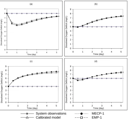
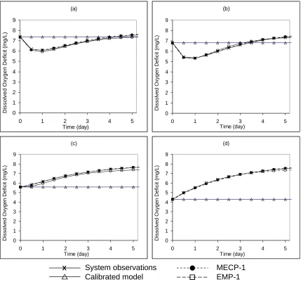
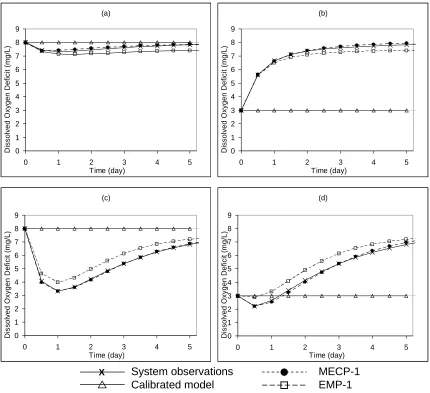
The DO deficit prediction performance of the three models in Table 2.3 for a portion of the training data, interpolation data, and validation data, are shown in Figs. 2.9, 2.10, and 2.11, respectively. The three figures reveal that calibration of the misspecified model does not simulate or predict the system observations well. For the training and interpolation data, MECP-1 and EMP-1 are both able to closely match the system

observations. Fig. 2.11 shows that outside of the training data, however, MECP-1 is able to predict the system response more closely than EMP-1.

Figure 2.8 Validation error for 30 random trials of MECP and GP-based search for

empirical model.

(31)

Table 2.3 Model details identified by three procedures. EMP-1 is best of thirty trials of GP-based search for empirical model.

MECP-1 is best of thirty trials of MECP.

Procedure Function

Predicted value for kd

(day-1)*

Training Error (mg/L) Validation Error (mg/L) Calibrated

Model - 0.00 3.66 5.83

EMP-1 - 0.31 0.73

MECP-1 0.47 0.11 0.28

(

0.75

)

75 . 0 0 88 . 0 45 . 0 0 75 . 1 80 . 0 exp 02 . 0 75 . 0 04 . 0 ' t t D D t D t

t ⎟⎟_⎠

⎞ ⎜ ⎜ ⎝ ⎛ − − + − +

(

)

(

)

(

t

)

_t t

tL

t D

t t

D 0.74

0

0 ₀_.₃₀

88 . 2 74 . 0 ln 30 . 0 60 . 0 60 . 0 ln 60 . 0 0 − − + + −

(32)

System observations Calibrated model output MECP-1 output

Empirical model output X (a) 0 1 2 3 4 5 6 7 8 9

0 1 2 3 4 5 Time (day) D is s o lv ed O x y gen D e fi c it ( m g /L) (b) 0 1 2 3 4 5 6 7 8 9

0 1 2 3 4 5

Time (day) Di ss ol v ed O x y g e n Def ic it ( m g/ L) (c) 0 1 2 3 4 5 6 7 8 9

0 1 2 3 4 5

Time (day) Di ss ol v ed O x y g e n Def ic it ( m g/ L) (d) 0 1 2 3 4 5 6 7 8 9

0 1 2 3 4 5

Time (day) Di ss ol v ed O x y g e n Def ic it ( m g/ L) System observations Calibrated model X MECP-1 EMP-1

Figure 2.9 Simulation capabilities of MECP-1, empirical model EMP-1, and calibrated

model for a portion of the training data (a) L = 20 mg/L, D = 0 mg/L, (b) L = 17.5 mg/L, D = 3 mg/L, (c) L = 10 mg/L, D = 4 mg/L, (d) L = 15 mg/L, D = 2 mg/L.

0 0 0

(33)

(a) 1 2 3 4 5 6 7 8 9 D issol ved O x yge n D e fi ci t ( m g/ L ) 0

0 1 2 3 4 5

Time (day) (b) 1 2 3 4 5 6 7 8 9 D iss o lve d O x y g en De fi c it (m g/ L ) 0

0 1 2 3 4 5

Time (day) (c) 0 1 2 3 4 5 6 7 8 9

0 1 2 3 4 5

Time (day) D iss olv ed Ox yge n D e fic it ( m g /L) (d) 0 1 2 3 4 5 6 7 8 9

0 1 2 3 4 5

Time (day) D iss olv ed Ox yge n D e fic it ( m g /L) System observations Calibrated model X MECP-1 EMP-1

Figure 2.10 Predictive capabilities of MECP-1, empirical model EMP-1, and calibrated

(34)

(a) 0 1 2 3 4 5 6 7 8 9 D is s ol ved Oxyg en D e fi ci t ( m g/ L )

0 1 2 3 4 5

Time (day) (b) 0 1 2 3 4 5 6 7 8 9 D is s ol ved Oxyg en D e fi ci t ( m g/ L )

0 1 2 3 4 5

Time (day) (c) 0 1 2 3 4 5 6 7 8 9

0 1 2 3 4 5

Time (day) Di ss ol v ed O x y g e n Def ic it ( m g /L) (d) 0 1 2 3 4 5 6 7 8 9

0 1 2 3 4 5

Time (day) Di ss ol v ed O x y g e n Def ic it ( m g /L) System observations Calibrated model X MECP-1 EMP-1

Figure 2.11 Predictive capabilities of MECP-1, empirical model EMP-1, and calibrated

model for extrapolated conditions (a) L0 = 5 mg/L, D0 = 0 mg/L, (b) L0 = 5 mg/L, D0 = 5

mg/L, (c) L0 = 35 mg/L, D0 = 0 mg/L, (d) L0 = 35 mg/L, D0 = 5 mg/L.

2.6 Final Remarks

The model error correction procedure is designed to search for parameter values and an error correction component to correct the output of a mechanistic model. Using a

(35)

and the structure of the empirical model mimics the true Streeter-Phelps model used to generate the training data. The empirical model does not, however, predict the validation data as well as MECP. Typically, empirical models do not predict well outside of

(36)

CHAPTER 3: An Evolutionary Algorithm to Generate Alternatives

(EAGA) for Engineering Optimization Problems

Abstract. Typically for a real optimization problem, the optimal solution to a

mathematical model of that real problem may not always be the “best” solution when considering unmodeled or unquantified objectives during decision-making. Formal approaches to explore efficiently for good but maximally different alternative solutions have been established in the operations research literature, and have been shown to be valuable in identifying solutions that perform expectedly well with respect to modeled and unmodeled objectives. While the use of evolutionary algorithms (EAs) to solve real engineering optimization problems is becoming increasingly common, systematic

alternatives generation capabilities are not fully extended for EAs. This paper presents a new EA-based approach to generate alternatives (EAGA), and illustrates its applicability via two test problems. A realistic airline route network design problem was also solved and analyzed successfully using EAGA. EAGA promises to be a flexible procedure for exploring alternative solutions that could assist when making decisions for real

engineering optimization problems riddled with unmodeled or unquantified issues.

3.1 Introduction

(37)

for making decisions about a solution to a real problem is questionable. In decision-making problems that are ill posed, all objectives may not be defined clearly (Liebman, 1976). This is a common issue in most public sector problems where the final decisions are shaped not just by the quantified objectives, but also by stakeholder preferences and social/political objectives that are subjective in nature. Such subjective considerations may not be expressed clearly, and therefore not quantitatively captured in the

optimization model.

A few algorithms have been designed to include subjective preferences in optimization through human interaction (e.g., Babbar et al., 2004; Bogardi and

Duckstein, 1992; Parmee and Bonham, 1999) to assist in steering the search. During the iterations of the algorithm, users view the solutions as they are generated and,

considering quantified and unquantified criteria, guide the search towards promising solutions. The application of such an interactive search approach to public sector problems is faced with many challenges. For example, the interactive approach works well when the turn-around time, i.e., time to generate a new solution, is sufficiently short such that the thought-process of the human is uninterrupted. In complex problems, typical of many engineering applications, long simulation model run times can render the solution turn-around time and interactive steering period excessive. In addition, as the size of the decision vector is characteristically large in most realistic engineering problems, the time a human evaluator takes to view and interpret a solution can

(38)

reshaped by the sequence of solutions that a human examines. Since the solution sequence is highly dependent upon initial conditions of the search algorithm, interactive steering will represent mostly local preference information.

When unmodeled objectives exist and cannot be incorporated through human interaction, different approaches are needed not only to search the decision space for the noninferior set of solutions to the optimization model being solved, but also to explore the decision space for alternative solutions. The following interesting and powerful observation was reported in (Brill, 1979) about the implications of unmodeled objectives on the decision space. Let the “optimal” solution to an SO model (with a quantified single-objective function Z1 that is being maximized) be X*corresponding to the optimal

objective function value Z1* (Fig. 3.1). Suppose Z2 (that is also being maximized) is an

unmodeled objective, such as social and political acceptability, that is not explicitly included in this SO model. If both Z1 and Z2 objectives were considered simultaneously

by the decision-maker when selecting the final solution, then, for example, the solution

XC, belonging to the 2-objective noninferior set, would represent a potential best

compromise solution. Although XC may be considered by the decision maker as the best

compromise solution to the real problem, in Z1 objective space it clearly appears inferior

to X* (since Z1C < Z1*). This argument can be extended similarly for an MOP model with

(39)

Z₁ Z₂

Z₁*

XC

Z₁C

X* Two-objective noninferior set

Figure 3.1 Illustration of a two-objective space.

Given these observations, the search for “good” solutions to a real optimization problem with unmodeled objectives should not be focused only on the noninferior set (or the optimal solution), but should also explore the inferior region to identify good

solutions. As described in (Brill, 1979), the Modeling to Generate Alternatives (MGA) approach implements a systematic exploration to generate a small number of alternative solutions that are good within the modeled objective space while being maximally different in the decision space. Resulting alternative solutions are likely to provide truly different choices, all performing similarly with respect to the modeled objectives but differently with respect to unmodeled objectives, enabling exploration of the decision space for good solutions while considering unmodeled objectives when making

(40)

The existing MGA approaches and applications are primarily based on mathematical programming-based search procedures. Research on EA-based MGA procedures is limited. As EAs are becoming a common solution approach to real problems, which typically consist of unmodeled objectives, more methodological development and application and testing of EA-based MGA procedures are needed.

The focus of this paper is to present a new EA-based approach for generating good alternative solutions. After describing the new algorithm, results are presented for two test problems. The new algorithm is then applied to a realistic airline routing

optimization problem that has several unmodeled decision criteria. Alternative solutions are compared and discussed in the context of selected unmodeled objectives.

3.2 Methodologies for Generating Alternatives

3.2.1 Foundation for Modeling to Generate Alternatives

The following is a formal definition of modeling to generate alternatives as provided in (Brill, 1979). Let the modeled optimization problem be represented as:

Minimize Z = f(X) (3.1)

Subject to gi(X) < bi ∀ i = 1, …, M (3.2)

where f(X) is the modeled objective function, Eqn. 3.2 represents the constraints, X (={xj,

j=1, …,N}) is the decision vector, N is the number of decision variables, and M is the

number of constraints. Suppose that the optimal solution to the above model is X*_with

an objective function value of Z*. To generate an alternative solution that is maximally different from X*, the following model is solved:

Maximize D = Σj | xj – xj* | (3.3)

(41)

f(X) < T(Z*) (3.5)

where D is a difference function, and T is a target that is specified in relation to the optimal function value Z*. T represents how much of the inferior region is to be explored for alternative solutions. For example, if the original objective is to minimize cost and the least cost is $1 M, then the target could be set at $1.1 M, allowing for solutions that are no more than 10% over the optimal solution. To generate additional alternatives, the difference function D is modified such that the new solution being sought is maximally different from all previous solutions, while Eqns. 3.4 and 3.5 remain unchanged. The search for alternatives stops when either no new alternative solution is found or a sufficient number of alternatives are generated.

A number of different approaches, all based on mathematical programming-based search methods (including linear programming, nonlinear programming, integer/binary programming, and dynamic programming), for generating a sequence of alternative solutions is described in (Chang et al., 1982), (Nakamura and Brill, 1977), and (Brill et al., 1982).

3.2.2 EA-based Search Approaches for Alternatives Generation

(42)

More elegant procedures that exploit the EA’s ability to represent multiple different solutions simultaneously will likely be more efficient. One potential approach utilizes the niching operator (Mahfoud, 1995) through fitness sharing in decision space to generate a number of alternatives (Loughlin et al., 2001). By adjusting the sharing distance parameter or the niche count, the niche size and therefore the number of niches (or alternative solutions) can be changed. Although this requires setting of additional parameter values, multiple solutions can be represented in the population and a set of good solutions can be identified simultaneously. The drawback, however, is that during the search the alternative solutions are not ensured to be as far apart from each other as possible in the decision space, a primary goal of generating a small set of relatively good but maximally different solutions. To overcome this shortcoming, (Loughlin et al., 2001) suggests a post-screening step to select from among the different niches a few

alternatives that are maximally different with respect to some difference measure. A GA-based procedure (GAMGA – Genetic Algorithms for Modeling to Generate Alternatives) presented in (Loughlin et al., 2001) sorts the population after each

(43)

A new EA-based approach for generating alternatives, as described below, attempts to overcome the existing shortcomings and provide a generic and flexible procedure with several added advantages.

3.3 An Evolutionary Algorithm to Generate Alternatives (EAGA)

EAGA, which is designed to generate a small number of good but maximally different alternatives, is built upon the basic concepts of co-evolution. In this new algorithm, subpopulations collectively search for different alternative solutions. Each solution is represented by one subpopulation that undergoes an evolutionary search procedure. This search can be structured based on any standard evolutionary search procedure with the appropriate encoding and operators that best suit the problem being solved. The survival of solutions in each subpopulation depends upon how well the solutions perform with respect to the modeled objective(s) as well as upon how far they are from the other solutions in decision space. Thus, the evolution of solutions in a subpopulation is influenced by those in the other subpopulations, forcing migration of each subpopulation towards good but distant regions of the decision space. This enables the design of an explicit algorithm to search for a set of good solutions that are maximally different from each other.

While EAGA is applicable to higher dimensional (multiobjective) optimization problems, this algorithm is described here for generating maximally different alternative solutions specifically to single-objective optimization problems. The man steps of the algorithm are described below.

Step 1. Initialization – create an initial population with P subpopulations (each with a

(44)

value for P is typically assigned by the user or the decision-maker. Let SPp (p=1, …,P)

represent the index for subpopulation p. The first subpopulation (SP1) is dedicated to the

search for the optimal solution to the modeled problem, and this solution will serve as the benchmark for setting the relaxation constraint Eqn. 3.5, which is also specified by the user.

Step 2. In SP1, evaluate and identify the best solution with respect to the modeled

objective.

Step 3. In SPp, p=2, …, P, evaluate all solutions with respect to the modeled objective.

Solutions that meet the target constraint Eqn. 3.5 are assigned a “feasible” flag, and the others an “infeasible” flag.

Step 4. Apply an elitism operator to all subpopulations SPp to preserve the best

individual in each subpopulation. In SP1, the best individual is defined as the solution

that performs best with respect to the modeled objective. In SPp, p=2, …, P, the best

individual will be a feasible solution that is located most distantly in decision space from the other subpopulations. The distance measure that is used to identify the most distant individual in a subpopulation is defined in Step 7. If all solutions in a subpopulation are infeasible, then the best individual is the solution that performs best with respect to the modeled objective.

Step 5. Check for termination criteria. Stop the algorithm if termination criteria (e.g., a

maximum number of iterations) are met. Otherwise, go to Step 6.

Step 6. For each SPp, identify the centroid in decision space. The centroid may be

defined as the simple average, { cip = (1/K) Σk xik,p ; i=1, …,N }, where cip is the centroid

(45)

solution k in subpopulation p, and N is the number of decision variables. Alternatively, the centroid may be defined as a fitness-weighted average { cip = (1/K) Σk Fk,pxik,p ; i=1, …,N }, where Fk,p is the fitness of solution k in subpopulation p.

Step 7. For each solution k in subpopulation SPq(q≠1), calculate a distance measure Dk,q

in the decision space between that solution and other subpopulations. A simple distance measure is Dk,q = Min { Σi |xik,q – cip| ; p=1,...,P, p≠q}. This distance represents the

minimum distance between solution k in subpopulation q and the centroids of all other subpopulations.

Step 8. In each subpopulation SPp, apply binary tournament selection. In SP1, the

selection is based on how good the solution is with respect to the modeled objective(s). In SPp, p≠1, the selection is based on the fitness of the solution with respect to the

modeled objective(s) (i.e., meeting constraint Eqn. 3.5) as well as its distance from other subpopulations (Dk,p). In the binary tournament, when both solutions are feasible with respect to the relaxation target constraint Eqn. 3.5, the one with the better objective function value is selected. In all other cases, the selection criterion is applied adaptively depending on feasibility characteristics of each subpopulation. If the majority of the solutions in that subpopulation are infeasible with respect to the relaxation target, then the selection is based on the objective function value. Otherwise, the selection is based on the distance measure Dk,p.

Step 9. In each subpopulation, apply recombination operators to the solutions selected in

(46)

3.4 One-Dimensional Test Problem

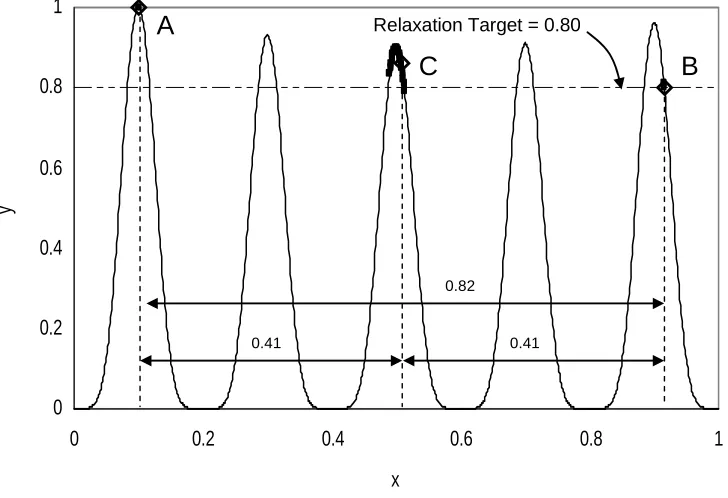
The first test problem maximizes a one-dimensional, sinusoidal function with five peaks (Eqn. 3.6, Fig 3.2). This function was adapted from a function that has been acknowledged as a preliminary benchmark for niching GA’s (Mahfoud, 1995).

y(x) = (0.5(x – 0.55)2 + 0.9)sin6(5πx) (3.6)

The optimal solution to this simple problem is A (at x=0.1) with a function value of 1. The maximally different (i.e., farthest in decision space) alternative solution that is within a 20% relaxation target (i.e., y(x) > 0.8 is point B (Fig 3.2)). B and C (at x=0.51)

collectively represent the most different set of two alternatives.

0 0.2 0.4 0.6 0.8 1

0 0.2 0.4 0.6 0.8

x

y

0.82

0.41 0.41

Relaxation Target = 0.80

A

C

B

1

Figure 3.2 Objective and decision space for the one-dimensional test problem. A, B, and

C represent the set of three maximally different alternative solutions for a 20% relaxation target. Points represent solutions obtained using EAGA for thirty random trials.

(47)

successfully to the best set of alternatives, A, B, and C. The parameter settings for EAGA are listed in Table 3.1. To examine the sensitivity of the convergence of the algorithm, thirty random trials of the three-subpopulation case were conducted. All solutions are plotted in Fig. 3.2. While convergence to A and C is consistent, a slight variation in convergence to B is observed.

Table 3.1 EAGA parameter settings for the test problems and the airline problem.

Parameter Test Problems Airline Problem

Population Size 100 100

Number of Generations 100 100

Crossover 60% 40%

Mutation 5% 5%

Decision Variable Representation Real Integer

3.5 Two-Dimensional Test Problem

A two-dimensional multi-modal test problem (Loughlin et al., 2001) maximizes the following function:

F(x,y) = sin(19πx) + x/1.7 + sin(19πy) + y/1.7 +2 (3.7)

The objective and decision spaces are shown in Fig. 3.3. The objective landscape has 100 peaks, increasing in height from one corner (0,0) to the opposite corner (1,1). The

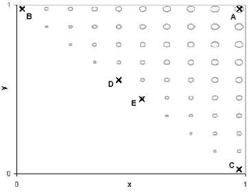
highest peak is indicated by A (f(x,y) = 5.146. x = 0.974, y = 0.974). Considering a relaxation of 12%, the target relaxation constraint Eqn. 3.5 is F(x,y) > 4.528 (i.e., 12% less than the optimal value 5.146). Fig 3.3 also shows projections (on the x-y plane) of the feasible search space meeting this relaxation constraint. Fig 3.4 shows the decision space and the best set of four alternative solutions. A (0.974, 0.974) is the global

(48)

difference for a set of four solutions has been defined as the average distance between each pair of solutions in the set based on the Euclidean distance in decision space. EAGA was set up with four subpopulations (with parameter settings as shown in Table 3.1). The best solution from each subpopulation produced the set of points A, B, C, and D, the best set of four solutions to this problem. The progression of the subpopulations in the decision space is plotted in Fig. 3.5. The first subpopulation converges fairly early to the highest peak, A. As this subpopulation finds its place in the decision space, the others move away from it as well as away from each other. While the third and the fourth subpopulations migrate towards B and C, the second subpopulation converges slowly, and relatively weakly, which may be due to the presence of two equally good and different solutions (D and E).

(49)

A

f(x,y)

Figure 3.3 Objective landscape of the two-dimensional test function, with feasible

(50)

Figure 3.4 Decision space at 12% relaxation for the two-dimensional test problem. The

(51)

0 1

0 _x 1

y 0 1 0 1 x y 0 1

0 _x 1

y 0 1 0 1 x y 0 1

0 _x 1

y 0 1 0 1 x y 0 1

0 _x 1

y 0 1 0 1 x y 0 1

0 _x 1

y

0 1

0 _x 1

y

0 1

0 _x 1

y 0 1 0 1 x y 0 1

0 _x 1

y

0 1

0 _x 1

y

0 1

0 _x 1

y 0 1 0 1 x y 0 1

0 _x 1

y

0 1

0 _x 1

y 0 1 0 1 x y 0 1

0 _x 1

y 0 1 0 1 x y 0 1 0 1 x y 0 1 0 1 x y 0 1 0 1 x y

Subpopulation 1 Subpopulation 2 Subpopulation 3 Subpopulation 4

1 10 25 50 100 5 Generation Number

Figure 3.5 Distribution of the solutions in each subpopulation at the end of generations 1,

(52)

0 0.1 0.2 0.3 0.4 0.5 0.6 0.7 0.8 0.9 1

0.065 0.13 0.26 0.52 0.65

M

e

a

n

D

iff

er

en

ce

sigma share

Niching GA with post screening* GAMGA* EAGA

Figure 3.6 Comparison of performance of alternative solutions obtained using GAMGA, a niching with post screening procedure, and EAGA for the two-dimensional test

problem. The error bars represent the difference range based on 100 random trials.

Note: * - data source (Loughlin et al., 2001)

3.6 Application to an Airline Route Network Design Problem

A realistic airline route network design problem, which was reported in (Brill et

al., 1990), is used to test and demonstrate the application of EAGA. The design goal is to

find a cost-effective set of airline routes connecting eight cities as shown in Fig. 3.6:

Atlanta (ATL), Baltimore (BAL), Boston (BOS), Chicago (CHI), Cincinnati (CIN),

Cleveland (CLE), Dallas Fort Worth (DFW), and Houston (HOU). The demands for

travel between pairs of cities are shown in Table 3.2. The cost of a link, or a flight path,

between two cities includes an initial cost of set up ($6M per link) and a unit cost per

passenger trip as shown in Table 3.3. The solution space represents combinations of

(53)

connecting every pair of cities. Some pairs of cities may be connected directly, while some others may be connected with multiple legs via other cities.

Figure 3.7 Airline network of eight cities.

This combinatorial search problem was modeled as a binary linear programming (BLP) model, as shown below, and solved using a branch-and-bound algorithm (Brill et al., 1990).

Minimize ΣiΣj>i [ cij(Σk≠jXijk + Σk≠ iXjik ) + fijdij] (3.8)

Subject to Σj ≠iXjik−Σj ≠i,kXijk= Dij ∀i, k≠i (3.9)

Xijk≥ 0 ∀ i, j ≠i, k≠i (3.10)

dij∈{ 0,1 } ∀ i, j ≠i, k≠i (3.11)

where

Xijk= the number of passenger trips in the link connecting cities i and j which originated

(54)

dij = a Boolean variable, equals 1 if the link connecting cities i and j is open and 0

otherwise

cij= incremental cost per single passenger between cities i and j fij= fixed cost of opening the link between cities i and j

Dij= estimated passenger-trips per year between cities i and j

The objective function (Eqn. 3.8) represents the total cost of the network and the constraint set in Eqn. 3.9 represents the flow balance in the network.

Table 3.2 Demand in passenger-trips per year

ATL BAL BOS CHI CIN CLE DFW HOU

ATL - 6480 7640 20060 4690 6200 11700 7260

BAL 6480 - 13010 13710 3330 5580 3880 4200

BOS 7640 13010 - 35170 5960 14130 5960 4250

CHI 20060 13710 35170 - 19110 35150 21440 15840

CIN 4690 3330 5960 19110 - 7290 3110 1920

CLE 6200 5580 14130 35150 7290 - 5030 3550

DFW 11700 3880 5960 21440 3110 5030 - 34290

HOU 7260 4200 4250 15840 1920 3550 34290 -

Table 3.3 Incremental cost in $/passenger-trip per year

ATL BAL BOS CHI CIN CLE DFW HOU

ATL - 57.7 94.65 59.76 37.38 55.98 70.9 69.52

BAL 57.7 - 36.95 61.3 42.91 31.29 119.65 124.2

BOS 94.65 36.95 - 85.83 74.96 55.61 154.13 160.32

CHI 59.76 61.3 85.83 - 25.5 31.13 79.01 93.22

CIN 37.38 42.91 74.96 25.5 - 22.59 79.42 87.96

CLE 55.98 31.29 55.61 31.13 22.59 - 100.97 110.46

DFW 70.9 119.65 154.13 79.01 79.42 100.97 - 22.14

HOU 69.52 124.2 160.32 93.22 87.96 110.46 22.14 -

(55)

different alternative solutions can be found in a slightly inferior region if the airline were to spend a small percentage (10%) over the least cost, and how these different solutions perform with respect to the many unmodeled but important decision criteria.

This problem was solved using EAGA to identify the least-cost solution and a set of three alternatives that are maximally different from the least-cost and each other. These solutions are then compared with respect to the following unmodeled objectives: convenience related to direct vs. multi-leg flights, and potential for delays.

3.6.1 Surrogates for Unmodeled Objectives

To enable a quantitative comparison of the alternative solutions with respect to these unmodeled objectives, the following surrogates, identified by (Brill et al., 1990), are used in this study. The total number of stop-overs is used to represent the level of inconvenience caused by flights that are not direct. The total number of passenger-trips handled at each city is used to denote the level of congestion and therefore potential delays that may arise due to unexpected airport closures. While these quantitative surrogates could have been modeled explicitly within the optimization model as a multiobjective problem, they are considered here as unmodeled issues for illustrative purposes. As there exist several other truly unquantifiable design criteria, the general approach for examining alternative solutions in consideration of unmodeled objectives would follow the illustration presented here.

3.6.2 Results and Discussion

(56)

3.1. The resulting set of networks is given in Fig. 3.8, which also shows the cost and number of stop-overs for each alternative network. The thickness of the links in each network is drawn proportional to the total number of passenger trips in that link.

(57)

HOU DFW CHI CIN CLE BAL ATL BOS $90.9 Million HOU DFW CHI CIN CLE BAL ATL BOS $99.7 Million HOU DFW CHI CIN CLE BAL ATL BOS $99.6 Million HOU DFW CHI CIN CLE BAL ATL BOS $100.0 Million