| INVESTIGATION
Inference of Gene Flow in the Process of Speciation:
An Ef
fi
cient Maximum-Likelihood Method for the
Isolation-with-Initial-Migration Model
Rui J. Costa1and Hilde Wilkinson-Herbots Department of Statistical Science, University College London, WC1E 6BT, United Kingdom
ABSTRACT The isolation-with-migration (IM) model is commonly used to make inferences about geneflow during speciation, using polymorphism data. However, it has been reported that the parameter estimates obtained byfitting the IM model are very sensitive to the model’s assumptions—including the assumption of constant geneflow until the present. This article is concerned with the isolation-with-initial-migration (IIM) model, which drops precisely this assumption. In the IIM model, one ancestral population divides into two descendant subpopulations, between which there is an initial period of geneflow and a subsequent period of isolation. We derive a very fast method offitting an extended version of the IIM model, which also allows for asymmetric geneflow and unequal population sizes. This is a maximum-likelihood method, applicable to data on the number of segregating sites between pairs of DNA sequences from a large number of independent loci. In addition to obtaining parameter estimates, our method can also be used, by means of likelihood-ratio tests, to distinguish between alternative models representing the following divergence scenarios: (a) divergence with potentially asymmetric gene flow until the present, (b) divergence with potentially asymmetric gene flow until some point in the past and in isolation since then, and (c) divergence in complete isolation. We illustrate the procedure on pairs ofDrosophilasequences from30,000 loci. The computing time needed tofit the most complex version of the model to this data set is only a couple of minutes. The R code tofit the IIM model can be found in the supplementary
files of this article.
KEYWORDSspeciation; coalescent; maximum-likelihood; geneflow; isolation
T
HE two-deme, isolation-with-migration (IM) model is a population genetic model in which, at some point in the past, an ancestral population divided into two subpopulations. After the division, these subpopulations exchanged migrants at a constant rate until the present. The IM model has become one of the most popular probabilistic models in use to study genetic diversity under geneflow and population structure. Although applicable to populations within species, many researchers are using it to detect geneflow between divergingpopulations and to investigate the role of gene flow in the process of speciation. A meta-analysis of published research articles that used the IM model in the context of speciation can be found in Pinho and Hey (2010).
Several authors have developed computational methods to
fit IM models to real DNA data. Some of the most-used programs are aimed at data sets consisting of a large number of sequences from a small number of loci. This is the case of MDIV (Nielsen and Wakeley 2001), IM (Hey and Nielsen 2004; Hey 2005), IMa (Hey and Nielsen 2007), and IMa2
(Hey 2010), which rely on Bayesian Markov chain Monte Carlo (MCMC) methods to estimate the model parameters and are computationally very intensive.
In the past decade, the availability of large data sets spanning the entire genome has increased significantly. How-ever, the MCMC-based implementations of the IM model referred to above are computationally expensive even for small numbers of loci, and their running times increase linearly with the number of loci (Wang and Hey 2010). Copyright © 2017 Costa and Wilkinson-Herbots
doi:https://doi.org/10.1534/genetics.116.188060
Manuscript received May 11, 2016; accepted for publication January 25, 2017; published Early Online February 13, 2017.
Available freely online through the author-supported open access option.
This is an open-access article distributed under the terms of the Creative Commons Attribution 4.0 International License (http://creativecommons.org/licenses/by/4.0/), which permits unrestricted use, distribution, and reproduction in any medium, provided the original work is properly cited.
Supplemental material is available online atwww.genetics.org/lookup/suppl/doi:10. 1534/genetics.116.188060/-/DC1.
1Corresponding author: Department of Statistical Science, University College London,
Fitting an IM model also provides a rather simplified picture of the divergence process, which for some research purposes is clearly insufficient (for example, if one wishes to know whether a process of sympatric speciation has been com-pleted, or whether geneflow occurred due to secondary contact). In addition, Becquet and Przeworski (2009) and Strasburg and Rieseberg (2010) showed that inference based on the programsIMandIMacan become unreliable if any of the assumptions made about population struc-ture, recombination, or linkage is severely violated. For these reasons, there has been a significant increase in the demand for methods that not only scale well to genome-sized data, but are also able to estimate increasingly re-alistic models.
To improve efficiency and scalability, one possible strat-egy is to work with summary statistics rather than full data patterns. The MCMC-based program MIMAR of Becquet and Przeworski (2007, 2009) uses the four summary statistics studied by Wakeley and Hey (1997) tofit the IM model, and drops the assumption of no intralocus recombination. Gutenkunst et al. (2009) introduced a method based on the joint sample frequency spectrum (JSFS) that is able to
fit a range of demographic models incorporating multiple populations, periods of migration and admixture, splits and joins of populations, and changes in population sizes. Based on the same type of data, the more recent implementation of Kammet al.(2016) can already deal with a large number of individuals and populations, but does not yet include gene
flow.
Genome-scale data sets, even when stemming from just a few individuals, tend to be more informative than data sets consisting of many individuals but covering only a relatively short genomic region. In fact, as the sample size for a single locus increases, the probability that an extra sequence adds a deep (i.e., informative) branch to the coalescent tree quickly becomes negligible (see for example Heinet al.2005, pp. 28– 29). Data sets of a small number of individuals per locus are also more suitable for likelihood-based inference: if at each locus the observation consists only of a few sequences, the coalescent process of these sequences is relatively simple and can more easily be used to derive the likelihood for the locus concerned.
Among the methods designed for whole-genome se-quence data of only a few individuals are those of Mailund
et al.(2012), Schiffels and Durbin (2014), and Steinrücken
et al.(2015). The fact that they are designed for full poly-morphism data makes these methods computationally more expensive than JSFS-based methods. However, they rely on the coalescent with recombination modeled as a hidden Markov process,i.e., they are able to capture the linkage information present in the data. Presently, com-plex models of demographic history can already befitted using this approach (see, for example, Steinrückenet al.
2015).
Arguably the only implementations that can be considered
fastare those based onblockwise-likelihoodmethods. These
implementations are also aimed at a small number of sam-pled individuals, and use the information in each of a large number of relatively short and well separated loci: because recombination within loci is disregarded, it is considerably easier to derive explicitly the likelihood for each locus; and because linkage between loci is assumed to be negligible, the likelihood of a data set is just the product of the likelihoods for the individual loci.
Blockwise-likelihood methods for the standard two-deme IM model have been developed, for example, by Wilkinson-Herbots (2008) and Wang and Hey (2010), for pairs of DNA sequences at a large number of indepen-dent loci, and by Lohseet al.(2011) and Andersenet al.
(2014) for larger numbers of sequences at each locus. Lohseet al. (2011) also developed a more general Laplace-transform method to calculate blockwise likelihoods for a range of demographic scenarios, which was further ex-tended and efficiently automated in Lohse et al.(2016). Zhu and Yang (2012) developed an implementation, based on triplets of sequences, of an IM model with three species with known phylogeny and symmetric migration between two of them.
Some authors have focused on blockwise-likelihood meth-ods for models of divergence that drop the assumption of constant geneflow until the present, and which are therefore more realistic in the context of speciation. In particular, Innan and Watanabe (2006) considered a model in which the level of gene flow between two subpopulations gradually de-creases until they become completely isolated from each other. Their calculation of the likelihood of the number of nucleotide differences between pairs of sequences relies on the numerical computation of the coalescence time density at different points in time, which can be computationally expen-sive. IM models in which gene flow is allowed to cease at some point in the past—hereafter referred to as isolation-with-initial-migration (IIM) models—have also been consid-ered by, for example, Teshima and Tajima (2002), Becquet and Przeworski (2009), Mailund et al. (2012), Wilkinson-Herbots (2012), and Lohseet al.(2015).
In the present article, we apply matrix eigen-decomposition techniques to expand on the work of Wilkinson-Herbots (2012) on the IIM model, who derived explicit formulas for the dis-tribution of the coalescence time of a pair of sequences, and the distribution of the number of nucleotide differences be-tween them. These analytic results enable a very fast compu-tation of the likelihood under an IIM model, given a data set consisting of observations on pairs of sequences at a large number of independent loci (Lohse et al.2015; Wilkinson-Herbots 2015; Jankoet al.2016). However, for mathematical reasons, this work adopted two biologically unrealistic as-sumptions which may affect the reliability of estimates: sym-metric migration and equal subpopulation sizes during the migration period.
well as during the isolation stage. Both this model and other simpler models studied in this article assume haploid DNA sequences, which accumulate mutations according to the infinite-sites assumption (Watterson 1975). An extension to the Jukes–Cantor model of mutation is feasible but beyond the scope of this article.
We first describe an efficient method to compute the likelihood of a set of observations on the number of nucle-otide differences between pairs of sequences, where each pair comes from a different locus and where we assume free recombination between loci and no recombination within loci. As our method uses an explicit expression for the likeli-hood, it is very fast, and efficient enough to easily deal with asymmetric bidirectional gene flow, unequal population sizes, mutation rate heterogeneity, and large numbers of mutations. Second, we illustrate how to use this method tofit the IIM model to real data. The data set ofDrosophila
sequences from Wang and Hey (2010), containing over 30,000 observations (i.e., loci), is used for this purpose. Finally we demonstrate, using this data set, how different models representing different evolutionary scenarios can be compared using likelihood-ratio tests. More specifically, we compare three main scenarios: (a) divergence without gene
flow; (b) divergence with potentially asymmetric geneflow until the present; and (c) divergence with potentially asym-metric geneflow until some time in the past, and in isolation since then.
Methods
For the purposes of the present article, and from a forward-in-time perspective, the IM model makes the following assump-tions: (a) until time t0 ago ðt0.0Þ; a population of DNA sequences from a single locus followed a Wright–Fisher hap-loid model (Fisher 1930; Wright 1931); and (b) at timet0 ago, this ancestral population split into two Wright–Fisher subpopulations with constant gene flow between them. If we take an IM model and add the assumption that, at time
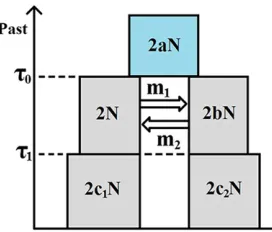
t1agoð0,t1,t0Þ;geneflow ceased, we get an IIM model. Figure 1 illustrates the fullest IIM model dealt with in this article.
In the IIM model of Figure 1, the population sizes are given inside the boxes, in units of DNA sequences. All population sizes are assumed constant and strictly positive. The param-etersa,b,c1;andc2 indicate the relative size of each popu-lation with respect to subpopupopu-lation 1 during the migration stage. For example, if 2Nancis the number of sequences in the ancestral population, thena¼2Nanc=2N:Between timest0 andt1ago (two time parameters in units of 2Ngenerations), there is geneflow between the subpopulations: in each gen-eration, a fractionmiof subpopulationiare immigrants from subpopulationjði;j2 f1;2gwithi6¼jÞ;i.e.,miis the migra-tion rate per generamigra-tion from subpopulamigra-tionito subpopula-tion j backward in time. Within each subpopulation, reproduction follows the neutral Wright–Fisher model and, in each generation, restores the subpopulations to their
orig-inal sizes,i.e., reproduction undoes any decrease or increase in size caused by geneflow.
Under the IIM model, the genealogy of a sample of two DNA sequences from the present subpopulations can be described by successive Markov chains, working backward in time. We will define these in the simplest possible way, using the small-est state space necessary for the derivation of the coalescence time distribution. Hence, during the isolation stage (until time
t1into the past) and the migration stage (betweent1andt0Þ; the process can only be in state 1—both lineages in subpop-ulation 1, state 2—both lineages in subpopulation 2, state 3—one lineage in each subpopulation, or state 4—in which lineages have coalesced. After t0; the lineages have either coalesced already—state 4, or have not—state 0. Only states 1, 2, and 3 can be initial states, according to whether we sample two sequences from subpopulation 1, two sequences from subpopulation 2, or one sequence from each subpopu-lation. When the genealogical process starts in state i ðwithi2 f1;2;3gÞ;the time until the most recent common ancestor of the two sampled sequences is denoted TðiÞ; whereas SðiÞ denotes the number of nucleotide differences between them.
If time is measured in units of 2N generations andNis large, the genealogical process is well approximated by a succession of three continuous-time Markov chains; one for each stage of the IIM model (Kingman 1982a,b; Notohara 1990). We refer to this stochastic process in continuous time as thecoalescentunder the IIM model. During the isolation stage, the approximation is by a Markov chain defined by the generator matrix
(1)
withi2 f1;2gbeing the initial state (Kingman 1982a,b). If 3 is the initial state, the lineages cannot coalesce beforet1: During the ancestral stage, the genealogical process is ap-proximated by a Markov chain with generator matrix
(2)
(Kingman 1982a,b). In between, during the migration stage, the approximation is by a Markov chain with generator matrix
(3)
(Notohara 1990). In this matrix,Mi=2¼2Nmi represents the rate of migration (in continuous time) of a single sequence when in subpopulationi. The rates of coalescence for two lineages in subpopulation 1 or 2 are 1 and 1=b;respectively. Note that state 3 corresponds to the second row and column, and state 2 to the third row and column. This swap was dictated by mathematical convenience: the matrixQmigshould be as symmetric as possible
because this facilitates a proof in the next section. Distribution of the time until coalescence under bidirectional geneflow (M1>0, M2>0)
TofindfTðiÞ;the density of the coalescence timeTðiÞof two
line-ages under the IIM model, given that the process starts in statei
and there is geneflow in both directions, we consider separately the three Markov chains mentioned above. We let TisoðiÞ
ði2 f1;2gÞ;TmigðiÞ ði2 f1;2;3gÞ;andT ð0Þ
ancdenote the times until absorption of the time-homogeneous Markov chains defined by the generator matricesQðisoiÞ;Qmig;andQanc;respectively.
Fur-thermore, we let the corresponding probability density functions (PDFs) [or cumulative distribution functions (CDFs)] be denoted byfisoðiÞ;fmigðiÞ;andfancð0Þ (orFð
iÞ iso;F
ðiÞ
mig;andF
ð0Þ
ancÞ:Then,fð
iÞ
T can be
expressed in terms of the distribution functions just mentioned:
fTðiÞðtÞ ¼
fisoðiÞðtÞ for 0#t#t1;
h
12FisoðiÞðt1ÞifmigðiÞðt2t1Þ fort1,t#t0;
h
12FisoðiÞðt1Þih12FðiÞmigðt02t1Þifancð0Þðt2t0Þ fort0,t,N;
0 otherwise;
8 > > > > < > > > > : (4)
fori2 f1;2g:If 3 is the initial state,
fTð3ÞðtÞ ¼
8 > < > :
fmigð3Þðt2t1Þ fort1,t#t0; h
12Fðmig3Þðt02t1Þ i
fancð0Þðt2t0Þ fort0,t,N;
0 otherwise:
(5)
The important conclusion to draw from these considerations is that tofind the distribution of the coalescence time under the IIM model, we only need to find the distributions of the absorption times under the simpler processes just defined.
A Markov process defined by the matrixQanc;and starting in
state 0, is simply Kingman’s coalescent (Kingman 1982a,b). For such a process, the distribution of the coalescence time is exponen-tial, with rate equal to the inverse of the relative population size:
fancð0ÞðtÞ ¼ 1
ae
2ð1=aÞt; 0#t,N: (6)
A Markov process defined byQðisoiÞ;i2 f1;2g;is again King-man’s coalescent, so
fisoðiÞðtÞ ¼1 ci
e2ð1=ciÞt; 0#t,N: (7)
Finally, with respect to the “structured”coalescent process defined by the matrixQmig; we prove in Appendix A that,
fori2 f1;2;3g;
fmigðiÞðtÞ ¼ 2X
3
j¼1
Vij21Vj4lje2ljt; (8)
whereVijis theði;jÞentry of the (nonsingular) matrixV;whose rows are the left eigenvectors of Qmig:Theði;jÞ entry of the
matrix V21 is denoted byV21
ij :Thelj ðj2 f1;2;3gÞare the
absolute values of those eigenvalues ofQmig which are strictly
negative (the remaining one is zero). Since theljare real and
strictly positive, the density function ofTmigðiÞ is a linear combi-nation of exponential densities.
Substituting the PDFs from Equations 6, 7, and 8 into the Equations 4 and 5, and denoting by A the three-by-three matrix with entriesAij¼ 2V21
ij Vj4;we obtain
fTðiÞðtÞ ¼
1
cie 21
cit for 0#t#t1;
e2ci1t1P3
j¼1
Aijlje2ljðt2t1Þ fort1,t#t0;
e2ci1t1P3
j¼1
Aije2ljðt02t1Þ 1
ae
21
aðt2t0Þ fort0,t,N;
0 otherwise;
8 > > > > > > > > > > > > < > > > > > > > > > > > > : (9) fori2 f1;2g;and
fTð3ÞðtÞ ¼
P3
j¼1
A3jlje2ljðt2t1Þ fort1,t#t0;
P3
j¼1
A3je2ljðt02t1Þ 1
ae
21
aðt2t0Þ fort0,t,N;
0 otherwise:
8 > > > > > > > < > > > > > > > : (10)
results 9 and 10 above simplify to the corresponding results in Wilkinson-Herbots (2012)—in this case, the coefficientAi3 in the linear combination is zero fori2 f1;2;3g:
Distribution of the time until coalescence under
unidirectional geneflow, and in the absence of geneflow
If eitherM1orM2is equal to zero, or if both are equal to zero, the above derivation offmigðiÞ is no longer applicable,
as the similarity transformation in Part (ii) of the proof (Appendix A) is no longer defined (see the denominators in some entries of the matrixD). In this section, we derive
fmigðiÞ;the density of the absorption time of the Markov chain defined by the matrixQmig given in Equation 3, starting
from state i, when one or both the migration rates are zero. Again, this is all we need tofill in Equations 4 and 5 and obtain the distribution of the coalescence time of a pair of DNA sequences under the IIM model. Having geneflow in just one direction considerably simplifies the coalescent. For this reason, we resort to moment-generating functions (MGFs), instead of eigen-decomposition, and derive fully explicit PDFs.
Let TmigðiÞ again be defined as the absorption time of the Markov chain generated by Qmig; now with M1¼0 and
M2.0;given that the initial state isi2 f1;2;3g:We condi-tion on the state of the coalescent after thefirst transition to obtain the following system of equations for the MGF ofTmigðiÞ; wheresdenotes a dummy variable:
E n
exp h
2sTðmig1Þ
io
¼ 1
1þs
!
Enexph2sTðmig2Þio¼ M2
1=bþM2þs !
Enexph2sTðmig3Þio
þ 1=b
1=bþM2þs !
E n
exp h
2sTðmig3Þ
io
¼ M2
M2þ2s !
E n
exp h
2sTmigð1Þ
io
(see also more general equations in Wilkinson-Herbots 1998 and Lohseet al.2011). Solving this system of equa-tions and applying a partial fraction decomposition (anal-ogous to the work done in Griffiths 1981 and Nath and Griffiths 1993, for the case of symmetric migration and equal population sizes), the distributions of Tmigð1Þ; T
ð2Þ mig; andTmigð3Þ can be expressed as linear combinations of expo-nential distributions:
Thus we obtain the following PDFs:
fmigð1ÞðtÞ ¼e2t
fmigð2ÞðtÞ ¼
"
bM22
ðM222Þð12bþbM2Þ #
e2t
þ
"
4bM2
ð22M2Þð2þbM2Þ #
M2 2 e
2M2
2t
þ
" 1 1þbM2
þ b2M22
ð2þbM2Þð12bþbM2Þð1=bþM2Þ #
3 1
bþM2
!
e2ð1=bþM2Þt
fmigð3ÞðtÞ ¼ M2 M222
!
e2tþ 2
22M2 !
M2 2 e
2M2 2t
fort.0:
The PDF of the coalescence time of a pair of DNA sequences under an IIM model withM1¼0 andM2.0 can now be easily derived by comparing the above expressions with Equation 8:
fTðiÞðtÞis given by Equations 9 and 10 above, but now with
l¼
" 1 M2
2 1
bþM2
#
;
and
In the opposite case of unidirectional migrationðM1.0;M2¼0Þ; we obtained the distribution of the time until coalescence E
n exp
h 2sTmigð1Þ
io
¼ 1
1þs
!
E n
exp h
2sTmigð2Þ
io
¼ M2 1=bþM2þs
!
M2
M2þ2s !
1 1þs
!
þ 1=b
1=bþM2þs !
¼
"
bM22
ðM222Þð12bþbM2Þ #
1 1þs
!
þ
"
4bM2
ð22M2Þð2þbM2Þ #
M2
M2þ2s !
þ
" 1=b
1=bþM2þ
b2M22
ð2þbM2Þð12bþbM2Þð1=bþM2Þ #
1=bþM2 1=bþM2þs
!
E n
exp h
2sTmigð3Þ
io
¼ M2
M2þ2s !
1 1þs
!
¼ M2
M222 !
1 1þs
!
þ 2
22M2 !
M2
M2þ2s !
using essentially the same procedure as described above. In addition, forM1¼M2¼0;the derivation is trivial. The results for these two cases can be found in Appendix B.
The distribution of the number S of segregating sites
LetSðiÞdenote the number of segregating sites in a random sample of two sequences from a given locus, when the ances-tral process of these sequences follows the coalescent under the IIM model and the initial state is state iði2 f1;2;3gÞ: Recall the infinite-sites assumption and assume that the dis-tribution of the number of mutations hitting one sequence in a single generation is Poisson with meanm. As before, time is measured in units of 2Ngenerations and we use the coales-cent approximation. Given the coalescence timeTðiÞ of two sequences,SðiÞis Poisson distributed with meanuTðiÞ;where
u¼4Nmdenotes the scaled mutation rate. Since the PDF of
TðiÞ;fðiÞ
T ;is known, the likelihoodLðiÞof an observation from a
single locus corresponding to the initial stateican be derived by integrating outTðiÞ:
LðiÞðg;u;sÞ ¼P
h
SðiÞ¼s;g;u
i ¼ Z N 0 P h
SðiÞ¼sjTðiÞ¼t
i
fTðiÞðtÞdt;
wheregis the vector of parameters of the coalescent under the IIM model, that is,g¼ ða;b;c1;c2;t1;t0;M1;M2Þ:There is no need to compute this integral numerically: because
fTðiÞhas been expressed in terms of a piecewise linear
combination of exponential or shifted exponential den-sities, we can use standard results for a Poisson process superimposed onto an exponential or shifted exponential distribution.
The equations 18 and 29 of Wilkinson-Herbots (2012) use this superimposition of processes to derive the distribution of
S under a mathematically much simpler IIM model with symmetric migration and equal subpopulation sizes during the period of migration. These equations can now be adap-ted to obtain the probability mass function (PMF) ofSunder each of the migration scenarios dealt with in this article. The changes accommodate the fact that the density of the co-alescence time during the migration stage of the model is now given by a different linear combination of exponential densities, where the coefficients in the linear combination, as well as the parameters of the exponential densities, are no longer the same. The PMF of Shas the following general form:
P
h
SðiÞ¼s
i
¼ ðciuÞs
ð1þciuÞsþ1 "
12e2t1ðci1þuÞX s
l¼0
ð1
ciþuÞ ltl
1
l!
#
þe2ci1t1X
3
j¼1
Aij
ljus
ðljþuÞsþ1 "
e2ut1X
s
l¼0
ðljþuÞltl1
l!
2e2ljðt02t1Þ2ut0X
s
l¼0
ðljþuÞltl0
l!
#
þe2 1
cit12ut0ðauÞs ð1þauÞsþ1
" Xs
l¼0
ð1
aþuÞ ltl
0
l!
# X3
j¼1
Aije2ljðt02t1Þ
(11)
fori2 f1;2g;and
P
h
Sð3Þ¼s
i
¼X
3
j¼1
A3j lju s
ðljþuÞsþ1 "
e2ut1X
s
l¼0
ðljþuÞltl1
l!
2e2ljðt02t1Þ2ut0X
s
l¼0
ðljþuÞltl0
l!
#
þ e2ut0ðauÞ
s
ð1þauÞsþ1
" Xs
l¼0
ð1
aþuÞ ltl
0
l!
# X3
j¼1
A3je2ljðt02t1Þ
(12)
for s2 f0;1;2;3;. . .g. As defined in the Distribution of the time until coalescence under bidirectional geneflow (M1.0,
M2 . 0) section, under bidirectional migration l¼
ðl1;l2;l3Þis the vector of the absolute values of the strictly negative eigenvalues of Qmig andAij¼ 2Vij21Vj4:If migra-tion occurs in one direcmigra-tion only, withM1 ¼0 andM2.0;the matrixAand the vectorlare those given in theDistribution of the time until coalescence under unidirectional geneflow,and in the absence of gene flowsection. In the remaining cases, whenM1.0 andM2¼0 or when there is no geneflow,A andlare given in Appendix B. In the special case ofM1¼M2 and b¼1; Equations 11 and 12 reduce to the results of Wilkinson-Herbots (2012).
The likelihood of a multilocus data set
Recall that, for our purposes, an observation consists of the number of nucleotide differences between a pair of DNA sequences from the same locus. To jointly estimate all the parameters of the IIM model, our method requires a large set of observations on each of the three initial states (i.e., on pairs of sequences from subpopulation 1, from subpopulation 2,
A¼
1 0 0
bM22
ðM222Þð12bþbM2Þ
4bM2
ð22M2Þð2þbM2Þ 1 1þbM2þ
b2M22
ð2þbM2Þð12bþbM2Þð1=bþM2Þ
M2
M222
2 22M2
and from both subpopulations). To compute the likelihood of such a data set, we use the assumption that observations are independent, so we should have no more than one observa-tion or pair of sequences per locus and there should be free recombination between loci, i.e., loci should be sufficiently far apart.
Let each locus for the initial state ibe assigned a label
ji2 f1i;2i;3i;. . .;Jig; where Ji is the total number of loci
associated with initial statei. Denote byuji¼4Nmjithe scaled mutation rate at locusji;wheremjiis the mutation rate per sequence per generation at that locus. Letudenote the aver-age scaled mutation rate over all loci and denote byrji¼uji=u the relative mutation rate of locus ji:Then,uji¼rjiu:If the relative mutation rates are known, we can represent the like-lihood of the observation at locusjisimply byLðg;u;sjiÞ:By independence, the likelihood of the data set is then given by
Lðg;u;sÞ ¼Y
3
i¼1 YJi
ji¼1
Lðg;u;sjiÞ: (13)
In our likelihood method, therjiare treated as known con-stants. In practice, however, the relative mutation rates at the different loci are usually estimated using outgroup sequences (Yang 2002; Wang and Hey 2010).
Data availability
In the Supplemental Material,File S1contains the R code to
fit the IIM model (and other simpler models) to data sets consisting of observations on the number of segregating sites between pairs of DNA sequences from a large number of in-dependent loci.File S2contains the R code we used to sim-ulate observations from the IIM model. File S3contains R functions that are required byFile S1andFile S2. The raw
Drosophilasequence data used in this article were published by Wang and Hey (2010); the processedDrosophiladata to which the models of Figure 7 werefitted are given inFile S4.
Results
Simulated data
We generated three batches of data sets by simulation, each batch having 100 data sets. Each data set consists of thousands of independent observations, where each observation repre-sents the number of nucleotide differences between two DNA sequences belonging to the same locus, when the genealogy of these sequences follows an IIM model. Each data set of batches 1, 2, and 3 contains 8000, 40,000, and 800,000 observations, respectively. In each data set, half of the observations corre-spond to initial state 3, 1=4 to initial state 1, and 1=4 to initial state 2.
The data sets shown in this section were generated using the following parameter values: a¼0:75;u¼2;b¼1:25;
c1¼1:5; c2¼2; t0 ¼2; t1 ¼1; M1 ¼0:5;and M2¼0:75: Each observation in a data set refers to a different genetic locus j, and hence was generated using a different scaled
mutation rate uj for that locus. For batch 1, wefirstfixed
the average mutation rate over all sites to beu¼2:Then, a vector of 8000 relative-size scalars rjwas randomly gener-ated using a Gamma (15, 15) distribution. The scaled muta-tion rate at locusjwas then defined to beuj¼rju;whererj
denotes the relative mutation rate at locusj, that is, the rel-ative size ofujwith respect to the average mutation rateu. All
data sets in batch 1 were generated using the same vector of relative mutation rates. The generation of the mutation rates
ujused in batches 2 and 3 was carried out following the same
procedure.
Whenfitting the IIM model to data sets generated in this manner, the relative mutation ratesrjare included as known constants in the log-likelihood function to be maximized. So, as far as mutation rates are concerned, only the average over all loci is estimated (i.e., the parameteru). To increase the robustness and performance of thefitting procedure (see also Wilkinson-Herbots 2015, and the references therein), we found the maximum-likelihood estimates for a reparameterized model with parametersu,ua¼ua;ub¼ub;
uc1¼uc1;uc2¼uc2;V¼uðt02t1Þ;T1¼ut1;M1;andM2: The boxplots of the maximum-likelihood estimates obtained for the three batches of simulated data are shown in Figure 2 and Figure 3. For each parameter, the boxplots on the left, center, and right-hand side refer to batches 1, 2, and 3, respectively. From the boxplots of time and population size parameters, it is seen that the estimates are centered around the true parameter values. Estimates for the migration rates are skewed to the right for batches 1 and 2, possibly because the true parameter values for these rates are closer to the boundary (zero) than the ones for population sizes and split-ting times. For all types of parameters, increasing the sample size will decrease the variance of the maximum-likelihood estimator, as would be expected from using the correct ex-pressions for the likelihood. In the case of the migration rate parameters, increasing the sample size eliminates most of the skewness.
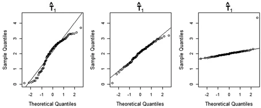
The three quantile-quantile (Q-Q) plots in Figure 4 show the sample quantiles of the maximum-likelihood estimates of
uc1(a size parameter) obtained from simulated data, plotted
making inferences about these parameters—seeNotes on our method and results.
Drosophila DNA sequence data
Maximum-likelihood estimation: To illustrate our method,
we apply it to a real, multilocus data set from two closely related species of Drosophila: Drosophila simulans and D. mela-nogaster. The DNA sequence data of Wang and Hey (2010) consist of two subsets: a large subset, which we will call the “Wang subset,” containing 30,247 blocks of intergenic se-quence; and a smaller subset, which we will refer to as the “Hutter subset,” consisting of 378 blocks of intergenic se-quence. Loci in the Wang subset were sampled by Wang and Hey (2010) from a genome alignment of four inbred lines, two fromD. simulans, and one from each ofD. melanogasterand
D. yakuba. To take into account the assumption of no recom-bination within loci and free recomrecom-bination between loci, and based on thefindings of Hey and Nielsen (2004) regarding the density of apparent recombination events inDrosophila, Wang and Hey (2010) chose a locus length of500 bp and a space of at least 2000 bp between loci. To build the Hutter subset, they drew 378 pairs ofD. melanogastersequences from the data set of Hutter et al.(2007), which consists of 378 blocks of se-quence sampled from 24 inbred lines ofD. melanogaster, with an average locus length of 536 bp and an average distance of
52 kb between consecutive loci. They then joined each of these sequence pairs with their respectiveD. yakubaorthologs from the simulans-melanogaster-yakuba genome alignment. Our models arefitted to theD. melanogasterandD. simulans
sequences from both subsets. The D. yakuba sequences are only used as outgroup sequences, to estimate the relative mu-tation rates at the different loci and to calibrate time.
Since our method uses only one pair of sequences at each of a large number of independent loci, and requires observations for all initial states, the following procedure was adopted to select a suitable set of data. According to the genome assembly they stem from, sequences in the Wang subset were given one of three possible tags:“Dsim1,” “Dsim2,”or“Dmel.”To each of the 30,247 loci in the Wang subset, we assigned a letter: loci with positions 1, 4, 7,. . .in the genome alignment were assigned the letter A; loci with positions 2, 5, 8,. . .were assigned the letter B; and loci with positions 3, 6, 9,. . .were assigned the letter C. A data set was then built by selecting observations correspond-ing to initial states 1 and 3 from the Wang subset (we used the Dsim1-Dsim2 sequences from loci A, the Dmel-Dsim1 se-quences from loci B, and the Dmel-Dsim2 sese-quences from loci C), while observations corresponding to initial state 2 were obtained from the Hutter subset by comparing the twoD. melanogastersequences available at each locus.
To estimate the relative mutation ratesrji;we use thead hoc approach proposed by Yang (2002), which was also used in Wang and Hey (2010) and Lohseet al.(2011). Estimates are
Figure 3 Estimates of migration rates and time parameters for simulated data. For each parameter, the estimates shown on the left, center, and right-hand-side boxplots are based on sample sizes of 8000, 40,000, and 800,000 loci, respec-tively. The values stated in parentheses are the true parameter values used to generate the data. Horizontal dashed lines indicate the true parameter values for each group of boxplots.
computed by means of the following method-of-moments estimator:
^ rji¼
Jkji P3
m¼1 PJm
n¼1knm
; (14)
whereJis the total number of loci, andkjiis the average of the numbers of nucleotide differences observed in pairs of one ingroup sequence and one outgroup sequence, at locusji:
Table 1 contains the maximum-likelihood estimates for the models shown in Figure 7. Note that the parameters of time and population size have been reparameterized as in Simulated data, and recall thatM1andM2are the scaled migration rates backward in time. In the diagrams, the left and right subpopu-lations representD. simulansandD. melanogaster, respectively.
Model selection:In this section, we use a series of
likelihood-ratio tests for nested models to determine which of the models
listed in Table 1fits the data of Wang and Hey (2010) best. The use of such tests in the present situation is not entirely straightforward. We wish to apply a standard large-sample theoretical result which states that, as the number of obser-vations increases, the distribution of the likelihood-ratio test statistic given by
D¼ 22log lðsÞ; where
lðsÞ ¼
sup f2F0
Lðf;sÞ
sup f2FLðf;sÞ
; (15)
approaches ax2 distribution. In Equation 15,F
0 denotes the parameter space according to the null hypothesisðH0Þ: This space is a proper subspace ofF;the parameter space
Figure 5 Q-Q plots of maximum-likelihood estimates of the parameterT1 obtained from simulated data, against the theoretical quantiles of the
standard normal distribution. The estimates shown in the left-hand-side, center, and right-hand-side Q-Q plots are based on sample sizes of 8000, 40,000, and 800,000 loci, respectively.
Figure 4 Q-Q plots of maximum-likelihood estimates of the parameteruc1 obtained from simulated data, against the theoretical quantiles of the
according to the alternative hypothesisðH1Þ:The number of degrees of freedom of the limiting distribution is given by the difference between the dimensions of the two spaces. A list of sufficient regularity conditions for this result can be found, for example, in Casella and Berger (2001, p. 516). One of them is clearly not met in the present case: in the pairwise comparison of some of our models, every point ofF0is a boundary point of F:In other words, ifH0is true, the vector of true parameters
f*2F0;whichever it might be, is on the boundary ofF:This irregularity is present, for example, when M1¼M2¼0 according toH0 andM1;M22 ½0;NÞ according toH1:The problem of parameters on the boundary has been the subject of articles such as Self and Liang (1987) and Kopylev and Sinha (2011). The limiting distribution of the likelihood-ratio test statistic under this irregularity has been derived in these articles, but only for very specific cases. In most of these cases, the use of the naivex2
rdistribution, withrbeing the number of
additional free parameters according to H1;turns out to be conservative, because the correct null distribution is a mixture ofx2
ndistributions withn#r:Our analysis of the data of Wang and Hey (2010) involves two likelihood-ratio tests with pa-rameters on the boundary (ISOvs.IM1, and IM1vs.IIM1), so we need to check that the naivex2
rdistribution is also
conser-vative in these cases. This was verified in a short simulation study which we now describe.
We generated 100 data sets from the ISO model, each one consisting of 40,000 observations, and fitted both the ISO model ðH0Þand the IM1modelðH1Þ to obtain a sample of
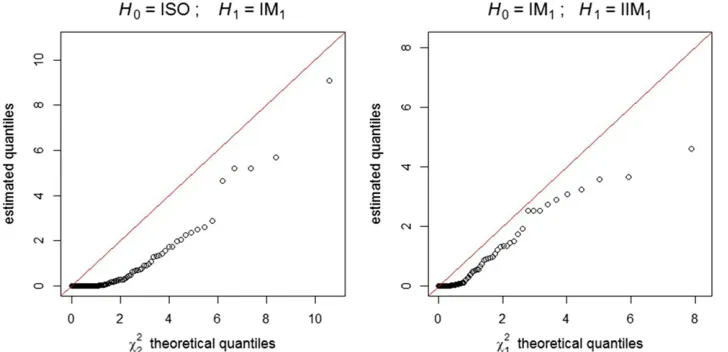
100 realizations of the likelihood-ratio test statistic. A Q-Q plot (Figure 8, left boxplot) shows that the estimated quan-tiles of the null distribution are smaller than the correspond-ing theoretical quantiles of the x2 distribution with two degrees of freedom (the difference between the dimensions ofF0andFin this particular case). In other words, the use of the naivex2distribution is conservative in this case. Usingx2 2 instead of the correct null distribution, at a significance level of 5%, the null hypothesis (i.e., the ISO model) was falsely rejected in only 1 out of the 100 simulations performed.
A similar simulation was carried out with respect to another pair of nested models: the IM1model (now asH0), in which
t1¼0;and the IIM1modelðH1Þ;in whicht1.0:Again, the naivex2distribution (this time with only one degree of free-dom) was found to be conservative (Figure 8, right boxplot). And once more, only in 1 out of the 100 simulations per-formed is the null hypothesis (the IM1model) falsely rejected at the 5% significance level, ifx2
1is used instead of the correct null distribution.
To select the model that bestfitted the data of Wang and Hey (2010), we performed the sequence of pairwise compar-isons shown in Table 2. For any sensible significance level, this sequence of comparisons leads to the choice of IIM2as the best-fitting model. In fact, assuming the naivex2as the null distribution, a significance level as low as 1:2310274is enough to rejectH0in each of the three tests. However, since
^
M1¼0 for this model (see Table 1), afinal (backward) com-parison is in order: one between IIM2 and IIM3 (which
Table 1 Maximum-likelihood estimates and values of the maximized log-likelihood
Model ua u ub uc1 uc2 T1 V M1 M2 logLðfÞ
ISO 4.757 5.628 2.665 — — — 13.705 — — 290,879.14
IM1 3.974 5.641 2.493 — — — 14.965 0.000 0.053 290,276.00
IIM1 3.191 5.581 2.589 — — 6.931 9.928 0.000 0.528 290,069.44
IIM2 3.273 3.357 1.929 6.623 2.647 6.930 9.778 0.000 0.223 289,899.22
IIM3 3.273 3.357 1.929 6.623 2.647 6.930 9.778 — 0.223 289,899.22
Results for the data of Wang and Hey (2010), for the models shown in Figure 7.
Figure 6 Q-Q plots of maximum-likelihood estimates of the parameterM1obtained from simulated data, against the theoretical quantiles of the
corresponds tofixingM1at zero in IIM2). The nested model in this comparison has one parameter less and, as can be seen in Table 1, has the same likelihood. So, in the end, we should prefer IIM3to IIM2.
Confidence intervals for the selected model: The Wald
confidence intervals are straightforward to calculate when-ever the vector of estimates is neither on the boundary of the model’s parameter space, nor too close to it. In that case, it is reasonable to assume that the vector oftrueparameters does not lie on the boundary either. As a consequence, the vector of maximum-likelihood estimators is consistent and its distribu-tion will approach a multivariate Gaussian distribudistribu-tion as the sample size grows (see, for example, Pawitan 2001, p. 258). The confidence intervals can then be calculated using the inverted Hessian matrix.
In the case of the data of Wang and Hey (2010), the vector of estimates of the selected model (IIM3) is an interior point of the parameter space. Assuming that the vector of true parameters is also away from the boundary, we computed the Wald 95% confidence intervals shown in Table 3 using
the inverted Hessian. In agreement with our assumption, we note that none of the confidence intervals include zero.
For large sample sizes, and for true parameter values not too close to the boundary of the parameter space, the Wald intervals are both accurate and easy to compute. To check how well the Wald intervals for the IIM3model fare against the more accurate (see Pawitan 2001, pp. 47–48), but also com-putationally more expensive, profile likelihood intervals, we included these in Table 3. The two methods yield very similar confidence intervals for all parameters exceptub:The cause
of this discrepancy should lie in the fact that we only had pairs ofD. melanogastersequences available from a few hun-dred lociðubis the size of theD. melanogastersubpopulation
during the migration stage).
Conversion of estimates:The conversion of point estimates
and confidence intervals to more conventional units is based on the estimates of Powell (1997) of the duration of one generationðg¼0:1 yearsÞand the speciation time between
D. yakuba and the common ancestor of D. simulans and
D. melanogaster (10 MY); see also Wang and Hey (2010)
Figure 8 Q-Q plots of the estimated quantiles of the likelihood-ratio test sta-tistic null distribution against thex2
dis-tribution theoretical quantiles. Left plot:
H0= ISO model,H1= IM1model. Right
plot: H0 = IM1 model, H1 = IIM1
model.
Figure 7 Models fitted to the data of Wang and Hey (2010): ua¼ua; ub¼ub; uc1¼uc1; uc2¼uc2;
and Lohseet al.(2011). Using these values, we estimatedm, the mutation rate per locus per generation, averaged over all loci, to bem^¼2:3131027:
In Table 4, Table 5, and Table 6, we show the converted estimates for the best-fitting model IIM3. The effective pop-ulation size estimates, in units of diploid individuals, are all based on estimators of the formNb ¼ ð1=4m^Þ3^u:For exam-ple, the estimate of the ancestral population effective sizeNa
is given by ð1=4m^Þ3^ua:The estimates in years of the time
since the onset of speciation and of the time since the end of gene flow are given by ^t0¼ ðg=2m^Þ3ðTb1þVbÞ and
^t1¼ ðg=2m^Þ3bT1; respectively. With respect to gene flow, we use^q1¼m^3ðMb2^b=^uÞas the estimator of thefractionof subpopulation 1 that migrates to subpopulation 2 in each generation, forward in time; and^s1¼ ðMb2^b=2Þas the estima-tor of thenumberof migrant sequences from subpopulation 1 to subpopulation 2 in each generation, also forward in time. Ifgandm^ are treated as constants, then each of the esti-mators just given can be expressed as a constant times a product—or a ratio—of the estimators of nonconverted pa-rameters. For example, we have that
^ q1¼m^3
^ Mb2^b
^
u ¼constant3
^ Mb2^b
^
u ;
and
N
ba¼
^
ua
4m^¼constant3^ua:
Suppose the IIM3model is reparameterized in terms of
f¼ ðua u ub uc1 uc2 T1 T1þV M2b=uÞ
T;
andf^denotes the maximum-likelihood estimator off:Then the estimatorf^cof the vector of converted parameters
fc¼ ðNa N Nb Nc1 Nc2 t1 t0 q1Þ
T;
can be written asf^c¼Wf^;whereWis a diagonal matrix. The random vector f^ is a maximum-likelihood estimator (of a reparameterized model). Hence, for a large enough sample size, its distribution is approximately multivariate Gaussian, with some covariance matrix∑;and the distribution off^cis approximately multivariate Gaussian with covariance matrix
W∑WT:To calculate the Wald confidence intervals of Table 4,
Table 5, and Table 6, we used the inverse of the observed Fisher information as an estimate of∑:An estimate ofW∑WT followed trivially.
Profile likelihood confidence intervals were also computed for the parameterization f¼ ðua ;. . .; M2b=uÞT:Then, if ^u
ðor^lÞ is the vector of estimated upper (or lower) bounds for the parameters in f; W^u ðorW^lÞ will be the vector of estimated upper (or lower) bounds for the converted param-eters. This follows from the likelihood-ratio invariance—see, for example, Pawitan (2001, pp. 47–48). Confidence inter-vals for the converted migration parameters1(rather thanq1 in the procedure above) were obtained analogously, using a slightly different reparameterization of the IIM3model.
Discussion
Notes on our method and results
We have described a fast method tofit the IIM model to large data sets of pairwise differences at a large number of in-dependent loci. This method relies essentially on the eigen-decomposition of the generator matrix of the process during the migration stage of the model: for each set of parameter values, the computation of the likelihood involves this de-composition. Nevertheless, the whole process of estimation takes no more than a couple of minutes for a data set of tens of thousands of loci such as that of Wang and Hey (2010), and it does not require high-performance computing resources. The implementation of the simpler IIM model of Wilkinson-Herbots (2012), with R code provided in Wilkinson-Wilkinson-Herbots (2015), is even faster than the more general method pre-sented here, since it makes use of a fully analytical expression for the likelihood (avoiding the need for eigen-decomposi-tion of the generator matrix); but it relies on two assumpeigen-decomposi-tions which we have dropped here, and which are typically unre-alistic for real species: the symmetry of migration rates and the equality of subpopulation sizes during the gene flow period.
Due to the number of parameters, it is not feasible to assess the performance of our method systematically over every region of the parameter space. However, our experience with simulated data sets suggests that there are two cases in which the variances of some estimators become inflated, in partic-ular the variances of the estimators associated with the gene
flow periodðMb1;Mb2;u^;^ub;andVbÞ:One of such cases arises Table 3 Point estimates and confidence intervals under the model IIM3
Parameter Estimate
95% confidence intervals
Wald Profile likelihood
ua 3.273 (3.101, 3.445) (3.100, 3.444)
u 3.357 (3.139, 3.575) (3.097, 3.578)
ub 1.929 (0.079, 3.779) (0.672, 5.010)
uc1 6.623 (6.407, 6.839) (6.415, 6.843)
uc2 2.647 (2.304, 2.990) (2.331, 3.021)
T1 6.930 (6.540, 7.320) (6.542, 7.319)
V 9.778 (9.457, 10.099) (9.456, 10.098)
M2 0.223 (0.190, 0.256) (0.186, 0.259)
Results refer to the data of Wang and Hey (2010). Table 2 Forward selection of the best model
H0 H1 22loglðSÞ P-value
ISO IM1 603.14 1.147E2262
IM1 IIM1 413.12 7.673E292
IIM1 IIM2 340.44 1.187E274
wheneverVis very small orT1is very large, making it very unlikely that the genealogy of a pair of sequences under the IIM model is affected by events that occurred during the gene
flow period. The second case arises when the values of the scaled migration rates are greater than one, so that the two subpopulations during the period of gene flow resemble a single panmictic population. In either of these cases, the very process of model fitting can become unstable, that is, the algorithm of maximization of the likelihood may have diffi -culty converging.
Problems can also arise if the number of loci is insufficient. The simulation study in theSimulated datasection suggests that convergence to sensible parameter estimates is still pos-sible for a sample size of 8000 loci. However, when wefitted the full IIM model to a simulated sample of 4000 loci (results not shown), outliers started to emerge. It should also be noted that for sample sizes of just a few thousand loci, the distribution of migration rate estimates is still far from Gauss-ian (Figure 6). In such cases, computation of confidence in-tervals should be based on bootstrap methods or on the likelihood (profile likelihood confidence intervals) rather than on the Hessian (Wald confidence intervals). How many loci are needed to obtain good estimates and confidence in-tervals will also depend on the region of the parameter space concerned.
It is not the goal of this article to draw conclusions re-garding the evolutionary history of Drosophilaspecies. We used the data of Wang and Hey (2010) with the sole objective of demonstrating that our method can be applied efficiently and accurately to real data. In Table 7, we list both our esti-mates and those of Wang and Hey (2010) for a six-parameter isolation-with-migration model (the IM1model—see Figure 7). The same table contains the estimates for our best-fitting IIM model. Our parameter estimates for the IM model agree well with those of Wang and Hey (2010). The reason that they do not match exactly lies in the fact that we have omitted the “screening procedure”described in Wang and Hey
(2010) and have therefore not excluded some of the most divergent sequences in the data set. It should also be borne in mind that our model of mutation is the infinite-sites model, whereas Wang and Hey (2010) have worked with the Jukes– Cantor model. Furthermore, our choice of sequence pairs was somewhat different: Wang and Hey (2010) randomly se-lected a pair of sequences at each locus, whereas we followed the procedure described in the Maximum-likelihood estima-tionsection.
There are some otable differences between the estimates for both IM models and those for the IIM model: under the IIM model, the process of speciation is estimated to have started earlier (3.6 MYA instead of 3.0 or 3.2 MYA), to have reached complete isolation before the present time (1.5 MYA), and to have a higher rate of geneflow (0.064 sequences per gener-ation instead of 0.013 or 0.012 sequences) during a shorter period of time (2.1 MY of geneflow instead of 3.0 or 3.2 MY). As might be expected, the estimates of each descendant population size (D. simulansandD. melanogaster) in the IM models lie in between the estimates of the corresponding current population size and its size during the gene flow period in the IIM model.
The method we used assumes that relative mutation rates are known (see The likelihood of a multilocus data set). In reality, we must deal with estimates of these rates, and this introduces additional uncertainty which is not reflected in the standard errors and confidence intervals obtained. In principle, this uncertainty can be reduced by increasing the number of ingroup and outgroup sequences used to compute the average number of pairwise differences at each locus in Equation 14. Ideally, estimates of the relative mutation rates should be based on outgroup species only (Wang and Hey 2010) to avoid any dependence between the estimates of relative mutation rates and the observations on ingroup pair-wise differences, but this was not possible here since the Wang and Hey (2010) data included exactly one outgroup sequence for each locus.
Table 5 Divergence time estimates under the model IIM3
Event Time since occurrence
95% confidence intervals
Wald Profile likelihood
Onset of speciationðt0Þ 3.624 (3.559, 3.689) (3.561, 3.691)
Complete isolationðt1Þ 1.503 (1.419, 1.588) (1.419, 1.587)
Divergence time estimates for the data of Wang and Hey (2010), given in millions of years ago. Values shown are the converted estimates oft0andt1(see Figure 1). Table 4 Effective population size estimates under the model IIM3
Population Population size
95% confidence intervals
Wald Profile likelihood
Ancestral populationðNaÞ 3.549 (3.362, 3.736) (3.362, 3.735)
D. simulans, migration stage (N) 3.640 (3.404, 3.877) (3.359, 3.880)
D. melanogaster, migration stageðNbÞ 2.092 (0.085, 4.099) (0.729, 5.433) D. simulans, isolation stageðNc1Þ 7.182 (6.949, 7.415) (6.957, 7.421)
D. melanogaster, isolation stageðNc2Þ 2.871 (2.498, 3.243) (2.528, 3.276)
Violation of assumptions
Some assumptions of the IIM model in this article, such as the infinite-sites assumption and the assumption of free recom-bination between loci and no recomrecom-bination within loci, may not be sensible for some real data sets. The appropriateness of other assumptions, for example those regarding the constant size of populations or the constant rate of gene flow, will depend on the actual evolutionary history of the species or populations involved. While a systematic, in-depth robustness analysis of our method (similar to, for example, the robustness studies by Becquet and Przeworski 2009 and Strasburg and Rieseberg 2010 for commonly used IM methods) is beyond the scope of this article, we will in this section informally examine the impact of possible violations of some of the main assumptions made.
Misspecification of the demographic model:To explore the
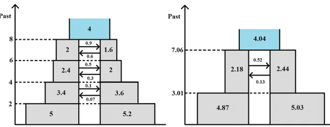
potential effect of misspecification of the demographic model on inference accuracy, we first simulated 20 data sets of 40,000 loci each from a somewhat more complex evolutionary scenario, depicted in the left-hand side diagram of Figure 9, where subpopulation sizes gradually increase and geneflow gradually declines. The precise parameter values assumed for the true model were chosen arbitrarily and are shown in the left-hand side diagram; in accordance with the reparamete-rization used in Simulated data, divergence times are mea-sured on a mutational scale by twice the expected number of mutations per sequence (as an average over all loci), popu-lation sizes are represented by scaled mutation rates, and rates of geneflow by scaled migration rates. We then applied our method tofit isolation, IM, and IIM models to each of the simulated data sets and selected the best-fitting model by
means of likelihood-ratio tests—for each of the 20 data sets generated this was found to be the full IIM model. The aver-age point estimates obtained for each parameter are shown on the right-hand-side diagram of Figure 9. In each diagram, the widths of the boxes are proportional to the population sizes and the heights are proportional to the durations of the time periods concerned. It is readily seen that the IIM model reflects the dynamics of the true model quite well. Population sizes, migration rates, and splitting times are all estimated at intermediate values.
We also repeated the simulation and estimation procedure for an evolutionary scenario involving a period of secondary geneflow, depicted in the left-hand side diagram of Figure 10. Again, for each of the 20 simulated data sets, the full IIM model provides the best fit among the models considered (isolation, IM, and IIM). Comparing the two diagrams in Figure 10 (where the IIM parameter values in the right-hand-side diagram are again the averages of the estimates obtained for the 20 simulated data sets), we see that the IIM model obtained provides a reasonable approximation to the true model, though of course our method did not detect the initial period of isolation as this feature was not included in the set of modelsfitted. The estimates of the time since the onset of speciation and the time since complete isolation are, on average, close to the true values in this case. The average estimates of the migration rate and population size parame-ters are again at intermediate values, compared to the range of true values over time.
Intralocus recombination:In common with other methods
mentioned in this article (for example, Wang and Hey 2010; Lohse et al. 2011), our method assumes that there is no
Table 7 Comparison of converted estimates obtained with IM and IIM models
IMwh IM1 IIM3
Time since onset of speciation 3.040 3.240 3.624
Time since isolation — — 1.503
Size of ancestral population 3.060 4.310 3.549
Current size ofD. simulanspopulation 5.990 6.120 7.182
Current size ofD. melanogasterpopulation 2.440 2.700 2.871
Size ofD. simulanspopulation during IIM geneflow period — — 3.640
Size ofD. melanogasterpopulation during IIM geneflow period — — 2.092
Migration rate (D. simulans/D. melanogaster) 0.013 0.012 0.064
Migration rate (D. melanogaster/D. simulans) 0.000 0.000 —
Times are given in millions of years; population sizes are given in millions of individuals; the migration rates stated represent the number of sequences that migrate per generation, forward in time. The model IMwhis the IM modelfitted by Wang and Hey (2010).
Table 6 Converted migration rates under the model IIM3
Migration parameter Point estimate
95% confidence intervals
Wald Profile likelihood
Migration rateðq1Þ 8.8E209 (1.1E-10, 1.8E208) (3.2E209, 2.4E208)
Number of migrant sequencesðs1Þ 0.064 (0.001, 0.127) (0.023, 0.172)
Converted migration rates for the data of Wang and Hey (2010). Values shown refer to forward-in-time parameters:q1is the fraction of subpopulation 1 (D. simulans) that
migrates to subpopulation 2 (D. melanogaster) in each generation, during the period of geneflow;s1is the number of sequences migrating from subpopulation 1 to
recombination within loci and free recombination between loci. Thefirst of these two assumptions is the most important one, without which our method would not be valid. Recom-bination within loci mixes up the genealogies of DNA se-quences on which our method relies, making pairs of sequences more equidistant: intralocus recombination does not affect the mean number of segregating sites in a pair of sequences but thevariancedecreases with increasing recom-bination (Griffiths 1981; Hudson 1983; Schierup and Hein 2000), resulting in data sets which contain more intermedi-ate values and fewer extreme values. This can be expected to lead to overestimation of the current population sizes and underestimation of the ancestral population size, while the effect on estimates of the other parameters is intuitively somewhat less obvious. The impact of intralocus recombina-tion on the variance of the number of pairwise differences, and hence on the accuracy of our method, may be expected to be less severe in cases of recombination rate heterogeneity within loci (seefigure 1 in Hudson 1983, for the extreme case of recombination hotspots separating completely linked regions).
A simulation study by Strasburg and Rieseberg (2010) found that even relatively low levels of intralocus recombi-nation can cause substantial bias in estimates of the IM model parameters obtained using the programIMa(Hey and Nielsen 2007), with highest posterior density intervals failing to contain the true parameter values far more often than would be expected by chance. In IM simulations allowing a minimal but realistic amount of intralocus recombination, Lohseet al.
(2016) found that the bias in their parameter estimates was small. Although our method and model are different from those of Hey and Nielsen (2007) and Lohse et al. (2016),
the effect of recombination on the underlying genealogies remains the same, and therefore similar biases will occur if the assumption of no intralocus recombination is violated.
For theDrosophiladata considered in this article, Wang and Hey (2010) assessed the impact of potential intralocus recombination on their estimates of the parameters of an IM model by comparison with the estimates obtained from the same sequences but halved in length (i.e., approximately halving the expected number of intralocus recombination events). Their estimates of the ancestral population size and the migration rate from the half-length data were
30% larger than those from the full-length data, while the differences for the other parameter estimates were small. In the same spirit, we repeated our previous analysis of the
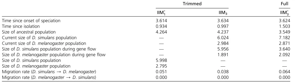
Drosophiladata but now using the trimmed version of the Wang subset prepared by Lohse et al. (2011), in which the average locus length was reduced by approximately a factor of 3; the Hutter subset (1% of the total number of loci) was retained in its entirety as we could not afford to further reduce this already very small data set of D. mela-nogasterpairs. Applying the estimation and model selection procedures described inDrosophila DNA sequence datato this trimmed version of the data, the likelihood-ratio test of the models IIM1vs.IIM2was no longer significant,i.e., there was no longer significant evidence of an increase in population size at time T1; and the best-fitting model was a unidirec-tional version of IIM1(i.e., withM1¼0Þ:
Table 8 shows the estimates obtained from the trimmed data; the estimates obtained earlier in this article from the full data are also listed again for comparison. In line with our expectations regarding the potential effect of intralocus re-combination, it is seen that the full data gave a larger
Figure 10 Violation of demographic assump-tions. Left-hand-side diagram: true model. Right-hand-side diagram: best-fitting IIM model. Divergence times are measured by twice the expected number of mutations per sequence, population sizes are represented by scaled mu-tation rates, and rates of geneflow by scaled migration rates.
estimate of the current population size ofD. simulansand a smaller estimate of the ancestral population size; the esti-mated size ofD. simulansduring the geneflow stage was also smaller than that obtained from the trimmed data. The esti-mated time since the onset of speciation is nearly identical for the two data sets, but the full data placed the end of geneflow substantially further back into the past (1.5 MYA compared to 0.93 MYA) and estimated a somewhat higher number of migrant sequences per generation (0.064 compared to 0.051) during a shorter period of geneflow (2.12 MY com-pared to 2.68 MY). This suggests that, in addition to the impact on population size estimates already discussed, intra-locus recombination may lead to an overestimate of the time since the end of geneflow in an IIM model and (possibly as a consequence) an overestimate of the migration rate. Never-theless, for both versions of theDrosophiladata, the likeli-hood-ratio tests of nonzero migration rate and nonzero time since the end of geneflow were significant.
The above considerations imply that, when preparing data for use with our method (or any other method relying on the assumption of no intralocus recombination), loci should be chosen carefully to try to keep the amount of intralocus recombination negligible, and some caution may be needed in the interpretation of results. For data sets showing signs of recombination within loci, it may be possible to reduce its effect by trimming or breaking up such loci to form shorter, apparently nonrecombining segments of DNA sequence (Hey and Nielsen 2004; Strasburg and Rieseberg 2010). An exten-sion of our method to account for recombination within loci would be of interest but is challenging. An extension to a
finite-sites model for use with shorter fragments of DNA se-quence would also be of interest—such an extension is rela-tively straightforward but is yet to be implemented in our method (but see Wang and Hey 2010 and Andersen et al.
2014 for the IM model).
Linkage disequilibrium: If the assumption of free
recombi-nation between loci does not hold, then loci are not indepen-dent, in which case the likelihood in Equation 13 is in fact a
composite marginal likelihood (also called the“independence likelihood”in Chandler and Bate 2007) rather than an ordi-nary full likelihood (see Varin 2008 for an overview of com-posite marginal likelihood methods; see also the discussion of Lohse et al. 2016). Statistical theory indicates that in that case, the maximum composite likelihood estimator (MCLE) is still consistent (Cox and Reid 2004; Wiuf 2006, with some minor modifications to account for our slightly different assumptions; Varin 2008), provided the relative mutation rates at the different loci are bounded. Thus, if linkage be-tween loci cannot be ignored, the MCLE of the parameters of the IIM model obtained with our method will still be approx-imately unbiased if the number of loci is sufficiently large, and if all our other assumptions hold (including the assump-tion of no recombinaassump-tion within loci). However, if linkage between loci is not negligible, then standard errors and confidence intervals computed using the observed Fisher information (as was done in theResultssection) will un-derestimate the true uncertainty about the parameter esti-mates obtained (Baird 2015); instead, standard errors and confidence intervals should be based on an estimate of the Godambe information (Godambe 1960). For a data set made up of a single string of correlated loci, or a small number of such strings, obtaining an accurate estimate of the Godambe information presents some difficulties (see Varin 2008 and Varinet al. 2011 for a discussion and some possible strate-gies). A much simpler situation arises if the data consist of a sufficiently large number of “clusters” of loci, where loci within clusters are correlated but where different clusters can be considered independent. This may be the case, for example, if different clusters of loci are chosen from different chromosomes, or are separated by recombination hotspots or by a large enough distance along the genome. For such data, an empirical estimate of the Godambe information can easily be computed as described in Chandler and Bate (2007) or Varin (2008).
To try to quantify the effect of linkage on the standard errors of the IIM parameter estimates, we conducted the following analysis of a suitable subset of the Wang and Hey
Table 8 Converted estimates for full sequences and trimmed sequences
Trimmed Full
IIM*
1 IIM3 IIM*3
Time since onset of speciation 3.614 3.634 3.624
Time since isolation 0.934 0.997 1.503
Size of ancestral population 4.264 4.237 3.549
Current size ofD. simulanspopulation — 6.024 7.182
Current size ofD. melanogasterpopulation — 2.984 2.871
Size ofD. simulanspopulation during geneflow — 5.956 3.640
Size ofD. melanogasterpopulation during geneflow — 1.891 2.092
Size ofD. simulanspopulation 5.998 — —
Size ofD. melanogasterpopulation 2.795 — —
Migration rate (D. simulans/D. melanogaster) 0.051 0.038 0.064
Migration rate (D. melanogaster/D.simulans) 0.000 0.000 0.000