Identification of Statistical Energy Analysis Parameters from Measured Data

ABSTRACT

GREGORY, JOSEPH WILLIAM. Identification of Statistical Energy Analysis Parameters from Measured Data. (Under the Direction of Dr. Richard F. Keltie)

An approach for identifying statistical energy analysis (SEA) parameters from experimental investigation is presented. Specifically, a power flow realization method (PRM) and

statistical energy analysis model improvement (SMI) technique using transient time-domain vibration measurements are derived. The efforts are refined and validated using a range of test simulations, and then with true physical tests conducted on both simple and complex structures. Experimentation is also used to define the necessary input power measurements, response energy measurements, and data processing techniques necessary for successful PRM/SMI.

It is found that utilization of time domain data allows for an over-determined power balance providing favorable numerical conditions for the identification. In fact, it is observed that a full matrix of measured inputs and outputs is not necessarily required for successful

IDENTIFICATION OF STATISTICAL ENERGY ANALYSIS

PARAMETERS FROM MEASURED DATA

By

JOSEPH WILLIAM GREGORY

A thesis submitted to the Graduate Faculty of North Carolina State University

in partial fulfillment of the requirements for the Degree of

Doctor of Philosophy

DEPARTMENT OF MECHANICAL AND AEROSPACE ENGINEERING

Raleigh

2002

APPROVED BY:

________________________________ ________________________________ Dr. Harvey Johnson Charlton Dr. Charles E. Hall, Jr.

________________________________ ________________________________ Dr. Robert T. Nagel Dr. Richard F. Keltie

BIOGRAPHY

ACKNOWLEDGEMENTS

The author acknowledges the primary sponsor of this work, the National Science Foundation under Grant No. CMS-9908326. Sincere thanks are given to Vibro-Acoustic Sciences, Inc. for use of their software, Ford Motor Company for their generous donation of a vehicle used as a test-bed in this effort, and the NASA Langley Research Center for use of the system identification software, SOCIT.

Grateful acknowledgment is given to Dr. Richard F. Keltie who has come to be the author’s mentor, friend, and inspiration to pursue research challenges. Gratitude is also extended to the members of the advisory committee: Dr. Harvey Johnson Charlton, Dr. Charles E. Hall Jr., and Dr. Robert T. Nagel.

TABLE OF CONTENTS

List of Tables

vii

List of Figures

viii

1

Introduction

1

1.1 Background 1

1.1.1 Structural Dynamics 1

1.1.2 Analysis Methods 6

1.1.3 Conclusions 10

1.2 Predictive SEA 12

1.2.1 History 12

1.2.2 Coupled Systems 12

1.2.3 Power Balance 18

1.2.4 Conclusions 24

1.3 SEA Model Development 25

1.3.1 Modal Density 26

1.3.2 Damping Loss Factor 28

1.3.3 Coupling Loss Factor 30

1.3.4 Summary 32

1.4 Experimental SEA 34

1.4.1 Classical Power Injection Method 35

1.4.2 Improved Power Injection Method 36

1.4.3 Normalized Energy Inversion Method 38

1.5 Conclusions 41

2

Development of a Power Flow Model Realization Method

42

2.1 Problem Definition and Approach 42

2.2 Selection of System Identification Method 45

2.3 State Space Realization 50

2.3.1 Quasi-Steady State Sea 50

2.3.2 Transform Theory and State Space Representation 53

2.3.3 System Realization 59

2.3.4 Response Synthesis and Test/Analysis Correlation 71

3

Development of a SEA Model Improvement Procedure

75

3.1 Approach 75

3.2 Eigenvector Inversion 77

3.2.1 Non-Symmetric System 77

3.2.2 Symmetric System 79

3.3 Expansion of Unmeasured Degrees Of Freedom 84

3.4 Summary 87

4

Simulations

88

4.1 Two Subsystem Model 88

4.2 Multi-Subsystem Model 99

4.3 Conclusions 102

5

Experimental Studies

104

5.1 Simple Structure 105

5.1.1 Experimental Setup 105

5.1.2 Transient Data Pre-Processing 108

5.1.3 Realization of a Minimum Order Power Flow Model 111

5.1.4 SEA Model Improvement 112

5.1.5 Discussion of Results 116

5.1.6 Conclusions 117

5.2 Complex Structure 119

5.2.1 Experimental Setup 119

5.2.2 Pretest Analysis 121

5.2.3 System Identification and Model Improvement 127 5.2.4 Identification of Structural Change 133

5.2.5 Conclusions 136

6

Summary and Recommendations

137

LIST OF TABLES

Table 1.1 Modal Densities of Idealized Systems 27

Table 1.2 Damping Measures 28

Table 2.1 Transfer Function Models 47

Table 2.2 State Space Form of the Quasi-steady State Power Balance 57

Table 4.1 Eigenvalues of Two-Subsystem Simulation 90

LIST OF FIGURES

Figure 1.1 Structural Dynamic Investigation 1

Figure 1.2 FEA Model of Spacecraft Body 3

Figure 1.3 FEA Model of Automobile Front End 3

Figure 1.4 Scale Model Test of a Propeller 5

Figure 1.5 Ground Vibration Test of F-22 Aircraft at Edwards Air Force Base 5

Figure 1.6 Coupled Oscillators 12

Figure 1.7 Coupling Coefficient 15

Figure 1.8 Coupling Coefficient Magnitude 16

Figure 1.9 Mode Pair Interactions of Coupled Dynamic Systems 16

Figure 1.10 Three Subsystem SEA Model 18

Figure 1.11 Quadratic Form of Two-Subsystem Coupling Matrix 22 Figure 1.12 Simple Structure Decomposed into SEA Subsystems 25

Figure 1.13 Measurement of Coupling Loss 31

Figure 2.1 Dynamic System with Input and Disturbance 46

Figure 2.2 Eigensystem Realization Algorithm 66

Figure 2.3 Power Flow Realization Method (PRM) 70

Figure 3.1 Structural Dynamic Model Updating 75

Figure 3.2 Power Flow Realization Method (PRM) and SEA Model Improvement

(SMI) 87

Figure 4.1 Two-Subsystem SEA Model 88

Figure 4.2 Two-Subsystem SEA Simulation 89

Figure 4.3 Decomposition of Two-Subsystem Block Correlation Matrix 90

Figure 4.4 Eigenvalue Error (Case 1) 92

Figure 4.5 Damping Loss Factor (Case 1) 93

Figure 4.6 Normalized Coupling Matrix Update (Case 1) 94

Figure 4.7 Eigenvalue Error (Case 2) 95

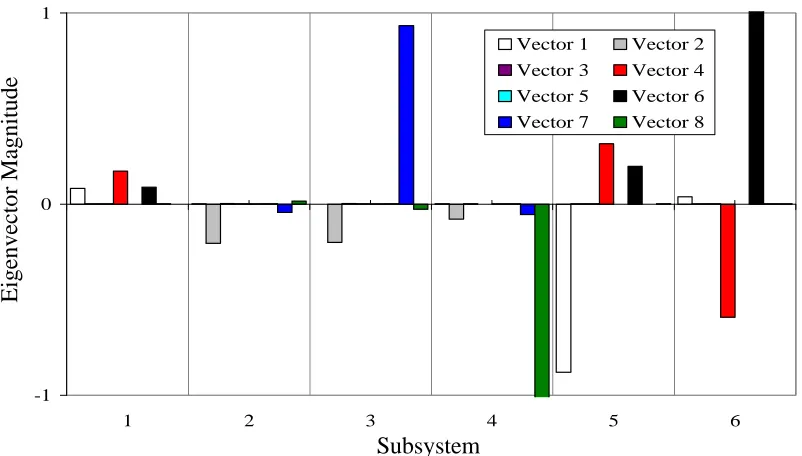
Figure 4.8 Identified Damping and Coupling Loss Factor (Case 2) 96 Figure 4.9 Subsystem 1 Damping Loss Factor (Case 2) 97 Figure 4.10 Eigenvectors of Initial Multi-Subsystem Computational SEA Model 99

Figure 4.11 SMI with Good Choice of Eigenvectors 100

Figure 4.12 SMI with Poor Choice of Eigenvectors 101

Figure 4.13 SMI with Noise and Good Choice of Eigenvectors 101 Figure 4.14 SMI with Noise and Poor Choice of Eigenvectors 102

Figure 4.15 Effect of Initial Model Inaccuracy 103

Figure 5.1 Simple Structure Test Setup 105

Figure 5.2 Damping Tile Treatment 106

Figure 5.5 Response Velocity, 1000 Hz 110

Figure 5.6 Spatial Average of Response, 1000 Hz 111

Figure 5.7 Measured and PRM Results, 1000 Hz 112

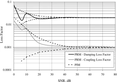
Figure 5.8 Coupling Loss Factors 113

Figure 5.9 Coupling Loss Factor Error 114

Figure 5.10 Damping Loss Factors 114

Figure 5.11 Damping Loss Factor Error 115

Figure 5.12 Drive Point Mobility of Large Plate 116

Figure 5.13 Drive Point Mobility of Small Plate 117

Figure 5.14 Transfer Mobility 117

Figure 5.15 Mercury Sable Test Setup 119

Figure 5.16 Instrument Setup 120

Figure 5.17 SEA Model of Mercury Sable Test Structure 121

Figure 5.18 Relative Activation of Eigenpairs 123

Figure 5.19 Total System Activation, 1000 Hz 124

Figure 5.20 Total System Activation 124

Figure 5.21 Thermogram of Frequency Average Activation (Plates) 125 Figure 5.22 Thermogram of Frequency Average Activation (Beams) 126

Figure 5.23 Location of Drive Point Excitation 126

Figure 5.24 Measured Beam Response Locations 127

Figure 5.25 Eigenvector Participation at Test Locations 128

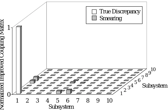
Figure 5.26 Change in Coupling Matrix, 1000 Hz 129

Figure 5.27 Locations of Initial Model Coupling Loss Factor Errors, 1000 Hz 130

Figure 5.28 Result of SEA Model Improvement 131

Figure 5.29 Drive Point Mobility 132

Figure 5.30 Roof Trans fer Mobility 132

Figure 5.31 Windshield Transfer Mobility 133

Figure 5.32 Normalized Coupling Matrix Update 134

1 INTRODUCTION

1.1 BACKGROUND

1.1.1 STRUCTURAL DYNAMICS

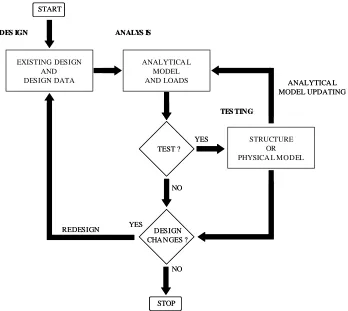
The subject of structural dynamics involves the study of the response of structures due to dynamic loading. Over the last sixty years, structural dynamic analysis and testing has been successfully incorporated into many engineering efforts including the design of aircraft, spacecraft, automobiles, surface ships, submarines, bridges, dams, buildings, and many others. There are typically three phases involved with a structural dynamic investigation as diagrammed in Figure 1.1. These are: design, analysis, and testing. More recently,

additional consideration is sometimes given to the evaluation of control strategies and to the use of a concurrent rather than sequential approach to the investigation.

Figure 1.1 Structural Dynamic Investigation

ANALYS IS

REDESIGN

NO

YES START

NO EXISTING DESIGN

AND DESIGN DATA

ANALYTICA L MODEL AND LOADS

TEST ?

DESIGN CHANGES ?

STRUCTURE OR PHYSICA L MODEL

DES IGN

TESTING

YES

ANALYTICA L MODEL UPDATING

STOP

ANALYS IS

REDESIGN

NO

YES START

NO EXISTING DESIGN

AND DESIGN DATA

ANALYTICA L MODEL AND LOADS

TEST ?

DESIGN CHANGES ?

STRUCTURE OR PHYSICA L MODEL

DES IGN

TESTING

YES

ANALYTICA L MODEL UPDATING

Often, there exist design problems that require a structural dynamic investigation to be linked to an associated structural acoustic study. In these situations, the interaction between

structural motion and a connected acoustic field is a key consideration. As a result, the frequency range of interest may be very wide and, in fact, may include the entire bandwidth of human hearing, 20 Hz – 20,000 Hz. Current analysis techniques are applicable only in certain frequency ranges such that assumptions associated with the specific approach are satisfied. As a result, it is usually necessary to divide the analysis into three parts: the low frequency region, the middle frequency region, and the high frequency region. Note, a strict boundary between the regions does not exist and depends, more specifically, on the number of modes that exist in the range of the analysis applied as well as the ratio of the size of the structure to the wavelength of vibration.

At present, it is usually understood that the solution of low frequency problems can be successfully obtained using computational methods. In fact, considerable success has been achieved using Finite Element Analysis (FEA) and the Boundary Element Analysis (BEA) over a wide range of structures and a wide range of geometry from very simple to extremely complex. This result is usually attributed to the extensive research that has been conducted in these areas and to the continued advance of the digital computer. Examples of FEA models are shown in Figure 1.2 and Figure 1.3.

frequency dynamics are associated with short wavelengths. This implies that low frequency models require a relatively coarse breakup or mesh while high frequency models would require a fine mesh. In essence, the extension of the analysis frequency range of a model requires that the mesh be refined at the expense of increasing model size and the subsequent analysis time and expense. Not only does FEA/BEA become computationally unwieldy as frequencies increase, the solution results become less reliable due to uncertainty with respect to the structural properties. Specifically, natural frequencies, modal amplitudes, and

damping become highly sensitive to small variations in structural detail and boundary conditions with increasing mode order. Furthermore, for most structures, response at

increasingly higher frequencies results from a superposition of an increasingly larger number of modes. Eventually, at high enough frequencies, higher order modes tend to overlap or fall Figure 1.2 FEA Model of Spacecraft Body

(National Aerospace Laboratory, NLR)

within one damping bandwidth of one another making it difficult to be certain of even the amount or ordering of natural frequencies. As a result, it has been observed that even similar structural dynamic and structural acoustic systems can exhibit unpredictably different

behavior [1,2].

Methods exist for overcoming these difficulties with respect to decreasing the computational demand and increasing the reliability of predictions. These include [2,3]:

• Statistical Energy Analysis (SEA) • Asymptotic Modal Analysis (AMA)

• General Energy Formulation Method (GEFM) • Smooth Energy Formulation (SEM)

• Envelope Energy Modeling (EEM)

• Envelope-Phase Energy Modeling (EPHEM) • Complex Envelope Displacement Analysis (CEDA) • Mobility Energy Flow Analysis (MEFA)

Some of the listed items are, indeed, similar. Other techniques, including hybrid approaches, do also exist. Statistical Energy Analysis is the specific focus of this investigation; however, the other methods in this list are summarized in Section 1.1.2.

Full scale testing is also a regular part of a structural dynamic investigation. Ground vibration testing, for example, of the F-22 Raptor fighter aircraft is shown in Figure 1.5.

Figure 1.4 Scale Model Test of a Propeller (Naval Surface Warfare Center – Carderock Division)

Test methods and model correlation/improvement techniques for the low frequency regime are well established and considered, by most, to yield reliable results (even for complex structures) given proper planning and the application of careful, appropriate measurement techniques. Although significant progress has been achieved, a similar reliability and strong history does not exist with respect to the measurement of power and energy quantities at high frequencies nor with respect to SEA model correlation/improvement techniques.

1.1.2 ANALYSIS METHODS

The Statistical Energy Analysis (SEA) method addresses the predictive difficulty by

represented. Additionally, for band averaging, statistical variance is high since the number of modes in a particular bandwidth of interest at lower frequencies is usually relatively low. For some subsystems, a high frequency limit exists at which a wavelength becomes close to the length scale of a defining section such as plate/shell thickness or beam thickness.

Early efforts applied to the asymptotic behavior of dynamic systems were made by Powell [4] and Skudrzyk [5]. The Asymptotic Modal Analysis (AMA) method, developed by Dowell, Kubota, and others [6,7] is a hybrid of modal analysis and SEA. The approximation occurs by neglecting individual modal character via, specifically, utilization of the asymptote of a subsystem’s response due to the superposition of a large number of modes. AMA, unlike SEA, can also predict local areas (within a subsystem) of response amplification. A space averaged AMA formulation, in fact, reduces to the SEA formulation therefore

providing a means of systematically examining SEA assumptions. However, with AMA, it is assumed that the analysis frequency band is small enough such that modal character can be considered constant yet wide enough to include many modes. At increasing frequency as modal density increases for most systems, this can result in a requirement for increasingly smaller analysis bands thus complicating the investigation. Furthermore, published data concerning the application of AMA to complex systems is relatively small compared to that for SEA.

representing complex, active and reactive, energy in terms of the total (sum of kinetic and potential) and the Lagrangian (difference between kinetic and potential) densities. Note that, for the SEA approach, since the kinetic and potential energies are assumed equal, the

Lagrangian is zero. The advantage of the technique is that spatial variation in the response within a subsystem can be predicted and that different types of boundary conditions can be incorporated. A drawback is that the energy formulation becomes a more mathematically difficult problem than the equation of motion in terms of a displacement variable. For example, for a Bernoulli-Euler beam, instead of a single fourth-order partial differential equation of motion, the energy formulation requires two eighth-order partial differential equations. To overcome some of these difficulties, Le Bot and Jezequel [11] formulated the Simple or Smooth Energy Formulation (SEF) by introducing a smoothing function and performing spatial averaging on a single wavelength basis. Their results, for

one-dimensional systems, reduce to the heat (or diffusion) equation lending some credibility to the SEA thermal analogy. Le Bot and Luzzato [12] attempt to extend the SEF model to two-dimensional systems; however, their results, in this case, do not reduce to the heat equation. The extension of the GEM method to more complex structures requires more research. Specifically, energy derivations for higher order structures (plates, shells, etc.) and the development of a method of analyzing coupled structures seem necessary.

authors [14] also developed the Energy Phase Envelope Method (EPHEM), which is EEM with the addition of an energy phase variable to account for energy discontinuity at

boundaries. Several features make EEM and EPHEM attractive. It shows similar behavior to the general energy methods yet eliminates the oscillatory energy density problem and, therefore, allows the use of an existing low frequency FEA model to be used in the EEM model generation. However, published information regarding applications of this method to complex systems is limited.

Carcaterra and Sestieri [15] also developed the Complex Envelope Displacement Analysis (CEDA) technique for one-dimensional systems. Unlike EEM and EPHEM, which are energy formulations, CEDA is formulated by transforming the displacement variable by an enveloping operator. The results are favorable; however, an approach that can handle higher dimensional problems has yet to be presented.

The Mobility Energy Flow Analysis (MEFA) is another modeling method where the global system is divided into subsystems. In this case, energy flow is formulated in terms of the input and transfer mobility functions of the subsystems. The method has its origins in an investigation by Pinnington and White [16] who examined energy transmission in a system comprised of a mass that was spring coupled to a finite beam. The authors were able to obtain expressions for mean and peak energy flows. Additionally, they observed that for frequency average response, the mobility for a beam of infinite extent could be equivalently used to represent the mobility of the finite beam. The method was extended to energy

McColum and Cushieri [18] report success using MEFA to represent two coupled plates. They observed that, compared to FEA at high frequency, a computationally simpler model could be formed while still maintaining solution accuracy. The advantage of MEFA, when compared to SEA is that the spatial dependence of the response is provided. Furthermore, there is no need to perform frequency band averaging. Although MEFA appears useful in the middle frequency regime, more effort is required if the technique is to be applied reliably on complex structures.

1.1.3 CONCLUSIONS

Reliable, established methods for the prediction of structural dynamic and structural acoustic response exist only with respect to the low frequency regime. The use of SEA for the

prediction of response in the middle to higher frequency regime also has a strong history, dating back to the early 1960’s. However, the method was applied to only a narrow range of disciplines, which include aerospace, shipbuilding, and building acoustics. Newer

1.2 PREDICTIVE SEA 1.2.1 HISTORY

Statistical Energy Analysis was developed in the early 1960’s to address the need to predict the response of launch vehicles to rocket noise and overcome the limitations of

computational methods at that time [19]. Early SEA resulted from a collaboration of two independent efforts by Lyon and Maidanik [20] and Smith [21] where the energy exchange of coupled oscillators was examined. This was extended to a structural acoustic analysis of elastic panels by Maidanik [22], Lyon [23], and Manning and Maidanik [24]. SEA applied to connected elastic structures was examined by Lyon and Eichler [25] and Scharton [26]. Significant theoretical refinements, extension to unexplored systems, and the development of complementary methods has occurred. However, the basic SEA theory has changed little since its initial formulation.

1.2.2 COUPLED SYSTEMS

Figure 1.6 Coupled Oscillators

k2

x1(t)

c2

k1

kc

c1

φ

m2

m1

x2(t)

f1(t) f2(t)

mc

In 1962, Lyon and Maidanik [20] derived what has come to be the basis for the predictive SEA method. Specifically, an expression for the power flow between linearly coupled oscillators was obtained. Two linear oscillators, each comprising a single degree of freedom system with mass, a force-displacement proportional spring, and force-velocity proportional viscous damping, are coupled via spring, mass, and gyroscopic elements as shown in Figure 1.6. The spring constant for the coupling is given by kc, the mass of the coupling is given by

mc, and the force-velocity constant of proportionality for the gyroscopic coupling is given by

Gc.

When subjected to steady state forces, f1(t) and f2(t), that are independent stationary random

inputs of constant spectral density (white noise), the power flow, Π12, between oscillator 1

and oscillator 2 is:

where, E1 is the energy of oscillator 1, E2 is the energy of oscillator 2, and β is a constant of

proportionality in terms of the system parameters. Specifically, for this system, β is:

(

)

12 =β E −E

where,

Note that ∆i are the modal half power bandwidths and ωi are the blocked natural frequencies

computed by constraining the motion of the oscillator not being evaluated. The following points regarding the power flow result can be made:

1) The power flow is proportional to the difference in the decoupled energies of the oscillators. 2) The power flow is proportional to the difference in the actual energies of the oscillators.

3) The constant of proportionality, β, is dominated by the resonant interaction of the two resonators. 4) β is positive definite implying that the power flows from the more energetic to the less energetic

oscillator.

5) β is symmetric with respect to the system parameters. Therefore, the power flow is reciprocal.

Note that the decoupled (blocked) energies are defined by constraining the motion of the oscillator that is not being evaluated. Specifically, for oscillator i the decoupled energy is:

where Sfi is the power spectral density of the force, fi, applied to oscillator i. Remarkably, the

power flow proportionality exists also with respect to the actual (coupled) mean total energy, actual mean kinetic energy, or actual mean potential energy. Furthermore, the power flow is

(

) (

)

(

)(

)

(

)(

)

(

)

(

)

(

)

µ (1.3a - e)

natural frequencies, ω1 and ω2, are within a damping bandwidth of one another as shown in

Figure 1.7.

A more detailed depiction of the magnitude of the coupling coefficient as a function of the natural frequency separation as well as the damping bandwidth is shown in Figure 1.8. As put forth by Lyon [28], the coupled oscillator results can readily be extended to the power flow between coupled multiple degree of freedom subsystems. The approach is to consider the structural dynamics of each subsystem in terms of its respective modal dynamics

assuming subsystem 1 is comprised of N1 similar modes and subsystem 2 is comprised of N2

similar modes over an analysis frequency interval ∆ω.

Figure 1.7 Coupling Coefficient

1

β

Decreasing Damping

2 1

The coupling between the two systems is then represented by the interactions of all of the possible mode pairs as shown in Figure 1.9.

1 1

2 2

α σ

N1 N2

Subsystem 1 Subsystem 2 Figure 1.8 Coupling Coefficient Magnitude

-0.25 -0.15 0.00 0.15 0.25

0

-10

-20

-30

-40

-50

-60

-70

-80

-90 1

0.9

0.8

0.7

0.6

0.5

0.4

0.3

0.2

0.1

ω1 – ω2 < ηω

ω1 – ω2 < ηω

Frequency Difference, ω1 – ω2 Damping

Bandwidth, ηω

The fundamental SEA power flow proportionality can be applied to each mode pair to determine its contribution to the total power flow provided several assumptions are met:

1) The modes of each subsystem have a uniform distribution of natural frequencies over the bandwidth, ∆ω.

2) There is an equipartition of energy over all the modes of each subsystem over ∆ω.

3) The modal amplitudes are incoherent (The modes of a particular subsystem are orthogonal and the inputs are independent) over ∆ω.

4) The damping of the modes in a subsystem is equal over ∆ω (this is merely convenient). The power flow between mode α of subsystem 1 and mode σ of subsystem 2 is the fundamental result in equation 1.1:

where, the coupling coefficient is an average with respect to the frequencies ωα and ωσ.

Additionally, since the modes within a subsystem are equally energetic, each mode has a

total energy of Ei/Ni. The total power flow from all N1 modes of subsystem 1 to mode σ of

subsystem 2 is:

The total power flow from all N1 modes of subsystem 1 to all N2 modes of subsystem 2 is:

By defining the coupling loss factors, η12 and η21, the overall power flow can be written in its

most familiar form:

where, η12≡ (1/ω)<βασ>N2 and η21≡ (N1/N2)η12.

    − = 2 2 1 1 N E N E σ αω ω ασ ασ β Π (1.5)     − = 2 2 1 1 1 1 N E N E N σ αω ω ασ σ β Π (1.6)     ₋ = 2 2 1 1 2 1 12 N E N E N N σ αω ω ασ β Π (1.7) 2 21 1 12

12 ωη E ωη E

The previously listed assumptions and the computation of an average coupling

proportionality make up a statistical description of the relevant parameters. Indeed, the word “statistical” in the Statistical Energy Analysis method refers to this. It does not refer to the other reference to a statistical approach, inherent in the choice of white noise inputs. In fact, statistically random forcing is not strictly necessary; even pure tone inputs can be analyzed provided a significant number of modes participate in the response [28].

1.2.3 POWER BALANCE

When applied to a network of coupled subsystems, the fundamental SEA power flow relationship can be used to construct a set of steady state power balance equations. For example, a three subsystem SEA model is diagrammed in Figure 1.10.

E2

E1

E3

Π1 Π2

Π3

ωη2E2

ωη1E1

ωη3E3

ωη12E1

ωη23E2

ωη13E1

ωη31E3

ωη32E3

ωη21E2

Here, the input powers are Πi, the mean energies of the respective subsystems are Ei, the

damping loss factors are ηi, the coupling loss factors are ηij, and the center frequency of the

analysis band is ω. By considering conservation of energy for each of the three subsystems, three power balance equations can be written:

In matrix form, this is:

Finally, for a general SEA model comprised of m subsystems, the set of power balance equations becomes:

This can be more conveniently written using a symbolic notation for the matrices:

where, [H] is the matrix of loss factors, {E} is the vector of subsystem energies, and {Π} is

the vector of subsystem input powers. Note that the loss factor matrix is not symmetric. As

(

)

(

)

(

)

2 3 32 1 12 2 23 21 2 1 3 31 2 21 1 13 12 1 E E E E E E E E E Π ωη ωη η η η ω Π ωη ωη η η η ω Π ωη ωη η η η ω = − − + + = − − + + = − − +

+ (1.9a - c)

(

)

(

)

(

)

∑

∑

∑

[ ]

{ } { }

a result, power flow is not reciprocal with respect to the total subsystem energies. However, the system can be made symmetric by multiplying each column of the loss factor matrix by the number of modes in the analysis band for the associated subsystem. It then becomes necessary to normalize the total energies by their respective number of modes. The power balance becomes:

Since Niηij = Njηji, this system is, indeed, symmetric. The implication, here, is that although

reciprocity does not exist with respect to the total energies, power flow reciprocity does exist with respect to the subsystem modal energies, Ei/Ni. Hence, power flows from a subsystem

of higher modal energy to a subsystem of lower modal energy. Using symbolic notation, the symmetric power balance can be written:

where, [K] is the symmetric coupling matrix and {e} is a vector of the modal energies. The use of the power balance for predictive SEA is straightforward. A disturbance to the dynamic system, quantified by input power, is multiplied by a computed inverse of the coupling matrix to yield response energies:

[ ]

{ } { }

ω K e = (1.14)

In practice, the explicit inverse is not usually computed, however. A more computationally efficient method, such as Gauss elimination, is usually implemented.

There exists an especially desirable feature of both the symmetric and non-symmetric forms of the coupling matrix. Specifically, since the inner product {u}T[K]{u} (Note, the transpose

operator suffices since [K] is real and symmetric) is greater than zero for all {u} ≠ {0}, then

[K] is positive definite; see, for example, Morse and Feshbach [29]. Furthermore, [K] is

diagonally dominant for most lightly coupled systems. As a result, the inversion of the coupling matrix is very well conditioned and relatively insensitive to coupling loss factor error. To illustrate, the quadratic form, Q(u) = {u}T[K]{u} is computed for a two-subsystem

SEA model:

where,

Clearly, Q(u) is greater than zero for any non-trivial u1 and u2 indicating that the coupling

matrix is positive definite. Additionally, by considering the quadratic form, Q(u), as a radial map to each point on a sphere ||u|| = 1, see Figure 1.11, Q(u) is seen to resemble an ellipsoid which also occurs when [K] is positive definite [30]. Note that the ratio of the width along

{ }

[ ]

{ }

ω

1 1

e = K − (1.15)

( )

(

)

2 1 12 1 2 2 2 2 2 1 1

1 u N u N u u

N u

Q = η + η + η − (1.16)

{ }

      =

2 1 u u

the u1 axis to the width along the u2 axis is equal to the square root of the diagonal elements

of the coupling matrix. Also, the directions to maximum and minimum curvature are orthogonal. The distance to these locations are equal to the eigenvalues of the coupling

matrix which have been labeled as principal loss factors, ηp1 and ηp2. This applies

to higher order systems as well by extending the dimensionality of the quadratic form. The representation of the coupling matrix in terms of its eigenpairs is utilized to a great extent in this investigation, especially with respect to transient dynamics, and is further examined in later sections.

Before examining the details of the creation of SEA models, it is worth noting that there exists another symmetric form of the power balance equations common in the literature. Specifically, this involves the conservation of modal power potential. The modal density

u1

u2

(

)

1

p η η

η = +

Figure 1.11 Quadratic Form of Two-Subsystem Coupling Matrix

(

)

2

p η η

(instead of the mode count as in equation 1.13) is used to transform the loss factor matrix into a symmetric form. The modal density is merely the number of modes that exist for that

particular subsystem in the analysis frequency range, ni = Ni/∆ω. The power balance is:

Using symbolic notation, this can be written:

where, [β] is the symmetric modal coupling matrix and {φ} is a vector of the modal power

potentials. Note that the center frequency of the analysis band, ω, is incorporated into the

modal coupling matrix. Furthermore, the modal coupling matrix, [β], like the coupling

matrix, [K], is also positive definite and usually diagonally dominant.

Langley [31] derives general equations for the conservation of vibration energy in multi-coupled structures excited by random excitation. The equations are a symmetric form of the

power balance using total energy in a form that resembles the modal power potential, {φ},

defined earlier. The only assumption is that each subsystem is chosen such that the relative modal amplitudes or wave amplitudes are independent of the excitation such that the

effective densities are independent of the excitation as described by Finnveden [32] or when

[ ]

{ } { }

the density is uniform within a subsystem. Note that the first of these follows from the standard SEA assumption of equipartition of modal energy for independent modes (diffuse wave fields). Furthermore, for conservatively coupled systems, the equations reduce to the standard SEA power balance equations provided the driving point Green’s function for the coupled structure is approximately equal to that for the uncoupled structure (i.e., weak coupling).

1.2.4 CONCLUSIONS

Statistical Energy Analysis has existed as a tool for predicting the response of engineering structures to dynamic loads for over 40 years. Significant successes have been realized in a few different disciplines. However, the validity of the assumptions made in forming the steady state predictive SEA equations are still open to debate; see, for example, Fahy [1]. The equations, essentially, arise from the extension of results derived for two coupled oscillators and, in particular, two coupled subsystems comprised of independent oscillators. However, as described earlier, the general derivation given by Langley [31] is based on first principles with few assumptions. Although more complicated, the range of applicability of the general power balance given is broader than that of the SEA power balance.

1.3 SEA MODEL DEVELOPMENT

In general, the approach to constructing an SEA model consists of first defining appropriate subsystems, then defining subsystem coupling, and, finally, characterizing external model inputs or excitations. Subsystem breakup is guided by the requirement that modes of a system must be incoherent and equally share energy over the analysis frequency bandwidth as described earlier. In other words, a subsystem represents a collection of similar mode (or wave) types. To illustrate, the subsystem breakup of a structure comprised of two connected plates and a rectangular beam is shown in Figure 1.12.

1 - Plate Flexure

2 - Plate Extension (In Plane)

3 - Beam Extension

5 - Beam Flexure 4 - Beam Torsion

7 - Plate Extension (In Plane) 6 - Plate Flexure

Separate subsystems, labeled 1 - 7, are used to represent major mode groups each with a single (energy) degree of freedom as shown. Obviously, modes whose shapes extend across the subsystems are not represented. Typically, the natural frequencies of these global modes define the lower limit of the applicable frequency range. The thrust of SEA modeling is the determination of the elements of the coupling matrix, specifically, mode count (or modal density), damping loss factors, and coupling loss factors for each of the chosen subsystems. To establish the model input, typically, the known excitation such as force must be is converted to an input power. An additional consideration is with respect to post processing. Since, model solution yields response energy, this must usually be related to a particular quantity of interest such as acceleration, velocity, strain, or sound pressure level.

1.3.1 MODAL DENSITY

Modal densities of idealized continuous subsystems such as beams, plates, and acoustic volumes can be readily determined from theoretical equations of motion by examination of the resulting dispersion relation and mode shape geometry. A partial listing is shown in Table 1.1. In this table, L is the beam length, cL is the longitudinal wave speed, E is the

elastic modulus, ρ is the density, cT is the torsion wave speed, J is the torsion moment of

rigidity, G is the shear modulus, Ip is the polar moment of inertia, ω is frequency, κ is the

radius of gyration, cB is the bending wave speed, cγ is the shear wave speed, A is the plate

Several experimental methods for measuring the modal density are popularly employed. One straightforward method is to count the number of resonance peaks observed in a drive point frequency response function measurement. However, as was mentioned previously, the modal density will be underestimated in frequency ranges where modal overlap exists. A second technique is to conduct a spatial and frequency average mobility measurement. The

L

c L π

B L 2 c

L c 2 L π ωκ π = T c L π ρ E c_L=

ρ E c_L=

p T I JG c ρ = 2 2 B 2 2 B c 1 c 1 2 c 2 c 1 L γ γ π +         + ργ γ G c = L c 4 A

πκ L

( )

E c ν ρ − = L 2 2 B c 4 c 2 c 1 A πκ ω γ         + L B c

c = ωκ

L B c

c = ωκ

ργ

γ G

c =

L B c

c = ωκ

2 L c 2 A πκ ω

( )

System Modal Density, n Wave Speed

, , , Beam, In plane Extension

Beam, Torsion

Beam, Flexure

Beam, Flexure with Shear Effect

Plate, In Plane Extension

Plate, In Plane Shear

Plate, Flexure

Plate, Flexure with Shear Effect L c L π B L 2 c

L c 2 L π ωκ π = T c L π ρ E c_L=

ρ E c_L=

p T I JG c ρ = 2 2 B 2 2 B c 1 c 1 2 c 2 c 1 L γ γ π +         + ργ γ G c = L c 4 A

πκ L

( )

E c ν ρ − = L 2 2 B c 4 c 2 c 1 A πκ ω γ         + L B c

c = ωκ

L B c

c = ωκ

ργ

γ G

c =

L B c

c = ωκ

2 L c 2 A πκ ω

( )

System Modal Density, n Wave Speed

, , , Beam, In plane Extension

Beam, Torsion

Beam, Flexure

Beam, Flexure with Shear Effect

Plate, In Plane Extension

Plate, In Plane Shear

Plate, Flexure

Plate, Flexure with Shear Effect

modal density can be shown, see Clarkson [36] for example, to be related to the real part of the mobility (conductance):

where, n(ω) is the modal density, m is the system mass, and <G> = <Re(Y)> is the real part

of the mobility (conductance, G) that has been averaged in space and frequency.

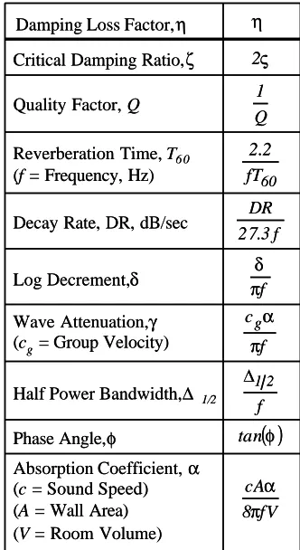
1.3.2 DAMPING LOSS FACTOR

The definition of damping in a SEA sense in given in equation 1.12. In other words, by considering the steady state power balance for a single isolated subsystem, it can be seen

that, Π = ωηE = 2πfηE. The input power is equal to

the energy dissipated. Furthermore, 2πη, like

efficiency, is the ratio of the input power to the energy dissipated by cycle.

Damping is by no means unique to SEA and no attempt is made here to conduct an exhaustive review of the wealth of pertinent information. Generally, analytical expressions are unavailable for most

systems. Typically, one must rely on empirical data or must conduct measurements to obtain damping

parameters. Linear viscous damping or an equivalent is by far the most common representation. Numerous

( )

( )

π π

ω = = (1.20)

ς 2 Q 1 60 fT 2 . 2 f 3 . 27 DR f π δ f c_g π α f 2 1 ∆ ( )φ tan fV 8 cA π α

Critical Damping Ratio, ζ Quality Factor, Q Reverberation Time, T₆₀ (f= Frequency, Hz) Decay Rate, DR, dB/sec Log Decrement, δ Wave Attenuation, γ (c_g= Group Velocity) Half Power Bandwidth, ∆ _1/2 Phase Angle, φ

Absorption Coefficient, α (c= Sound Speed) (A= Wall Area) (V= Room Volume)

Damping Loss Factor, η η

ς 2 Q 1 60 fT 2 . 2 f 3 . 27 DR f π δ f c_g π α f 2 1 ∆ ( )φ tan fV 8 cA π α

Critical Damping Ratio, ζ Quality Factor, Q Reverberation Time, T₆₀ (f= Frequency, Hz) Decay Rate, DR, dB/sec Log Decrement, δ Wave Attenuation, γ (c_g= Group Velocity) Half Power Bandwidth, ∆ _1/2 Phase Angle, φ

Absorption Coefficient, α (c= Sound Speed) (A= Wall Area) (V= Room Volume)

viscous damping descriptors exist and most are simply related as shown in Table 1.2. Two of the most common techniques for measuring damping are decay rate testing and the half power method. Decay rate methods involve acquiring a damping value from the

transient free decay of a response measurement. Typically, for frequency average SEA, this requires either pulse or filtered (in the band of interest) noise burst inputs. The response is also filtered in the same bandwidth of interest. The envelope of the free decay is then obtained by time averaging or Hilbert transform. The decay of the envelope can then be simply related to the damping loss factor either manually or by a least squares fit. The drawback is that the subsystem of interest must be isolated from the rest of the dynamic system. Breaking down a complex system under consideration into components or otherwise blocking the other components via mass loading or applied damping is often impractical or unrealistic. Alternatively, an in situ measurement of the damping loss factor may contain some error since not all of the measured loss is dissipative, some of the loss is simply energy transferred to other parts of the system. Furthermore, the method assumes that there truly exists an equipartition of energy and a constant damping value over the measured bandwidth. Use of the decay rate method alone does not allow for a quantified assessment of the degree to which these assumptions are or are not being met.

method is applied to a single resonance at a time (behaving as a single degree of freedom system in the vicinity of the natural frequency), the technique fails in frequency ranges where significant modal overlap occurs.

The SEA power balance for a single isolated subsystem can be used to infer damping.

Solving for the loss factor reveals that η = Π/(ωE). Thus, by measuring filtered (centered at

ω) steady state input power and response energy, the loss factor can be computed. Again,

however, this requires that the subsystem be practically or virtually isolated.

1.3.3 COUPLING LOSS FACTOR

The coupling loss factor is unique to SEA. Although defined in manner similar to the damping loss factor, the coupling loss factor represents power being transferred from one subsystem to another. The damping loss factor represents power dissipated by a subsystem. Physically, a damping mechanism may actually be a loss to some other medium. However, if the response of the other medium is of no interest, then it is not modeled as a SEA

subsystem. The associated coupling loss, therefore, is not represented but it is, instead, incorporated into the damping loss factor.

Coupling loss factors of idealized connections such as point, line, and area junctions can be determined using a mode or wave approach; see, for example, Cremer and Heckl [27], Lyon and Dejong [28], or Fahy [34]. Theoretical values for coupling loss factors are usually derived using the wave approach for semi-infinite systems, which is often simpler.

junctions exists in the literature. This can be readily applied to evaluate coupling loss factors. It is worth noting that SEA coupling parameters can be equivalently formulated using a mobility approach as discussed by Manning [37].

One of the earliest experimental approaches to verifying or identifying coupling loss factors is a method that uses the SEA power balance to solve for the coupling loss factor in terms of the measured subsystem energies and damping losses with respect to a single isolated

junction. The approach for two subsystems and a single junction is shown in Figure 1.13. By applying damping to subsystem 2, energy dissipated by subsystem 1 is negligible. Note, also, that only subsystem 1 is excited.

The power balance for subsystem 1 is:

Since the only appreciable energy dissipation occurs at subsystem 2, the input power, Π1 is

equal to the power dissipated in subsystem 2, ωη2E2. Hence, the power balance becomes:

Figure 1.13 Measurement of Coupling Loss

E1

Π1 Π2 = 0

ωη2E2

ωη1E1 = 0 ωη12E1

ωη21E2 E2

Damped

1 2 21 1

12E ωη E Π

Using the reciprocity relation, n1(ω)η12 = n2(ω)η21, and solving for the loss factor yields:

Again, the disadvantage here is that isolation of a single junction is required. This is likely to pose a great challenge if it is to be applied to a structure with any reasonable degree of complexity.

1.3.4 SUMMARY

In summary, the essence of SEA modeling is to evaluate the three main parameters: modal density, damping, and coupling. It is believed that subsystem modal density can be

accurately obtained for idealized systems since there is a firm theoretical basis and evidence of positive experimental results as shown by Hart and Shah [35], Clarkson [36], Clarkson and Pope [38], Szechenyi [39], and Keswick and Norton [40]. There is also reason to believe that the computation of theoretical coupling loss factors for idealized systems also maintains a fair degree of accuracy. On the other hand, an experimental approach must usually be taken to obtain damping loss factors for even the simplest systems. Furthermore, for any

reasonably complex structure, there is no firm procedure as to how to properly formulate any of the SEA parameters. This and the impracticality of component and/or junction isolation for complex structures suggest that there is a need for improved methods for experimentally

2 2 2 21 1

12E ωη E ωη E

ωη − = (1.22)

( )

( )

2 2 12

E n n E

E

ω ω η η

− =

1.4 EXPERIMENTAL SEA

A considerably limited amount of research effort has been conducted on experimental SEA. To date, some compelling work has been done mainly on somewhat simple structures; see, for example, Clarkson and Pope [38], Norton and Greenhalgh [41], and Wu et al [42]. However, it seems that further effort is required to examine the possibility and means of establishing a structured approach to the experimental identification of SEA parameters.

As was described previously, the direct measurement of SEA damping and coupling loss factors via subsystem and junction isolation methods is problematic. To overcome this, it seems obvious to attempt a more structured approach by simultaneously identifying all the elements of a coupling matrix from in situ response measurements. In fact, the idea of using the steady state power balance in an inverse manner was considered even early in SEA history. In Lyon and Dejong’s text [28], the idea is briefly discussed. Recall that since the coupling matrix, [β] (equation 1.19) for instance, is positive definite and usually diagonally

dominant, the process of inverting the matrix is numerically stable.

However, the inversion of a measured response matrix in the form of {[β]-1}-1 used to reconstruct (or identify) [β] may be numerically unstable. In fact, {[β]-1}-1 is extremely ill-conditioned for dynamic systems with moderate to high coupling. Specifically, this occurs

whenever the magnitude of the off-diagonal elements of [β] approach that of the diagonal

1.4.1 CLASSICAL POWER INJECTION METHOD

The earliest advance, by Bies and Hamid [43], to use the SEA power balance in an inverse manner is the development of the Power Injection Method (PIM). Basically, an experimental identification of loss factors for m subsystems is formed by inverting an m2xm2 matrix of measured steady state response energies. To illustrate, the three subsystem SEA model, shown in Figure 1.10, is used. First, the power balance is written for the case in which subsystem 1 is singly excited:

where, Ei(j) is the response energy of subsystem i due to excitation at subsystem j. For this

size system, the coupling matrix is given by:

Similarly, a power balance can be written for the other two cases where each of the remaining subsystems is singly excited:

The m individual power balance equations are combined into a single m2 x m2 matrix equation: (1.24)

[ ]

[ ]

(

)

(

)

(

)

[ ]

ω H

[ ]

Finally, equation 1.27 is solved to obtain the vector of loss factors by inverting the matrix of measured energies and then post multiplying by the vector of input powers.

Several drawbacks inherent to classical PIM are obvious. The dimension of the energy matrix increases with the square of the number of subsystems resulting in a substantial rise in computation time with increasing system complexity. Furthermore, the energy matrix has a tendency to be ill-conditioned due to the presence of significantly large off-diagonal terms. In fact, in this formulation, drive point energies, which tend to be the largest, are not

restricted to the diagonal.

1.4.2 IMPROVED POWER INJECTION METHOD

In attempt to overcome the computational difficulty associated with inverting a large energy matrix, Lalor [44] showed that by recombining the components of matrix equation 1.27, the damping loss factors could be separated from the coupling loss factors. The result is a simpler set of equations. Instead of m2 equations, the system is reduced to m sets of (m-1) x

(m-1) matrix equations for the coupling loss factors and a single m x m equation for the

damping loss factors. To illustrate for three subsystems, equation 1.27 is recombined to give:

which can be solved to yield the coupling loss factors. Also:

which can be solved to obtain the damping loss factors. Mathematically, the extension to higher order systems is straightforward.

Even though the problem is recast, exhibiting improved computational speed and diagonal dominance, Lalor shows that errors such as negative coupling can result. Additionally, the situation of moderate to high coupling still remains problematic in this improved PIM. Despite this, favorable results were obtained by Ming et al [45] using the method on an automobile rear section, though; the system was comprised of only eight subsystems.

1.4.3 NORMALIZED ENERGY INVERSION METHOD

As suggested by De Langhe [3], the most uncomplicated way to combine the individual power balance equations, 1.24 and 1.26, into a single matrix equation is via augmentation as follows:

As a matter of convenience, both sides of the equation can be normalized by the input powers to yield an equivalent form:

Denoting the normalized energies as Êi(j), where Êi(j) = ωEi(j)/Πi, yields:

[ ]

ω H (1.32)

For simplicity this can be written symbolically as:

Finally, the experimentally identified coupling matrix is, then, the inverted normalized energy matrix, [Ê]-1 obtained by solving equation 1.35. Obviously, this can readily be extended to systems of higher dimension.

Insight into the guidelines for acquiring a measured energy matrix exists in the literature. Hodges, et al [46] discuss some of the analytical properties possessed by the ideal [Ê] matrix revealed by examining its ideal equivalent, the [H]-1 matrix. The following observations can be made:

1) The inverse of [H] is non-negative everywhere. Indeed, this makes sense since all energy components are positive.

2) The inverse of [H] is weakly diagonally dominant. This also makes sense since the driven subsystem will always have the highest response.

3) If a measured [Ê] matrix is strictly positive and sufficiently diagonally dominant (light coupling), its inverse will yield a matrix with positive diagonal elements and negative off-diagonal elements. Note that this is the ideal form of [H].

4) If the inverse of a measured [Ê] matrix yields a matrix with positive diagonal & negative off diagonal elements and [A] is a diagonal matrix with all positive elements, then the inverse of [Ê]+[A] yields, yet, another matrix with positive diagonal & negative off diagonal elements. In other words, increasing the diagonal dominance of the measured energy matrix does not result in a non-ideal form for its inverse.

5) If the inverse of a measured [Ê] matrix yields a matrix with positive diagonal & negative off diagonal elements and [A] is a positive constant matrix, then the inverse of [Ê]+[A] yields a matrix with positive diagonal & negative off diagonal elements. This implies that, changing the relative variation of the off-diagonal elements of the measured energy matrix does not result in a non-ideal form for its inverse.

6) If any of the elements of a measured [Ê] matrix are zero, it is possible to reorder the matrix into a block-diagonal form with no zero elements in the blocks. This indicates that the only way to have subsystems with zero energy is if they are decoupled from the rest of the global system.

Using simulated systems, the authors, specifically, observe numerical difficulty whenever the energy of different subsystems was relatively close. This causes the energy matrix to be nearly singular with narrow quadratic form (evident in the large ratio between the largest and smallest eigenvalues; see figure 1.11) resulting in an identified coupling matrix with

1.5 CONCLUSIONS

To date, the normalized energy inversion method is apparently the best option for steady state SEA parameters identification. De Langhe [3] compares simulations of the normalized energy inversion method to the classical power injection method for identical systems of increasing dimension. The normalized energy method exhibits superior numerical conditioning and consumes less computational time, especially as system dimension

2 DEVELOPMENT OF A POWER FLOW MODEL REALIZATION

METHOD

2.1 PROBLEM DEFINITION AND APPROACH

Techniques to identify parameters from tests on low frequency second-order structural dynamic systems have been widely explored by the modal analysis community for over fifty years [49]. Advances were achieved in testing methods as well as system identification techniques. Early experimental efforts relied almost solely on analog testing. Two early modal identification contributions worth mentioning are “circle-fitting”, introduced by Kennedy and Pancu [50], and a systematic approach to normal mode testing developed by Lewis and Wrisley [51]. Prior to 1970, these two techniques (or variations of them) were used in most modal identification applications. After the introduction of computers into the laboratory and the development of the fast Fourier transform in the 1970’s, frequency response function testing and curve fitting gained popularity. Computational improvements beginning in 1980 resulted in the practical ability to conduct multiple input testing and led to enhancements in excitation, signal processing, and data analysis. Multiple input testing allowed multiple input system identification methods to be employed that offered improved results with increased speed; see, for example, Vold et al [52], Leuridan [53], Craig and Blair [54], and Zhang et al [55]. Also, a renewed interest developed in Auto-Regressive Moving Average (ARMA) techniques that were previously considered too computationally

modal parameters or to quantify structural changes to a system by tracking parameter

discrepancies in an accurate FEA model that has been updated using measured data from the modified structure.

System identification methods have also been widely explored by the automatic control community. This is due, at least, in part to the fact that an accurate system model is often required to develop an effective control scheme. Significant accomplishments in system identification in both the time and frequency domain have been made over the last thirty years. No attempt is made here to detail these developments. However, a technique in the field of controls that is related to modal identification is the process of constructing a space representation from measured data. This is usually termed system realization. Minimum order techniques developed by Ho and Kalman [57], which realize a model with the smallest state space dimension, have been successfully used to identify second order structural

dynamic systems [58]. In fact, as Juang [59] points out, minimum realization of a state space model in the time domain is computationally similar to the multiple input/multiple output time-domain methods often used by the modal testing community.

It seems that the question of how to identify SEA parameters from measured data is conceptually similar to the question of how to identify structural dynamic FEA parameters from measured data. Historically, the advancement of modal testing was not significantly motivated by seeking to improve FEA models. Not only do properly identified modal

some insight into the practicality of the power injection and energy inversion methods for use in SEA can be obtained by considering the similar problem of obtaining FEA parameters from an inversion of measured response data. The first obvious conclusion is that it is, indeed, quite impractical to attempt to measure input/output data on a structure at all

locations where there are finite element nodes in its model. Similarly, it is likely that not all SEA degrees of freedom will be measured, especially, in plane extension or shear modes. Second, inversion of this response matrix from modal tests would suffer from poor numerical conditioning for reasons similar to that for a measured energy response matrix. Nonetheless, there exist FEA updating methods that have proven successful. This is done not by directly measuring physical parameters but by focusing instead on modal parameters, which serve as the common ground between structural dynamic modeling and test.