NON-SEPARABLE REGULARIZATION BASED DE- CONVOLUTION

1244 | P a g e

NON-SEPARABLE REGULARIZATION BASED

DE-CONVOLUTION

K. Rajitha, M.Tech

1

, J. Sheshagiri Babu, M.Tech.(Ph.D)

2

1,2

ECE, Kakatiya Instistute of Technology and Science, Warangal, (India).

ABSTRACT

A standard convex approach for sparse one-dimensional de-convolution improves upon L1-norm regularization.

We propose a sparsity -inducing non-separable non-convex bivariate penalty function for this purpose. It is

designed to enable the convex formulation of ill- conditioned linear inverse problems with quadratic data

fidelity terms. The new penalty overcomes limitations of separable regularization. We show how the penalty

parameters should be set to ensure that the objective function is convex, and provide an explicit condition to

verify the optimality of a prospective solution. In this project, We present an algorithm (an instance of

forward-backward splitting) for sparse de-convolution using the new penalty terms.

Key Words-

De-Convolution, Convex Functions, Sparse Signal Estimation, Non-Convex Regularization.

I.

INTRODUCTION

In this literature we are going to deal with sparse regularization. This sparse regularization can be categorized

into two types. One is convex and other one is non-convex. In this project we are using the term regularization

terms is called as penalty functions. In the convex approach, the regularization terms or penalty functions are

convex. The convex method consisting of both data fidelity and regularization terms. So that the objective

function is convex [1], [2]. By using this convex approach method we have several advantages i.e., the

objective function is free of extraneous (irrelevant) local minima, and globally convergent optimization

algorithms can be improved [3].

The Non-convex regularization has more advantages [4], [5], [6] comparative to convex regularization .

Classical and recent examples of non-convex method is edge preserving tomography [7], [8], [9], [10] and

compressed sensing [11], [12], [13], respectively. By using these techniques the non-convex approach performs

better than convex one’s. In the convex approach, penalty functions are convex. Because these non-convex functions are designed to induce sparsity more effectively than non-convex one’s. therefore the non-convexity of

the objective function is generally sacrificed. Non-convex regularization is having some complications that is

the objective function will generally posses many sub-optimal local minima in which optimization algorithms

can become entrapped.

It turns out, without giving up the convexity of the objective function and corresponding benefits. The

non-convex penalties can be utilized. This is achieved by carefully specifying the penalty in accordance with the data

1245 | P a g e

sparcity-inducing non-convex penalties has been developed to formulate convex objective functions and applied

to several signal estimation problems [16], [17], [18], [19], [20], [21], [22], [23], [24]. This approach maintains

the benefits of the convex framework (absence of spurious local minima, etc.), yet estimates sparse signals more

accurately than convex regularization (e.g., the

l

₁norm) due to the sparsity –inducing properties of non-convex

regularization. However , this previous work considers only separable (additive) penalties, which have

fundamental limitations.

In this paper, we introduce a parameterized sparsity-inducing non separable non-convex bivariate penalty

function. To enable the convex formulation of ill-conditioned linear inverse problems with quadratic data

fidelity terms the penalty function is designed. The new penalty overcomes the limitations of separable

non-convex regularization. In this paper, now we show how the penalty parameters should be set to ensure the

objective function is convex. And we also show how this bivariate penalty can be incorporated into linear

inverse problems of

N

variables

(

N



2)

, and then we provide an explicit condition to verify the optimality

of a prospective solution. For sparse signal reconstruction using the new penalty we present an iterative

algorithm (as instance of forward-backward splitting), and we demonstrate it’s effectiveness for

one-dimensional sparse de-convolution.

A. Notation

We write the vector

x



R

Nas

x





x x

₁

,

_2,....,

x

_N



. Given

x



R

N, we define

x

_n



0

for

n



{1, 2,...., }

N

. (This simplifies expressions involving summations over

n

.) The

l

₁norm of

x



R

Nis defined as

1

|

n

|

n

x





x

 

. If the matrix

A

is positive semi definite, we write

A



0

. If the

A B



is positive semi

definite, we write

A



B

.

II.

SPARSE RECONSTRUCTION

In signal processing the practical problems are involve far more than two variables. Therefore, the proposed

bivariate penalty and convexity condition are of little practical use on their own. In this section we show how

they can be used to solve an

N

- point linear inverse problem (with

N



2

). We consider the problem of estimating a signal

x



R

N given

y

,

y



Hx



w

(1)

Where

H

is a known linear operator,

x

is known to be sparse, and

w

is additive white Gaussian noise

(AWGN). we formulate the estimation of

x

as an optimization problem with bivariate sparse regularization

1246 | P a g e

 

2









2 1

1

arg min{

,

;

}

2

2

N n n

x R _n

x



F x

y

Hx





x

_

x

a

















(2)

Where





0

,

a





a a

₁

,

₂



and



:

R

2



R

is the proposed bivariate penalty. In the penalty term, the first

and last signal value pairs,



x x

₀

,

₁



and



x

_N

,

x

_N1



, straddle the end-points of

x

.

C

, we define

x

n



0

for

{1, 2,..., }

n



N

, which simplifies subsequent notation.

If

a

₁



a

₂, then the bivaiate penalty is separable, i.e.,



  

u a

;





u a

₁

;

₁

 





u a

₂

;

₁



, and the

N

-point

penalty term in (2) reduces to



_n

;

₁



n

x a

 



. Hence, we recover the standard (separable) formulation of

sparse regularization. In particular, if

a

₁



a

₂



0

, then



 

u

;0



|

u

₁

|



|

u

₂

|

and the

N

-point penalty term

reduces to



 

x

₁, i.e., the classical sparsity-inducing convex penalty.

In order to induce sparsity more effectively, we allow



to be non-separable; i.e.,

a

₁



a

₂. To that

end, the following section addresses the problem of how to set

a

₁ and

a

₂ in the bivariate penalty



to ensure

convexity of the

N

- variate objective function

F

in (2).

The lemma is proven in appendix D. According to the lemma, it is sufficient to restrict



so as to ensure

convexity of the bivariate function

f

in (3). Therefore , the allowed penalty parameters

a

_i can be determined from the tridiagonal matrix P. using lemma 1, we obtain theorem 1.

A.

Optimality Condition

In this section, we derive an explicit condition to verify the optimality of a prospective minimize of the objective

function

F

in (2). The optimality condition is also useful for monitoring the convergence of an optimization

algorithm (see the animation in the supplemental material).

The general condition to characterize minimiers of a convex function is expressed in terms of the sub

differential. If

F

is convex, then

x

opt



R

N is a minimizer if and only if

0



F x

 

opt where



F

is the sub differential of

F

.

We seek an expression for the sub differential of the objective function

F

. The function

F

in (2) has a

regularization term that is non-differentiable, non-convex, and non-separable. But using , we may write the

1247 | P a g e







1



1

,

;

2

n n n

x

x

a



_



(3)







1





1



1

1

[

,

;

,

]

2

n n n n n

S

x

_

x

a

x

_

x











(4)

= ₁

1





₁

,



;



2

n n n

x





S

x

_

x

a

 

(5)

Where

x

_n



0

for

n



{1, 2,..., }

N

. We define

:

N

R

R





as

 





1





1

,

,

;

2

n n n

x a

S

x

_

x

a







(6)

The function



is twice continuously differentiable because it is the sum of twice differentiable functions.

Using (5), we ,may express the objective function

F

in (2) as

 

1

₂2

 

;

₁

2

F x





y



Hx



 



x a





 

x

(7)

The benefit of (7) compared to (2) is that the regularization term ( which is non-differentiable, non-convex, and

non- separable ) is separated into a differentiable part and a convex separable part. The



term is differentiable

and its gradient is easily evaluated. The

l

₁norm is separable and convex and its sub differential is easily

evaluated.

The gradient of



is given by

 

;

1

₁





,

₁



;



1

₂





₁

,



;



2

n n

2

n n

n

x a

S

x x

_

a

S

x

_

x

a















(8)

Where

S

_i is the partial derivative of

S





x x

₁

,

₂





with respect to

x

_i. The sub differential of the

l

₁ norm is separable [11],

1248 | P a g e

 



 



 

1 ,

0

: { 1,1 ,

0

1 ,

0

t

sign t

t

t

 









(10)

Since the first two terms of (7) are differentiable, the sub differential of

F

is



F x

 



H

T



Hx



y



 



 

x a

;

 



 

x

₁. (11)

Hence the condition

0

 

opt

F x



can be expressed as



1/





H

T



y



Hx

opt







x

opt

;

a







x

opt



₁ (12)

Expressing this condition component-wise, we have the following result.

B.

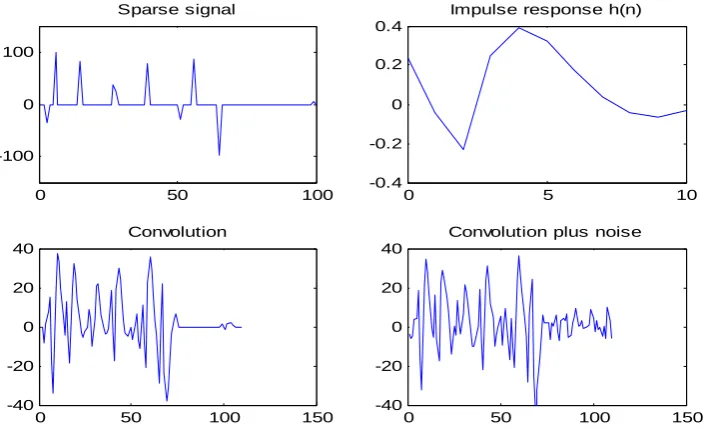
Sparse Deconvolution

We apply theorem 1 to the sparse deconvolution problem. In this case, the linear operator

H

represents

convolution, i.e.,

 

n n k k

k

Hx





h

_

x

(13)

That is,

H

is a Toeplitz matrix. It represents a linear time-invariant (LTI) system with frequency response

given by the Fourier transform of

h

,

 

jwn

n n

H w





h e

 (14)

Similarly, the matrix

P

in (2a) represents an LTL system with a real-valued frequency response,

 

1 0 1

jw jw

P w



p e





p



p e

(15)

0

2

1

cos( )

p

p

w





(16)

1249 | P a g e

III.

FIGURES

0 0.5 1 1.5 2 2.5 3

0 0.2 0.4 0.6 0.8 1

Frequency ()

|H()|2 P()

Fig.1. Filters

H w

 

and

P w

 

for example 2.

0 50 100

-100 0 100

Sparse signal

0 5 10

-0.4 -0.2 0 0.2 0.4

Impulse response h(n)

0 50 100 150

-40 -20 0 20 40

Convolution

0 50 100 150

-40 -20 0 20 40

Convolution plus noise

1250 | P a g e

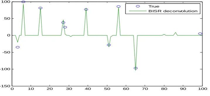
0 10 20 30 40 50 60 70 80 90 100

-150 -100 -50 0 50 100

True

BISR deconvolution

Fig .3. example 2 of sparse deconvolution using BISR.

IV.

COMPARISION TABLE

Algorithm RMSE No of iterations

1

l

norm De-convolution 4.70 32

Proposed De-convolution 3.11 22

V.

CONCLUSION

The results and comparison table show that Proposed De-convolution gives RMSE value better than

l

₁ norm

De-convolution. The signal can be exactly or more approximated estimated using the proposed de-De-convolution.

REFERENCES

[1] F. Bach, R. Jenatton, J. Mairal, and G. Obozinski, “optimization with sparsity-indusing penalties,” Found.

Trends Mach. Learn., vol. 4, no. 1,pp. 1-106, 2012.

[2] Convex optimization in signal processing and communications, D. P. Palomar and Y. C. Eldar, Eds.

Cambridge, U.K.: Cambridge Univ. press, 2010.

[3] S. Boyd and L. Vandenberghe, Convex Optimization. Cambridge, U.K.: Cambridge Univ. Press, 2004.

[4] A.Bruckstein, D. Donoho, and M. Elad, “From sparse solutions of systems of equations to sparse modeling

of signals and images,” SIAM Rev., vol. 51, no. 1, pp. 34–81, 2009.

[5] A.Bruckstein, D. Donoho, and M. Elad, “From sparse solutions of systems of equations to sparse modeling

of signals and images,” SIAM Rev., vol. 51, no. 1, pp. 34–81, 2009.

[6] M. Nikolova, “Energy minimization methods,” in Handbook of Mathematical Methods in Imaging, O.

1251 | P a g e

[7] P. Charbonnier, L. Blanc-Feraud, G. Aubert, and M. Barlaud, “Deterministic edge-preserving regularization

in computed imaging,” IEEE Trans. Image Process., vol. 6, no. 2, pp. 298–311, Feb. 1997.

[8] D. Geman and G. Reynolds, “Constrained restoration and the recovery of discontinuities,” IEEE Trans.

Pattern Anal.Mach. Intel., vol. 14, no. 3, pp. 367–383, Mar. 1992.

[9] M. Nikolova, “Markovian reconstruction using a GNC approach,” IEEE Trans. Image Process., vol. 8, no.

9, pp. 1204–1220, 1999.

[10]M. Nikolova, M. K. Ng, and C.-P. Tam, “Fast nonconvex nonsmooth minimization methods for image

restoration and reconstruction,” IEEE Trans. Image Process., vol. 19, no. 12, pp. 3073–3088, Dec. 2010.

[11]R. Chartrand, “Fast algorithms for nonconvex compressive sensing: MRI reconstruction from very few

data,” in Proc. IEEE Int. Symp. Biomed. Imag. (ISBI), Jul. 2009, pp. 262–265.

[12]R. Chartland, E. Y. Sidky, and P. Xiaochuan,” Non convex compressive sensing for X-ray CT: An

algorithm comparision,” in proc. Asilomar conf, Signals, syst., comput., Nov. 2013, pp. 665-669.

[13]J. Trzasko and A. Manduca, “Highly under sampled magnetic resonance image reconstruction via homo

topic L0-minimization,” IEEE Trans. Med. Imag., vol. 28, no. 1, pp. 106-121, Jan. 2009.

[14]A. Blake and A. Zisserman, Visual Reconstruction. Cambridge, MA, USA: MIT Press, 1987.

[15]M. Nikolova, “Estimation of binary images by minimizing convex criteria,” in Proc. IEEE Int. Conf. Image

Process. (ICIP), 1998, vol. 2, pp. 108–112.

[16]I. Bayram, “penalty functions derived from monotone mappings,” IEEE Signal process. Lett., vol. 22,

no. 3, pp. 265-269, Mar.2015.

[17]I. Bayram, P.-Y. Chen, and I. Selesnick, “Fused lasso with a nonconvex sparsity inducing penalty,” in Proc.

IEEE Int. Conf. Acoust., Speech, Signal Process. (ICASSP), Florence, Italy, May 2014.

[18]P. Y. Chen and I. W. Selesnick, “Group-sparse signal denoising: Non-convex regularization, convex

optimization,” IEEE Trans. Signal Process., vol. 62, no. 13, pp. 3464–3478, Jul. 2014.

[19]Y. Ding and I. W. Selesnick, “ Artifact-free wavelet denoising: Non-convex sparse regularization, convex

optimization,” IEEE signal process. Lett., vol. 22, no. 9, pp. 1364-1368, Sept. 2015.

[20]A. Lanza, S. Morigi, and F. Sgallari, “Convex image denoising via non-convex regularization,” in Scale

Space and VariationalMethods in Computer Vision, ser. Lecture Notes in Computer Science, J.-F. Aujol,

M. Nikolova, and N. Papadakis, Eds. New York, NY, USA: Springer, 2015, vol. 9087 , pp. 666–677.

[21]A. Parekh and I. W . Selesnick, “Convex denoising using non-convex tight frame regularization,” IEEE

Signal Process. Lett., vol. 22, no. 10, pp. 1786-1790, Oct. 2015.

[22]A. Parekh and I. W . Selesnick, “Convex fused Lasso denoising with non-convex regularization and its use

for pulse detection,” Oct. 2015 [online] . Available: http://arxiv.org/abs/1509.02811.

[23]I. W. Selesnick and I. Bayram, “Sparse signal estimation by maximally sparse convex optimization,” IEEE

Trans. Signal Process., vol. 62, no. 5, pp. 1078–1092, Mar. 2014.