Quantitative Techniques for Spread Trading in Commodity Markets

(1)

Western University Western University

Scholarship@Western

Electronic Thesis and Dissertation Repository

5-11-2015 12:00 AM

Quantitative Techniques for Spread Trading in Commodity

Markets

Mir Hashem Moosavi Avonleghi The University of Western Ontario

Supervisor Dr. Matt Davison

The University of Western Ontario

Graduate Program in Statistics and Actuarial Sciences

A thesis submitted in partial fulfillment of the requirements for the degree in Doctor of Philosophy

Follow this and additional works at: https://ir.lib.uwo.ca/etd

Part of the Statistical Models Commons

Recommended Citation Recommended Citation

Moosavi Avonleghi, Mir Hashem, "Quantitative Techniques for Spread Trading in Commodity Markets" (2015). Electronic Thesis and Dissertation Repository. 2849.

https://ir.lib.uwo.ca/etd/2849

This Dissertation/Thesis is brought to you for free and open access by Scholarship@Western. It has been accepted for inclusion in Electronic Thesis and Dissertation Repository by an authorized administrator of

(2)

QUANTITATIVE TECHNIQUES FOR SPREAD TRADING

IN COMMODITY MARKETS

(Thesis format: Monograph)

by

Mir Hashem Moosavi Avonleghi

Graduate Program in Statistics and Actuarial Science

A thesis submitted in partial fulfillment

of the requirements for the degree of

Doctor of Philosophy

The School of Graduate and Postdoctoral Studies

The University of Western Ontario

(3)

Abstract

This thesis investigates quantitative techniques for trading strategies on two com-modities, the difference of whose prices exhibits a long-term historical relationship known as mean-reversion. A portfolio of two commodity prices with very similar characteristics, the spread may be regarded as a distinct process from the underlying price processes so deserves to be modeled directly. To pave the way for modeling the spread processes, the fundamental concepts, notions, properties of commodity markets such as the forward prices, the futures prices, and convenience yields are described. Some popular commodity pricing models including both one and two factor models are reviewed. A new mean-reverting process to model the commodity spot prices is introduced. Some analytical results for this process are derived and its properties are analyzed. We compare the new one-factor model with a common existing one-factor model by applying these two models to price West Texas Intermediate (WTI) crude oil, and discuss its advantages and disadvantages. We investigate the recent behavioral change in the location spread process between WTI crude oil and Brent oil.

The existing three major approaches to price a spread process namely cointegra-tion, one-factor and two-factor models fail to fully capture these behavioral changes. We, therefore, extend the one-factor and two-factor spread models by including a compound Poisson process where jump sizes follow a double exponential distribution. We general-ize the existing one-factor mean-reverting dynamics (Vasicek process) by replacing the constant diffusion term with a nonlinear term to price the spread process. Applying the new process to the empirical location spread between WTI and Brent crude oils dataset, it is shown how the generalized dynamics can rigorously capture the most important characteristics of the spread process namely high volatility, skewness and kurtosis. To consider the recent structural breaks in the location spread between WTI and Brent, we incorporate regime switching dynamics in the generalized model and Vasicek process by including two regimes.

We also introduce a new mean-reverting random walk, derive its continuous time stochastic differential equation and obtain some analytical results about its solution. This new mean-reverting process is compared with the Vasicek process and its advantages dis-cussed. We showed that this new model for spread dynamics is capable of capturing the possible skewness, kurtosis, and heavy tails in the transition density of the price spread process. Since the analytical transition density is unknown for this nonlinear stochastic process, the local linearization method is deployed to estimate the model parameters. We apply this method to empirical data for modeling the spread between WTI crude oil and West Texas Sour (WTS) crude oil.

Finally, we apply the introduced trading strategies to empirical data for the location spread between WTI and Brent crude oils, analyze, and compare the profitability of the strategies. The optimal trading strategies for the spread dynamics in the cointegration approach and the one-factor mean-reverting process are discussed and applied to our considered empirical dataset. We suggest to use the stationary distribution to find

(4)

mal thresholds for log-term investment strategies when the spread dynamics is assumed to follow a Vasicek process. To incorporate essential features of a spread process such as skewness and kurtosis into the spread trading strategies, we extend the optimal trading strategies by considering optimal asymmetric thresholds.

Keywords: Pairs trading; Commodity pricing model; Commodity spread process;

Con-venience Yield; Cointegration; Mean-reversion; Energy markets; Mean-reverting ran-dom walk; The Kalman filter; Optimal Trading Strategy; Regime Switching Algorithm; Ornstein-Uhlenbeck process; Crude Oil Futures Prices

(5)

Acknowledgements

First of all, I would like to express my sincere gratitude to my supervisor, Professor Matt Davison, for his invaluable guidance and continued support, and immense knowl-edge. This thesis would not have been possible without his substantiable help and his long-lasting patience. I am appreciative of his generosity with his time and for great stimulating discussions.

I wish to extend my warmest thanks for the advice that I received from Dr. Adam Metzler during the time I studied for my Master’s degree at Applied Mathematics Department and his leading me to make the right choice. I would like to express grateful thanks to Dr. Mark Reesor for his guidance and leading financial modeling group. I am grateful to all of the people who helped in the various stages of this research. I would also like to express my sincere thanks to the members of my thesis examiners.

I acknowledge the Department of Statistical and Actuarial Sciences and the Faculty of Graduate Studies for their financial support. I would also like to thank to Jennifer Dungavell (Administrative Officer), Jane Bai (Academic Coordinator), and Keri Knox (Professional Education Coordinator) for their assistance.

Special thanks also go to my friends Ali Akbar Mohsenipour, Azaz Bin Sharif, and Mehdi Taheri for their support and encouragement.

Finally, I express my thanks to all my other friends and colleagues who provided great company for all these years I spent at Western. Thank you for making academic life tolerable and for the excellent memories that I will never forget.

(6)

Dedicated To:

My Parents My Sisters

And My Brothers

Thank you for your love, support and encouragement

(7)

List of Figures

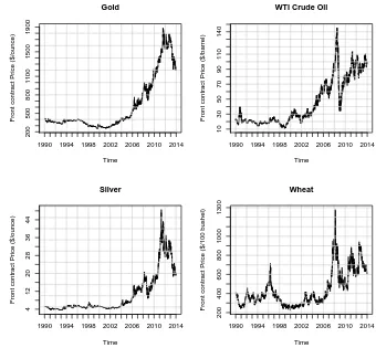
1.1 The front contracts daily futures prices for Gold, Silver, Wheat, and WTI crude oil from 1990-01-02 to 2013-12-31. . . 6

2.1 Time plot of the simulated data and fitting model to the ARM A(2,1) model in equation 2.47: Plot (a) shows the 1000 simulated series and its corresponding filtered series. Plot (b) checks for linear serial correlation in the residual series through ’acf’. Here, we use 5610 as a seed to generate this series. . . 30

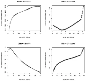
3.1 The observed futures prices for WTI crude oil in given dates and their corresponding fitted forward curves using smoothing B-spline. . . 36

3.2 Implied convenience yields derived using the futures contracts of 2 and 3 months to maturities for the daily futures prices of WTI crude oil staring from January 2, 2001 to September 6, 2011. For simplicity, we considered the short interest rates rt constant and equal to 0.05. . . 38

3.3 The interpolated convenience yields using smoothing B-spline for WTI crude oil in given dates, which their corresponding fitted forward curves are plotted in figure3.1. For simplicity, in these graphs, we considered the short interest rates rt,s to be constant and equal to 5% for all dates and

maturities. . . 39

3.4 Time plot of the daily front futures prices for WTI crude oil from January 2, 2001 to September 6, 2011 using one-factor method: Plot (a) shows the estimated state variable (filtered spot price) and the front contract futures prices. Plot (b) shows the daily futures prediction errors corresponding to front and second futures contracts (the futures contracts of 1,2,3,4 and 5 month maturities are used in the estimation). . . 47

3.5 Time plot of the daily front futures prices for WTI crude oil from January 2, 2001 to September 6, 2011: Plot (a) shows the estimated filtered spot prices and the front contract futures prices derived by two-factor model. Plot (b) shows the estimated filtered convenience yield derived by two-factor model (the futures contracts of 1,2,3,4 and 5 month maturities are used in the estimation). . . 55

(11)

3.6 The plot depicts comparison between empirical transition densities for log-processes in the new model and Schwartz (1997)’s models after five years using 10,000 simulated paths. Here it is assumed κ = 3.2, µ =

−0.86, σ = 0.3, and θ = 6 for this new process 3.62 and we also assumed κ = 0.27, µ = 4.62, σ = 0.3 for the Schwartz (1997)’s process 3.19. For both models, ∆t = ₂₅₂1 , and T = 5 are assumed using identical random generated numbers. . . 58

3.7 Left plot show time plot of the daily front futures prices for WTI crude oil from October 1, 2004 to December 31, 2014 (price in $/barrel). Right plot depicts the empirical density of the logarithm of the same dataset, given in the left plot. . . 61

3.8 The plot shows comparison between the empirical density for the logarithm of observed daily WTI front futures prices staring from October 1, 2004 to December 31, 2014 with the fitted stationary distributions of these two models namely Schwartz one-factor and the new generalized one-factor for log-spot prices. The fitted parameters are summarized in table3.3. . . . 63

4.1 The time plots are simulated series for xt (solid line) and yt (dotted line)

based on model4.2when µ1 = 0.2, µ2 = 0.5, and variances of innovations

are 1. Number of simulations is 500 and 56984 is used as seed to generate the series. . . 69

4.2 The time plots are simulated series fory1,t andy2,t and their cointegration

residuals based on model (4.5) when variances of i.i.d white noises ε1,t

and ε2,t are 1. Number of simulations is 500 and 2987 is used as seed to

generate series. . . 70

4.3 The time plots are simulated series for y1,t and y2,t and their

autocorrela-tion funcautocorrela-tions based on model (4.10) when variances of i.i.d white noises ε1,t and ε2,t are 1. Number of simulations is 500 and 6987 is used as seed

to generate series. . . 73

4.4 The monthly front contracts future prices for WTI crude oil and Brent oil from April 1994 to January 2005 (price in $/barrel). . . 76

4.5 The monthly front contract location spread between WTI crude oil and brent oil from April 1994 to January 2005 (spread in $/barrel). . . 80

4.6 Elliot’s model parameters estimation showing how parameters evolve in optimization’s function generated by Kalman filter. As we can see, after some iterations, all parameters along with maximum likelihood function converge and stabilize. The data set is monthly location spread between WTI and Brent oils for future contracts of 1,3,6,9 and 12 months to ma-turities from April 1994 to January 2005. . . 81

4.7 Compare Elliot’s model filtered spot spread series with the front contract monthly realization. The data set that is used to estimate filter spot spread is monthly location spread between WTI and Brent oils for future contracts of 1,3,6,9 and 12 months to maturities from April 1994 to January 2005 . 82

(12)

4.8 Compare Dempster’s model filtered spot spread series with the front con-tract monthly realization. The data set that is used to estimate filter spot spread is monthly location spread between WTI and Brent oils for future contracts of 1,3,6,9 and 12 months to maturities from April 1994 to January 2005. . . 89

4.9 Dempster’s model parameters estimation showing how estimates of pa-rameters evolve in optimization’s function for Kalman filter. As we can see, after some iterations, all parameters along with maximum likelihood function converge and stabilize. The data set is monthly location spread between WTI and Brent oils for future contracts of 1,3,6,9 and 12 months to maturities from April 1994 to January 2005. . . 90

4.10 The daily front contract of WTI crude oil prices and Brent crude oil prices and their location spread series from April 1994 to November 2013 (price in $/barrel). . . 91

4.11 The empirical distributions using the three different parameter settings for the generalized on-factor mean-reverting process. We simulated 10,000 paths where the ∆t = ₂₅₂1 , and T = 5 are considered using identical random generated numbers. . . 96

4.12 The plot depicts the stationary solutions (distributions) for this mean-reverting process given in the SDE form in equation 4.59 in which its derived stationary solution is in equation 4.65. Here, we have set κ = 1, µ= 1, σ = 1, ν = 0.4 and θ = 2. . . 98

4.13 The left plot depicts comparison between the empirical density for the ob-served daily spread between WTI and Brent crude oils data (April 1994 to December 2010) in first regime with the fitted stationary distributions of these two models: Vasicek and generalized one-factor mean-reverting. The right plot shows the comparison between the empirical density for the observed daily spread between WTI and Brent crude oils data (January 2011 to November 2013) in second regime with the fitted stationary dis-tributions of these two models. The fitted parameters are summarized in table 4.7 in both regimes. . . 104

5.1 The daily front contract of WTI crude oil prices and spot WTS crude oil prices and their spread series from January 2000 to January 2013 (price in $/barrel). . . 108

5.2 The plot depicts the empirical density of the observed daily spread between WTI and WTS crude oil from January 2000 to January 2013. . . 109

5.3 Left panel is difference of standardized spread (spread_σ_(spread)−µ(spread)) vs stan-dardized spread, showing slight evidence of mean-reversion. To show the pattern more clearly, we binned the horizontal axis into 25 bins of equal width; calculate the average of the points in the bins in right panel. This shows mean-reversion more clearly. . . 110

(13)

5.4 Comparison between simulated probability density functions ofXt for the

SDE in equation 5.18 for given parameters. Here, for all these three ran-dom walks, we assumed κ = 1, σ = 1, ∆t = 1/252 , T = 1 and 100,000 simulated paths. . . 116

5.5 The plot depicts the stationary solutions (distributions) for the MRW given in the SDE form in equation 5.18 in which its derived stationary solution is in equation 5.25. By looking these graphs, we can see that as a increases, the stationary distribution has higher peak and thinner tails. Here, for these two stationary solutions, we assumed κ= 1, σ = 1. . . . 118

5.6 The plot depicts the drift functions for the new mean-reverting process given in equation5.41 and the Vasicek process given in equation 5.1. We assumedκ= 1, µ= 0 for both models. . . 122

5.7 Time plots of variance and empirical densities for 10,000 simulated paths: Plot (a) shows how empirical variances evolve through the time in these three models. Plot (b) shows comparison between empirical densities in these two models after five years. We assumed κ = 0.4, µ = 0, σ = 1, ∆t = ₂₅₂1 , and T = 5 for both models by using identical random generated numbers. . . 123

5.8 The plot depicts comparison between empirical densities in these two mod-els after five years using 10000 simulated paths. We assumed κ = 4, µ= 0.3, σ= 2.1 for this new process 5.41 and we also assumed κ= 0.86, µ = 1.2, σ = 2.1 for the Vasicek process 5.1. for both models ∆t = 1

252,

and T = 5 are considered by using identical random generated numbers. 124

5.9 The plot depicts the fitted drift functions for the new mean-reverting pro-cess and the Vasicek propro-cess using the time scaled estimated parameters for κ, and µthat are summarized in table 5.3. . . 128

5.10 The empirical distributions using the fitted parameters (summarized in table5.3) for both the Vasicek and the new mean-reverting processes with their time scaled dynamics. The left plot compares the results for the fitted with its time scaled for the new mean-reverting process and right plot compares for the results for the fitted with its time scaled for Vasicek process. We simulated 10,000 paths for four fitted processes with ∆t= ₂₅₂1 , andT = 15 are considered using identical random generated numbers with 21745 as a seed. . . 129

5.11 The left plot depicts comparison between simulated empirical densities in these two models: Vasicek and the new mean-reverting after fifteen years using 10,000 simulated paths using the fitted parameters (summarized in table 5.3). The right plot shows the comparison between the empirical density for the observed daily spread between WTI and WTS crude oil data with the fitted stationary distributions of these two models. We assumed that the ∆t = ₂₅₂1 , andT = 15 using identical random generated numbers with 21745 as a seed for the simulation. . . 130

(14)

6.1 Time plot of the estimated spread process between WTI crude oil and Brent oil daily front contracts prices from April 1994 to January 2005 in cointegration approach: Plot (a) shows the series of trades in strategy (a) in which whenever we hit the lower barrier, `1 = µ−∆ = 0−0.816 or

upper barrier,`2 =µ+ ∆ = 0 + 0.816, we close existing paired trade and

open new position in opposite direction. Plot (b) shows the series of trades in strategy (b) in which whenever we hit the lower barrier,`1 =µ−∆ =

0−0.816 or upper barrier, `2 = µ+ ∆ = 0 + 0.816, we only open a new

position in proper direction and we wait until to revert to long-run mean, 0 when we unwind existing paired trade. Plot (c) depict how profit/loss growth is both strategies. . . 135

6.2 Time plot of the location spread process between WTI crude oil and Brent oil daily front contracts prices from April 1994 to January 2005 in one-factor method: Plot (a) shows the series of trades in strategy (a) in which whenever we hit the lower barrier, `1 = b−∆ = 1.649−0.843 or upper

barrier, `2 = b + ∆ = 1.649 + 0.843, we close existing paired trade and

open new position in opposite direction. Plot (b) shows the series of trades in strategy (b) in which whenever we hit the lower barrier, `1 = b−∆ =

1.649−0.843 or upper barrier,`2 =b+ ∆ = 1.649 + 0.843, we only open

a new position in proper direction and we wait until to revert to long-run mean, b = 1.649 when we unwind existing paired trade. Plot (c) depict how profit/loss growth is both strategies. . . 139

6.3 The plot depicts the optimal amount of sigma away from long-run mean in the given profitability measure function for a Gaussian white noise . . 141

6.4 Time plot of the location spread process between WTI crude oil and Brent oil daily front contracts prices from April 1994 to January 2005 in one-factor method: Plot (a) shows the series of trades in revised strategy (a∗) in which whenever we hit the lower barrier,`1 =b+ ∆1 = 1.649−0.632 or

upper barrier,`2 =b+ ∆2 = 1.649 + 1.345, we close existing paired trade

and open new position in opposite direction. Plot (b) shows the series of trades in revised strategy (b∗) in which whenever we hit the lower barrier, `1 =b+ ∆1 = 1.649−0.628 or upper barrier,`2 =b+ ∆2 = 1.649 + 1.346,

we only open a new position in proper direction and we wait until to revert to the proper closing barriers: `3 =b+ ∆3 = 1.649 + 0.189 (when existing

trade was opened at `1) or `4 = b + ∆3 = 1.649 + 0.332 (when existing

trade was opened at `2) when we unwind existing paired trade. Plot (c)

depict how profit/loss growth is both strategies. . . 146

(15)

List of Tables

2.1 Estimated parameters for 1000 sample size data generated based on the ARM A(2,1) model in equation 2.47 using the Kalman filter algorithm. . 26

3.1 Estimated parameters for one-factor model using the futures contracts of 1,2,3,4 and 5 months to maturities (the daily prices of WTI crude oil stating from January 2, 2001 to September 6, 2011). . . 46

3.2 Estimated parameters for this two-factor model using the futures contracts of 1,2,3,4 and 5 months to maturities (the daily prices of WTI crude oil staring from January 2, 2001 to September 6, 2011). . . 54

3.3 Estimated parameters for these two processes namely the new generalized one-factor and Schwartz one-factor models based on the observed daily WTI front futures prices from October 1, 2004 to December 31, 2014. . . 62

4.1 Regression results based on model (4.2) when µ1 = 0.2, µ1 = 0.5, and

variances of innovations are 1. Number of simulations is 500 (y ∼x) and 56984 is used as seed to generate series. . . 68

4.2 Unit root tests for WTI and Brent front monthly contracts future price series and their differenced series from April 1994 to January 2005. . . . 77

4.3 The Johansen test results to check whether WTI crude oil and Brent oil prices for the specified data ( monthly front contract prices from April 1994 to January 2005) are cointegrated or not. . . 77

4.4 Estimated parameters for Elliott’s one factor model using monthly location spread between WTI and Brent oils for future contracts of 1,3,6,9 and 12 months to maturities from April 1994 to January 2005. . . 81

4.5 Estimated parameters for Dempster’s two factor model using monthly fu-ture location spread between WTI and Brent oils from April 1994 to Jan-uary 2005 and comparison with Dempster’s estimated parameters. . . 89

4.6 Johansen test results to check whether WTI crude oil , Brent oil for the specified daily data are cointegrated or not. . . 92

4.7 Estimated parameters for two processes: generalized mean-reverting and Vasicek one-factor models using daily spread between WTI and Brent oils in two regimes when first regime observations are from April 1994 to December 2010 and second regime observations are from January 2011 to November 2013. . . 103

5.1 The summarized information of the observed dataset (the daily spread between WTI and WTS from January 2000 to January 2013. . . 107

(16)

5.2 Unit root tests for daily WTS spot prices and WTI front daily contracts fu-ture price series and their differenced series from January 2000 to January 2013. . . 108

5.3 Estimated parameters for two processes: new mean-reverting and Vasicek one-factor models using daily spread between WTI and WTS oils from January 2000 to January 2013 and comparison between them. We also apply estimation method by scaling the spread empirical data in two dif-ferent ways namely scale a day as a day and scale a day as a month. . . . 127

5.4 The simulations results for the fitted parameters (summarized in table

5.3) for both the Vasicek and the new mean-reverting processes with time scaled processes, we simulated 10,000 paths for four fitted processes where the ∆t= ₂₅₂1 , andT = 15 are considered using identical random generated numbers with 21745 as a seed. The last row is the summarized information of the observed dataset (the daily spread between WTI and WTS from January 2000 to January 2013). . . 128

6.1 Summary of trades in two different strategies (a) & (b) shown in figure

6.1 in the spread process between WTI crude oil and Brent oil daily front contracts prices from April 1994 to January 2005 in cointegration approach.136

6.2 Estimated parameters for one-factor model using future contracts of 1,3,6,9 and 12 months to maturities (daily location spread between WTI and Brent oils from April 1994 to January 2005). . . 138

6.3 Summary of trades in two different strategies (a) & (b) shown in figure

6.2 in the location spread process between WTI crude oil and Brent oil daily front contracts prices from April 1994 to January 2005 in one-factor method. . . 140

6.4 Summary of trades, implemented for the observed dataset, in two different strategies (a) & (b) using the optimal deviation ∆∗ = 0.612 in the spread process between WTI crude oil and Brent oil daily front contracts prices from April 1994 to January 2005 in cointegration approach. . . 142

6.5 Summary of trades, implemented for the observed dataset, in two differ-ent strategies (a) & (b) using the optimal deviation obtained by Bertram

(2010)’s method and stationary distribution in the spread process between WTI crude oil and Brent oil daily front contracts prices from April 1994 to January 2005 inElliott et al.(2005)’s one-factor model. The estimated parameters are given in table 6.2 and transaction cost c is assumed to be $0.08. . . 144

(17)

6.6 Summary of trades, implemented for the observed dataset, in two different modified strategies (a∗) & (b∗): strategy (a∗) is the asymmetric version of strategy (a) meaning that lower deviation ∆1 = ∆4 and upper deviation

∆2 = ∆3 have different distances from the long-run mean b. strategy

(b∗) is the asymmetric and modified version of strategy (b) which means the trader take proper positions (enter in a trade) in the lower deviation ∆1 and upper deviation ∆2 from the long-run mean b. and closes the

existing position at two different deviations ∆3 and ∆4 (if the position

was executed at ∆1, it would close at ∆3 and if the position was executed

at ∆2, it would close at ∆4). All deviations are from the long-run mean

b. The empirical data is the observations of the spread process between WTI crude oil and Brent oil daily front contracts prices from April 1994 to January 2005. The strategies are implemented based on Elliott et al.

(2005)’s one-factor model. The estimated parameters are given in table

6.2 and transaction cost c is assumed to be $0.08. . . 145

(18)

Chapter 1 COMMODITY MARKETS

1.1 Introduction

This thesis is about developing stochastic models for commodity prices and for spreads between commodity prices. Based on these models, we build optimized trading strategies on spreads (more detail is given in section 1.6). We begin the thesis with an introduction to commodity markets.

When we review daily financial newspapers, we find that commodity-related news provide many important headlines and columns. For instance, “corn is shining like gold” was one headline in The Globe and Mail on July 04, 2012. The impact of the recent decline in commodity prices are inevitable on national economies. Since countries such as Canada, Russia, and Australia have commodity-based economies, falling commodity prices will cause considerable decline in their gross domestic product (GDP), possibly leading to financial crisis if the decline continues for a long period. For instance, accord-ing to Statistics Canada, in 2009 approximately 58% of Canada’s entire exports were from energy, forestry, mining, and agriculture. Most commodities prices, especially that of crude oil, started to rise between 2002 to mid-2008 and peaked in mid-2008. Although these prices started receding in October 2008 and dramatically dropped when the world faced the financial crisis and the resulting economic recession, their prices remained sig-nificantly higher and more volatile compared to 2005 and earlier. Again, the commodity prices have been modestly increasing since mid-2009. These trends are not just of inter-est to financiers; as a result, food prices extended to an all-time high in February 2011

(United Nations (2011)). This chapter is organized as follows:

First we explain commodities in general. In section1.3, we describe how commodity markets work. We review the commodity markets properties in section 1.4. Finally, in section 1.5, we compare the commodity markets with equity markets.

(19)

1.2. What is a commodity? 2

1.2 What is a commodity?

In economics, a commodity is a term that refers to any marketable item produced to ful-fill wants or needs. Commodities comprise both goods and services, but the term is more particularly used to refer to goods only. The word commodity comes into English from the French word “commodit”, which is used to refer to any item that provide some ben-efits or useful services. The term commodity applies to any good that is interchangeable with another product of the same type without qualitative distinction across a market. In other words, commodities produced by different producers are treated as equivalent apart from their slightly different qualities. For instance, wheat produced by Russia, USA and India is treated as equivalent. Any good which is supplied across the markets without any product differentiation, and for which there exists demand, is a commodity. By this definition, crude oil is a commodity because it does have a single price all around the world on daily basis and the price is determined by supply and demand. Although commodities are uniform, their prices may marginally vary with respect to transportation costs, qualitative differences, currencies exchange rates and delivery places and times. To cover these differences, commodities are usually graded. However, in order to be suitable for trading and deliverable, a commodity must meet minimum acceptance standard which is called “a basic grade”, “par grade”, or “contract grade” Chatnani (2010). Commodi-ties are usually produced by many different producers in large quantiCommodi-ties. Commodity prices fluctuate based on supply and demand. Moreover, a commodity is considered as a consumption asset that its “scarcity” has a significant impact on economic development, international trade, world economic, and political stability. The demand for commodi-ties including energy, grains, and metals as well as the availability of these commodicommodi-ties has significantly increased over the centuries. To sum up the definition of an economic commodity, a commodity is a good that has following properties:

• Produced and sold by different producers

• Between producers of the commodity, its quality is uniform

• Its price is determined based on supply and demand alone

Commodities are categorized as follow:

• Agricultural commodities: raw “grains” such as wheat, corn and oats

• Industrial metals: raw metals including aluminum, lead, and copper

• Precious metals: raw metals including gold, silver, and platinum

(20)

1.3. Commodity markets: 3

• “Soft” commodities: including coffee, sugar, and lumber

• Energy commodities: including crude oil, gasoline, and heating oil

1.3 Commodity markets:

Commodities spot markets have existed over nearly the entire history of humankind around the world. A commodity market is a physical or virtual marketplace in which buyers and sellers meet in order to trade standardized or graded products. Although “spot” contracts, for immediate delivery of a particular commodity, still exist, most modern trading is done through forward, futures contracts, or derivatives. The contem-porary futures markets were established in the Midwestern United States in the 19th century, even though some sort of futures contracts already existed in Europe and Japan centuries ago (Geman (2005)). A forward contract is an over-the-counter (OTC) con-tract representing an agreement between two parties for the exchange of a commodity at a certain time in the future for a price settled at the time of the agreement. A futures contract is a particular type of forward contract. However, there are some specific dif-ferences between futures and forward contracts. First, futures contracts are traded on future exchanges and are standardized contracts; on the other hand, forward contracts are agreements between individual counterparties and are more flexible in their speci-fied terms and conditions. Since forward contracts are private agreements, and usually the exchange of the commodity and its cash value is done at maturity, there is always a possibility that one of the counterparties may default. To resolve this issue, future contracts have clearing houses that guarantee the creditworthiness of transactions, which considerably reduces the probability of default to almost zero.

(21)

1.4. Commodity markets properties: 4

The popularity of commodity derivatives trading has rapidly grown over the years. In recent years, commodity exchanges have witnessed rapid growth in trading volume, the diversity of contracts, wide range of underlying commodities, and market participants. Commodity exchanges facilitate the access of market participants including speculators and hedgers to commodity futures and other derivatives. The numbers of commodity ex-changes have increased in recent decades. Most commodity exex-changes are located in the world’s leading financial centers including New York, Chicago, and London. The Chicago Board of Trade (CBOT) was established in 1848 to trade agricultural products. CBOT invented futures contracts trading in 1865 and is one of the oldest futures and options trading exchanges. We can also mention some other prominent commodity exchanges across the world namely the Chicago Mercantile Exchange (CME) (On July 12, 2007, the CBOT merged with CME to form the CME Group), the New York Mercantile Ex-change (NYMEX), the London Metal ExEx-change (LME), the world’s largest markets for commodities (mainly metals) derivatives, and the Indian Commodity Exchange Limited (ICEX).

1.4 Commodity markets properties:

Commodity markets have some properties that make them different from that of equity markets. These properties even vary from one commodity to another. For instance, seasonality is crucial to be considered when we attempt to build a model for agricultural commodities whereas precious metals prices are not generally seasonal even though they may be cyclical. In this section, we review some of these properties.

• Demand and Supply: The commodity spot prices are derived based on demand

and supply. When the demand is lower than supply, the commodity prices will drop and vice versa. The intersection of the supply and demand curves will form the spot prices. When the commodity price is low, some producers whose production costs are high will decide to stop producing. Therefore, supply will fall. However, low supply will make price trend upward sooner or later.

• Physical transactions: The commodity markets are associated with physical

de-livery. The producers and consumers must agree on the place and time of the commodity exchange, although in the commodity exchanges, there are two types of futures contracts: physical and financial settlements, contracts for differences (CFD) for which there is no physical delivery and only cash value differences will apply to the counterparties accounts. Huge volumes of trades are done by specula-tors in these types of contracts.

• Liquidity: One of the issues of the commodity markets is illiquidity. Once

(22)

1.4. Commodity markets properties: 5

and the spreads (bid and ask) will widen. As a result, the market will be illiquid.

• Storage: Although for some commodities such as electricity, storage is either not

practical or economical, storage, holding and protecting commodities for future consumption, plays a crucial role in most commodity markets. At every given time, production plus inventory define supply. Low inventory for a given commodity will drive its spot and futures prices up.

• Volatility: Major commodity prices are highly volatile. The commodity prices

have sharply peaked in recent years even though in some cases such as natural gas, the prices have since retreated. The magnitude of commodities’ price rise had extended five times or more in some cases. The volatile behaviors of commodity prices have various reasons. First, demands for commodities, particularly grains, are relatively inelastic- almost constant; as a result, when the supply fluctuates due to some fundamental price drivers such as weather, the commodity prices display volatile behaviors. In recent decades Asian countries, especially China and India, have experienced rapid industrial development. Therefore, demands for major com-modities such as metals, and energy as inputs to the production have considerably added and caused price climbs. The increased number of market participants, par-ticularly speculators, and the variety of derivatives on commodities also have added price volatilities in commodity markets. Commodity markets abruptly respond to events and news, and the frequency of news events are very high. For instance, conflicts in crude oil suppliers can make price jump, or drought in main grains producers countries such as USA, and Russia will cause prices to spike. Figure

1.1 depicts daily front contracts futures prices for Gold, Silver, Wheat, and WTI crude oil from 1990-01-02 to 2013-12-31. The empirical data are obtained from the CME group. These snapshots clearly demonstrate how volatile are the commodity markets. For instance, silver was traded around $4 from per ounce 1990 until mid 2005 however it peaked over $46 per ounce in mid-2011.

• Supply and demand balancing: Nowadays, supply and demand can be

bal-anced at both the local and global level for major commodities with a few notable exceptions. Some commodities such as electricity, cannot be balanced globally and so electricity is traded on many local markets.

• Diversification: Most investors and financial institutions are increasingly

consid-ering commodities as assets and are trading commodities to diversify their portfo-lios.

• Regulation and intervention: In order to stabilize the commodity prices in

(23)

1.5. Commodity Markets versus Equity Markets: 6

Gold

Time

Front contr

act Pr

ice ($/ounce)

1990 1994 1998 2002 2006 2010 2014

200

500

800

1100

1500

1900

Silver

Time

Front contr

act Pr

ice ($/ounce)

1990 1994 1998 2002 2006 2010 2014

4

12

20

28

36

44

WTI Crude Oil

Time

Front contr

act Pr

ice ($/barrel)

1990 1994 1998 2002 2006 2010 2014

10

30

50

70

90

110

140

Wheat

Time

Front contr

act Pr

ice ($/100 b

ushel)

1990 1994 1998 2002 2006 2010 2014

200

400

600

800

1000

1300

Figure 1.1: The front contracts daily futures prices for Gold, Silver, Wheat, and WTI crude oil from 1990-01-02 to 2013-12-31.

due to adverse weather conditions, in 2012, Russia expected to harvest 10-15 per-cent less wheat than 2011. Consequently, the Russian agricultural ministry has downgraded its export forecast by 20 percent. The Russian agricultural minis-ter also pointed out that they might use “pinpoint inminis-tervention sales to contain domestic prices”.

1.5 Commodity Markets versus Equity Markets:

(24)

to that devoted to commodity markets. The following reasons make commodity markets so different from equity markets:

• Fundamental price drivers: In commodity markets, fundamental price drivers

are many, and sophisticated. These drivers are relatively complex to incorporate into quantitative pricing models whereas in equity markets, these drivers are com-paratively few and can be easily included into pricing models. When we attempt to price financial derivatives for which the underlying is a commodity, we have to deal with various issues such as weather, storage, transportation, and technological progress. Commodities are continuously produced and consumed and stored at a storage cost, which means there is a cost to physically holding the commodity. Even this storage cost varies based on the commodity type. Consequently, the forward price models for commodities will be different from the one in equity markets and must be modified to be applied in commodity derivatives. Therefore, these issues make commodity derivatives substantial different from pure financial investment assets. In commodity markets, end users actually consume the commodity. Resi-dential users, for instance, constantly consume energy for cooling in summer and heating in winter. Other industries need energy or other commodities to keep their production line running. Each commodity market participant, suppliers and con-sumers, alike have their own set of drivers that should translate into pricing models. When an event such as hurricane hits one part of the world, it will abruptly impact commodity markets. Almost none of these kinds of drivers are issues in equity markets. It is not easy to capture these drivers into quantitative models.

• Mean reversion and economic cycle: The economic cycle refers to the

(25)

production; consequently, the consumption will wipe out the excess supply with a return to the more normal price. When the supply is low, the reverse circumstances will happen. The mean reversion can also occur when events such as weather or political situations in supplying countries hit in commodity markets, we will wit-ness a spike (upward or downward) in commodity prices in short period of time. However, the market will eventually return to “normal levels” over a longer period of time. For instance, by applying point estimations, Bessembinder et al. (1995) show that 44 percent of a usual front contract crude oil price spike is expected to revert to equilibrium levels over the following eight months.

• Convenience yield: As far back as the 1930s and 1940s, some well-known

economists had noticed the benefit of the physical ownership of storable commodity in the theory of storage (Geman(2005)). Having the commodity on hand (invento-ries) enable agents to respond to the unpredictable, and abrupt demand and prevent manufacturing interruption. Like the stock market dividends that are only paid to the owner of stock rather than owner of derivatives such as options, this benefit is paid merely to the holder of the commodity rather than to the holder of futures or forward contracts and is known as the convenience yield. The convenience yield is defined as the overall benefits that holder of commodity receive minus the costs especially the cost of storage with exception of the cost of financing. When the spot commodity price unexpectedly peaked, the inventories’ owners will tend to short the physical inventories and perhaps replaced by the futures or forward contracts. Conversely, when the commodity spot price dramatically drop, they will most likely decide to increase their inventories. In general, the convenience yield is measured by the existing demand and the accessible supply’s balance. In chapter 3, section

3.3, we will explain these ideas in more details.

• Seasonality: Many commodities show undoubtable seasonality in prices.

Al-though equity markets exhibit weak seasonality due to investment flows, during different periods of time in year, the supply and demand have dramatic changes in particular commodities in which drive seasonality in commodity markets. For instance heating oil, or agricultural commodities exhibit significant seasonality. De-mand for heating oil changes due to weather patterns (deDe-mand dramatically rises in winters; conversely, demand drops in summers). seasonality in agricultural com-modities is mostly driven by harvest cycles. Seasonality is implemented in models as a deterministic trend functionf(t) (usually as a sinusoidal function with semian-nual periodicity). In chapter4, we implement seasonality in the commodity spread model.

(26)

1.6. Thesis Road Map 9

is low and mostly is decentralized markets.

1.6 Thesis Road Map

This thesis focuses on commodity pricing models, commodity spread pricing models, and optimal trading strategies for the spread processes. In commodity spread trading, we con-struct a portfolio of two commodities with very similar characteristics sharing common stochastic trends. The two commodities may even have identical usages (for instance, in the location spread between Brent crude oil and West Texas Intermediate (WTI) crude oil) or sometimes, the spread portfolio consists of two derivatives on the same commodity (for instance, the spread between two WTI futures prices with different delivery dates). We will discuss the spread dynamics and optimized strategies on spreads in detail later in this thesis. This thesis is divided into four main parts.

The first part, Chapter 2, describes the concepts, implications and embedded condi-tions of two estimation algorithms namely Kalman filter and the new local linearization, introduced by Shoji and Ozaki (1998), in detail. These approaches will be deployed to estimate parameters of the stochastic models throughout this study as relevant and are not major contributions of this research, so it can be skipped by readers already familiar with these tools.

Chapter 3 first provides an overview of forward and futures contracts, their dif-ferences, and the convenience yield, one of the important state variables in commodity markets. Second, we analyze a simple model to price a commodity, the one-factor mean-reverting commodity pricing model introduced bySchwartz(1997), and the very popular two-factor model proposed by Gibson and Schwartz (1990) to price commodities contin-gent claims particulary for crude oil. Finally, we introduce the new generalized one-factor commodity pricing model. We investigate the properties of this new dynamical model and show that this one-factor process is able to capture the key characteristics of the dynamics of commodity spot-prices including mean-reversion, heavy tails, skewness and kurtosis. The new stochastic process is a nonlinear process with a unique but unknown transition distribution; therefore,Shoji and Ozaki(1998)’s local linearization method will be deployed to estimate the model’s parameters. The new generalized one-factor model is compared with Schwartz’s one-factor dynamics by fitting these models to the WTI crude oil’s front futures contracts. It will be argued which process is capable to explain the reality of the commodity spot-price process more accurately using both observed and estimated results.

(27)

1.6. Thesis Road Map 10

spread trading in commodity markets. First, we describe cointegration and its applica-tion in pairs trading, a one factor mean-reverting Vasicek process to model the spread process, presented byElliott et al.(2005), and the two factor model proposed by

Demp-ster et al.(2008) to model the spot spread process. Second, we apply these three models

to our empirical sample data and compare the results. Later, in Chapter 4, we analyze the recent behavioral change in the location spread between WTI crude oil and Brent oil. Since important news can generate a shock in a spread process, we propose to im-plement a jump, which is compound Poisson process, in the one-factor and two-factor spread models. In these models, jump sizes follow the double exponential distribution introduced by Kou (2002). A new one-factor mean-reverting process is introduced to explain not only the mean-reverting property of the spread process, but also the skewness and the kurtosis characteristics of a spread process. The transition density of this nonlin-ear mean-reverting stochastic process is unknown so the new local linnonlin-earization method is deployed to estimate the model’s parameters. Since the spread between WTI crude oil and Brent oil has recently experienced a structural break for fundamental reasons, we deployRegime-Switching Models (RSM) in this generalized one-factor mean-reverting dynamics to capture this phenomena in the spread process in Chapter 4. In Chapter 5, we will develop a novel mean-reverting random walk, obtain its continuous time dynam-ics, and use it to model the spread dynamics. The new mean-reverting process will be compared toElliottet al.(2005)’s one factor model and its advantages and disadvantages are investigated. We will deploy both models: the new one factor mean-reverting model and the Vasicek process, to price the spread between WTI and WTS crude oils. Using both observed and estimated results, we will discuss which process can better describe the reality of the spread process.

(28)

1.7. Conclusion 11

1.7 Conclusion

(29)

Chapter 2 Estimating Time series using the

Kalman Filter and the Local

Linearization

2.1 Introduction

The Kalman filter (KF), a practical and powerful algorithm for estimating parameters for time series, was introduced by R.E. Kalman (1960) and Kalman and Bucy(1961). This model is designed to estimate parameters from noisy data on a linear system with errors modelled using Gaussian white noise. The filter recursively updates the state variables once new data becomes available. In order to apply the Kalman filter for prediction and smoothing, a dynamical system should be presented in a specific state space form. The state space representation is a statistical framework for unobservable variables. Due to the simplicity of applying maximum-likelihood to estimate parameters in the model, the flexibility of algorithm and the ability to manage missing values, this approach is widely applied in time series analysis and econometrics. For instance, one of the implications of commodity pricing models is that crucial state variables such as spot price and conve-nience yield are usually unobservable. The Kalman filter algorithm is mainly applied to calibrate unobserved state variables. The KF has been explained in many books. Tsay

(2010) focus on financial time series applications, Durbin and Koopman (2001) update the approach, and Kim and Nelson (1999) applied the method in economic applications as well to regime switching models. It might be assumed that once a dynamical system is represented in state space form, the Kalman filter algorithm can easily be used to solve the resulting estimation problems. However, two difficulties can arise. First, particularly in some non-linear models, to come up with right state space forms is a challenging task. Second, un-observability of state variables is a common issue for most dynamical

(30)

2.2. Linear State space Models 13

tems. We, therefore, confront various difficulties to apply the Kalman filter algorithm. Despite these hardships, the Kalman filter algorithm is widely used to estimate many sophisticated models. The chapter is organized as follows.

In Section 2.2 we first explain how a dynamical system can be depicted in the state space model and then we introduce the required assumptions for the KF algorithm. In Section2.3, we derive the Kalman filter algorithm and explain classical inference problems namely filtering, smoothing and forecasting and derive their relevant formulas. We derive the log-likelihood function to estimate parameters using the Kalman filter algorithm in Section 2.4. Finally, in Section 2.4.1, we review the new local linearization method presented by Shoji and Ozaki (1998) that can be applied to estimate parameters of a large class of one-dimensional and nonlinear stochastic differential equation with unique but unknown transition densities.

2.2 Linear State space Models

Many financial time series can be formulated in the state space form including Autore-gressive Integrated Moving Average (ARIM A) models, commodity pricing models, and stochastic volatility models. Let y_t = (y1t, . . . , ykt)

0

represent ak×1 observation vector at time t. This observed vector, y_t, can be stated in terms of another, possibly unob-served, m×1 vector, αt = (α1t, . . . , αmt)

0

known as state vector. The state vector αt

usually follows a stochastic process. Also, let Ft denote all information at time t. For

simplicity, we consider the following convention:

F0 =∅,Ft ={y1,y2,· · ·,yt}={Ft−1,yt},

The general Gaussian linear state-space model is denoted by the following equations system:

αt+1 =dt+Ttαt+Rtηt, (2.1) y_t =ct+Ztαt+εt (2.2)

where dt(m×1) and ct (k×1) are deterministic vectors, Tt (m×m) and Zt (k×m) are coefficient matrices, Rt is a m×n matrix and

The observation error vector,εt (n×1) and process error vector, ηt (k×1) are Gaussian

(31)

εt ∼ N(0,Ht), ηt∼ N(0,Qt),

E(εtε

0

τ) =

(

Ht for t=τ

0 elsewhere ,

and, E(η_tη0_τ) = (

Q_t for t=τ

0 elsewhere ,

We assume that Q_t(n×n) and Ht(k×k) are independent positive-definite

matri-ces; however,the independence condition can be relaxed at the cost of some additional conditions as described by Durbin and Koopman (2001).

Equation2.2 describe the relation at timetbetween the observation variables y_tand the state variablesαt. This equation is called the observation or measurement equation with

measurement disturbance εt. Equation2.1 generates the transition of the state variable αt from period t to period t + 1 with innovation ηt, and it is known as the state or

transition equation. It is also a first-order Markov chain, given the above assumptions. The matrices Tt, Rt, Zt, Qt, and Ht can be functions of some parameters θ as well as

time t. One can estimate the parameters in the matrices using the maximum-likelihood approach as described by Tsay (2010).

It is assumed that the initial state, α1 is normally distributed with known mean

vector and covariance matrix α1 ∼ N(µ1,Σ1) and is independent of εt and ηt fort >0.

The state space form for a given dynamic process is not usually unique. For some cases, there are many approaches to find the state space form. However, in some particular cases, finding the state space form can be quite challenging. We present one example to show how we can handle this model.

Example 2.2.1. State space representation for autoregressive moving-average model

(ARM A(p, q)) process: As we mentioned before, state space forms are not unique. In case ofARM A, there are many approaches to express in state space form such as Akaike, Harvey, and Aoki’ s approaches. In this example, we explain Harvey’s approach for zero mean ARM A(p, q) Harvey (1993).

First consider theARM A(p, q) process expressed by:

φ(B)y_t=θ(B)at. t= 0,±1, . . . (2.3)

where φ(B) = 1−Pp

i=1φiB

i _and _θ₍_B_{) = 1}₋Pq

i=1θiB

i ₍_B _{is back-shift operator,}

Biat=at−i ) {at} is a Gaussian white noise series (at∼ WN(µ1, σ2a)) and pand q are

nonnegative integers.

Consider m = max(p, q+ 1); as a result, the ARM A can be rewritten as follows:

yt= m

X

i=1

φiyt−i+at−

m−1

X

j=1

(32)

where φi = 0 for i > p and θj = 0 for j > q ; as a result, the model is denoted as a

ARM A(m, m−1) for which some of φ0_is, θ_j0s are zero. Harvey (1993) introduce a state space representation as follows:

He defines state vectorαt= (α1t, . . . , αmt)

0

in which the first element isα1t=yt and the

rest of the elements can be obtained recursively from the ARM A(m, m−1) model as follows:

Step 1:

yt+1 = φ1yt+ m

X

i=2

φiyt+1−i−

m−1

X

j=1

θjat+1−j +at+1

= φ1α1t+α2t+ηt. (2.5)

where α1t =yt, α2t =

Pm

i=2φiyt+1−i−

Pm−1

j=1 θjat+1−j and ηt=at+1.

Step 2: Now let us consider α2,t+1 :

α2,t+1 = m

X

i=2

φiyt+2−i−

m−1

X

j=1

θjat+2−j

= φ2yt+ m

X

i=3

φiyt+2−i−

m−1

X

j=2

θjat+2−j−θ1at+1

= φ2α1t+α3t+ (−θ1)ηt. (2.6)

where α3t =

Pm

i=3φiyt+2−i−

Pm−1

j=2 θjat+2−j.

If we follow steps 1 and 2 repeatedly, we can conclude by induction that αlt andαl,t+1 for (l < m) will be given as follows:

αlt = m

X

i=l

φiyt+l−1−i−

m−1

X

j=l−1

θjat+l−1−j

αl,t+1 = φlyt+ m

X

i=l+1

φiyt+l−i−

m−1

X

j=l

θjat+l−j + (−θl−1)at+1

= φlα1t+αlt+ (−θl−1)ηt, (2.7)

Finally, αm,t+1, is:

αl,t+1 = φmα1t+ (−θm−1)ηt. (2.8)

and using the above equations 2.7, 2.8, it is easy to show that the state space form is:

(33)

where αt = (α1t, . . . , αmt)

0

, T , Rand Z are time invariant and are:

Zt= (1,0,0, . . . ,0)(1×m),

T(m×m)=



     

φ1 1 0 · · · 0

φ2 0 1 · · · 0

..

. ... ... · · · ... φm−1 0 0 · · · 1

φm 0 0 · · · 0



      ,

R(m×1 =



     

1

−θ1 −θ2

.. .

−θm−1



      ,

In this setting, there is no measurement noise and all the system matrices are con-structed by using ARM A(m, m−1) coefficients.

The results of Theorem 2.2.1 is extensively used in the derivation of the Kalman filter algorithm.

Theorem 2.2.1. Suppose that x, y, and z, are random vectors such that their joint

distributions are multivariate normal with meansµ_p and covariance matricesΣpp where Σpp is nonsingular for p = x, y, z and Σyz=0. In this case, we have, as described in

Durbin and Koopman (2001):

(i) E[x | y ] =µ_x+Σxy Σ−yy1(y − µy)

(ii) V ar[ x | y ] =Σxx−Σxx Σ−yy1Σ

0

xy,

(iii) E[ x | y,z ] =E[ x | y ] +Σxz Σ−zz1(z − µz),

(iv) V ar[x | y,z ] =V ar[ x | y ]−Σxz Σ−zz1 Σ

0

xz.

(34)

2.3. Classical inference: 17

mean= (µ_y µ_z), and covariance matrix= "

Σyy 0

0 Σzz

# .

Since y and z are independent multivariate normal, we have:

E[x | y,z ] = µ_x +h Σxy Σxz

i "

Σ−_yy1 0

0 Σ−_zz1

# "

y − µ_y

z − µ_z

#

= µ_x +Σxy Σ−yy1(y − µy) +Σxz Σ−zz1(z − µz)

= E[ x | y ] +Σxz Σzz−1(z − µz)

And from condition (ii):

V ar( x | y,z ) = Σxx +

h

Σxy Σxz i

"

Σ−_yy1 0

0 Σ−_zz1

# "

Σ0_xy Σ0_xz

#

= Σxx−Σxy Σ−yy1Σ

0

xy − Σxz Σ−zz1Σ

0

xz

= V ar[ x | y ]−Σxz Σ−zz1 Σ

0

xz.

2.3 Classical inference:

The main objective of a state-space model is to study the evolution of the unobserved state vectors α1 , α2 , · · · , αn for which we use the observed time series vectors y₁ , y₂ , · · · , y_n. In the Kalman filter algorithm, we discuss three types of important typical inference problem namely filtering, forecasting, and smoothing:

(i) Filtering means to forecast the state variable αt given all available information at

time t (Ft). This is because αt is usually unobservable and we estimate αt by

eliminating the measurement noise from the data,

(ii) Smoothing means to estimate the state variable αt given all available information

at timeT (FT) where (T > t),

(iii) Forecasting means to predict the state variable αt+h or yt+h given all available

information at timet (Ft) whereh >0 and t is the forecasting origin.

(35)

• Ft={y1,y2,· · · ,yt}={Ft−1,yt} be all information available at time t,

• αt|j =E[ αt | Fj] , yt|j =E[yt | Fj] be the conditional means of αt and yt given

Fj respectively,

• Σt|j =V ar[αt | Fj] be conditional variance of αt givenFj, • νt = yt − yt|t−1 be the 1-step-ahead forecasting error,

• Vt=V ar[ νt | Ft−1] denotes the conditional covariance matrix of the 1-step-ahead

forecast error (νt) givenFt−1

Later in this chapter, we will derive all the above mentioned inference problems.

2.3.1 Preliminary Derivations:

Now, we attempt to derive all the model involved elements. Based on the model as-sumptions, the prediction error νt is independent of Ft−1; as a result, V ar[ νt | Ft−1] =

V ar[ νt]. Since all distributions in the model are assumed normal, all conditional

in-volved distributions are also normal and we need only study the mean and covariance matrix to determine the distribution ofαt. From equations 2.1 and 2.2, we have:

y_t_|_t₋₁ = E[y_t | Ft−1] =E[ (ct+Ztαt+εt)| Ft−1]

= ct+ZtE[αt| Ft−1] +E[εt| Ft−1]

= ct+Ztαt|t−1. (2.11)

And we have:

αt+1|t = E[ αt+1 | Ft] =E[ (dt+Ttαt+Rtηt)| Ft]

= dt+TtE[αt| Ft] +RtE[ηt| Ft]

= dt+Ttαt|t. (2.12)

Also, based on the model assumptions, we have:

Σt+1|t = V ar[ αt+1 | Ft] =V ar[ (dt+Ttαt+Rtηt)| Ft]

= TtV ar[αt| Ft]T

0

t+RtV ar[ηt| Ft]R

0

t

= TtΣt|tT

0

t+RtQtR

0

t. (2.13)

By definition and equations 2.2 and 2.11 , we have:

νt = yt − yt|t−1 =yt − (ct+Ztαt|t−1)

= ct+Ztαt + εt − (ct+Ztαt|t−1)

(36)

We also have:

E[ νt | Ft−1] = E[ (yt − yt|t−1)| Ft−1]

= E[ y_t | Ft−1] − yt|t−1 = yt|t−1 − yt|t−1 =0,

(2.15) Cov( νt yj ) = E[νtyj] = E[E(νtyj| Ft−1)]

= E[y_jE(νt | Ft−1)] = E[yj × 0] = 0, f or 1 ≤ j < t.(2.16)

Therefore,νt is independent of Ft−1, and from equation 2.14, we have: Vt = V ar[ νt | Ft−1] = V ar(νt)

= V ar[Zt(αt − αt|t−1) + εt]

= ZtΣt|t−1Z

0

t + Ht. (2.17)

By using Theorem 2.2.1 and Ft={Ft−1,yt}={Ft−1,νt} , we can derive: αt|t = E[αt | Ft] =E[αt| Ft−1, νt]

= E[αt | Ft−1] + Cov( αt , νt )V ar( νt )−1(νt − 0)

= αt|t−1 + Ct, V−t1νt. (2.18)

where Ct=Cov( αt , νt ),

As a result, we apply the above equations 2.18 to derive:

Ct = Cov( αt , νt ) = E[αtν

0

t]

= E[E(αtν

0

t | Ft−1) ]

= E[E[αt(Zt(αt − αt|t−1) + εt)

0

| Ft−1] ]

= E[E[αt(αt − αt|t−1)

0

Z0_t | Ft−1] ]

= E[E[αt(αt − αt|t−1)

0

| Ft−1] ]Z

0

t

= Σt|t−1Z

0

t (2.19)

SinceHtis assumed nonsingular,Vtis nonsingular too. This assumption can sometimes

be relaxed; see Durbin and Koopman (2001). Applying equations2.12 and 2.18, we can obtain:

αt+1|t = dt+Ttαt|t

= dt+Tt(αt|t−1 + CtV−t1νt)

= dt+Ttαt|t−1 + TtCtV−t1νt

(37)

With

Kt = TtCtVt−1 = TtΣt|t−1Z

0

tV

−1

t , (2.21)

in equation 2.20, we obtain αt+1|t as a linear function ofαt|t−1 and νt. Kt is called

the Kalman gain at time t. Using Theorem 2.2.1 , we obtain:

Σt|t = V ar[ αt | Ft] = V ar[ αt | Ft−1, νt]

= V ar[ αt | Ft−1] − Cov( αt , νt )V ar( νt )−1Cov( αt , νt )

0

= Σt|t−1 − CtV−t1C

0

t

= Σt|t−1 − Σt|t−1Z

0

tV

−1

t ZtΣt|t−1. (2.22)

Substituting equation 2.22 into equation 2.13, we have:

Σt+1|t = Tt(Σt|t−1 − Σt|t−1Z

0

tV

−1

t ZtΣt|t−1)T

0

t + RtQtR

0

t

= TtΣt|t−1(Tt − TtΣt|t−1 Z

0

tV

−1

t Zt)

0

+ RtQtR

0

t

= TtΣt|t−1(Tt − KtZt)

0

+ RtQtR

0

t

= TtΣt|t−1L

0

t + RtQtR

0

t, f or t= 1,2, . . . , n, (2.23)

where

Lt = Tt − KtZt.

2.3.2 The Kalman Filter Recursion:

Considered together, the previous derived equations give the Kalman filter for the general state-space model defined in equations2.1and2.2. These equations provide us the means to recursively revise our knowledge of the state space system each time new observations are revealed. Collecting the derived equations and assuming that mean vector, α1|0 and

the variance covariance matrix, Σ1|0 for the initial state are given, we have the Kalman

filter algorithm as follows:

νt = yt − ct − Ztαt|t−1, Vt = ZtΣt|t−1Z

0

t + Ht,

Kt = TtΣt|t−1Z

0

tV

−1

t , (2.24)

Lt = Tt − KtZt,

αt+1|t = dt+Ttαt|t−1 + Ktνt,

Σt+1|t = TtΣt|t−1L

0

t + RtQtR

0

Quantitative Techniques for Spread Trading in Commodity Markets

Scholarship@Western

Scholarship@Western

Quantitative Techniques for Spread Trading in Commodity

Quantitative Techniques for Spread Trading in Commodity

Markets

Markets

QUANTITATIVE TECHNIQUES FOR SPREAD TRADING

IN COMMODITY MARKETS

(Thesis format: Monograph)

by

Mir Hashem Moosavi Avonleghi

Graduate Program in Statistics and Actuarial Science

A thesis submitted in partial fulfillment

of the requirements for the degree of

Doctor of Philosophy

The School of Graduate and Postdoctoral Studies

The University of Western Ontario

Abstract

Acknowledgements

Dedicated To:

Contents

List of Figures

List of Tables

Chapter 1

COMMODITY MARKETS

1.1

Introduction

1.2

What is a commodity?

1.3

Commodity markets:

1.4

Commodity markets properties:

1.5

Commodity Markets versus Equity Markets:

1.6

Thesis Road Map

1.7

Conclusion

Chapter 2

Estimating Time series using the

Kalman Filter and the Local

Linearization

2.1

Introduction

2.2

Linear State space Models

2.3

Classical inference:

2.3.1

Preliminary Derivations:

2.3.2

The Kalman Filter Recursion: