On 3D Flow Structure of the Boundary Layer on the Suction Side
of a Plate
Václav Uruba1,2,*, Pavel Procházka1, VladislavSkála1
1Institute of Thermomechanics, ASCR, v.v.i., Dolejškova 5, Praha 8, CR
2UWB, Faculty of Mechanical Engineering, Department of Power System Engineering, Universitní 8, Plzeň, CR
Abstract. Experimental study of the structure of the boundary layer on the suction side of a plate is to be presented. The flat plate with rounded edges and angle of attack of 7° is used. The boundary layer flow will be explored using the time-resolved PIV technique, measuring plane was located very close to the wall. Analysis of the flow dynamics is to be presented using the POD technique applied on both velocity and vorticity fields.
1 Introduction
The presented study is motivated by new ideas about principle of flight by Hoffman and Johnson from KTH Stockholm, see [1,2]. They formulated the new hypothesis of physical mechanism of flight which relies on existence of streamwise vortical structures on the suction side of the airfoil. The vortices origin is supposed to be the instability of the boundary layer subjected to adverse pressure gradient on the airfoil pressure side (i.e. upper).
The study [3] was focused on structure of the wake behind the plate, the presented study concentrates on structure of the flow close to the suction surface of the plate.
2 Experimental setup
Flat plate inclined with angle of attack (AOA) 7 degrees has been placed in a uniform low turbulence stream. The blow-down facility produces a jet with uniform velocity distribution, mean velocity about 10 m/s, intensity of turbulence less than 0.2 %. The plate of thickness 2 mm had rounded edges, chord c = 100 mm and span 300 mm. The flat plate chord was 100 mm resulting in Reynolds number about 50 thousands.
2.1 Instrumentation
The time-resolved PIV method was used for the experiments. The measuring system DANTEC consists of the double-pulse laser with cylindrical optics and CCD camera. The software Dynamics Studio 3.4 was used for velocity-fields evaluation. Laser New Wave Pegasus Nd:YLF, double head, wavelength 527 nm, maximal frequency 10 kHz, a shot energy is 10 mJ for 1 kHz (corresponding power 10 W per head). Camera Phantom V711 has maximal resolution 1280 x 800 pixels and corresponding maximal frequency 3000 double-snaps per
second. The presented experiments are intended to cover low-frequency dynamics offering good statistics. Thus, for the measurements, the frequency 1 kHz and 4000 double-snaps in sequence corresponding to 4 s of record for mean evaluation was acquired. Details are given in references [5,6].
The plane of measurement has been located parallel to the plate suction surface in the distance 1 mm above the surface – see Fig. 1.
Fig. 1. Schematics of the experiment.
However the laser sheet thickness was of the same value as the distance (approx. 1 mm) representing uncertainty of the measurement location. If the measuring plane is well defined in a distinct distance from the surface within the boundary layer viscous sublayer, then the value of the measured velocity is proportional to the local skin friction. Unfortunately, there is relatively important uncertainty in the distance value and the structure of the boundary layer is not precisely known, the evaluated skin friction is rather of qualitative nature.
The results should be considered as indicators only of the flow topology close to the surface. The interpretation is similar as results of surface flow visualisation using
surface paintings. The vectorlines could be supposed to follow the skin friction on the surface.
In Fig. 1 the Cartesian coordinate system is introduced, defined as follows: x axis is parallel to the leading and trailing edges, z is perpendicular to the plate and y is parallel to the plate in the flow direction.
2.2 Analysis methods
Instantaneous velocity fields in the measuring plane have been evaluated using “Adaptive PIV” method. The mean velocity field has been evaluated first to obtain the flow statistics and remove the mean flow. The dynamical behaviour is characterized by the turbulent kinetic energy defined in usual way as a half of sum of individual velocity components variances.
The Proper Orthogonal Decomposition (POD) method has been used to assess the flow dynamics. The POD was introduced in the context of turbulence by Lumley [3] as an objective definition of what was previously called big eddies and which is now widely known as coherent structures. Extraction of deterministic features from a random, fine grained turbulent flow is a challenging problem. The POD provides an unbiased technique for identifying such structures. The method extracts the candidate which is best correlated, in a statistical sense, with the background velocity field. The different structures are identified with the orthogonal eigenfunctions of the decomposition theorem of probability theory. This is thus a systematic way to find organized motions in a given set of realizations of a random field.
3
Results
The results are divided into two parts. The first part is oriented on time-mean results, while the second part characterizes the flow dynamics.
3.1 Time mean
The presented results cover the upper surface of the plate from leading edge to trailing edge. Width of the evaluated area was about 0.3 c, located in the centre of the plate. Position y = 0 corresponds to the leading edge while y = 1 indicates position of the trailing edge.
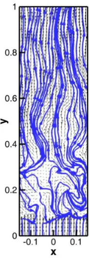
To have some preliminary idea about the flow structure in the measuring plane, an example of the instantaneous velocity field is presented in Fig. 2. To help with the vectors interpretation, the vector lines are added arbitrarily.
The flow-field could be divided into several parts along the y axis:
y (0;0.08): presence of the free stream, however above the surface. In this region the measuring plane is above the boundary layer, which is very thin here, less than 1 mm,
y (0.08;0.25): separation bubble with backward oriented flow,
y (0.25;1): normal streamwise flow, however perturbed.
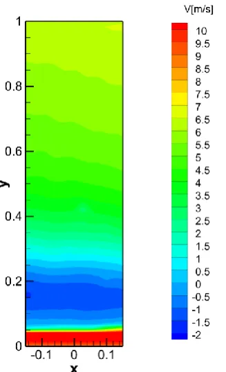
Separation of the flow is located very close to the leading edge, reattachment point is located at y = 0.25. This result is supported by the mean velocity vectors distribution in Fig. 3, colours represent velocity modulus.
Fig. 2. Instantaneous velocity vectors.
In Fig. 3 the vectors are coloured according to the local mean velocity magnitude (“Length”). Additional confirmation shows Fig. 4, where distribution of the streamwise mean velocity component V is shown. The backward flow region is in blue.
Fig. 4. Streamwise mean velocity component distribution.
Fig. 5. Sum of in-plane velocity components variances distribution.
The dynamic activity is quantified using the sum of velocity components variances, shown in Fig. 5.
The results indicates maximal dynamical activity within the separation bubble, especially the bubble leading edge in the plane of measurement is intensively changing its position.
To visualise possible vortical structures oriented in the z-direction perpendicular to the plate, the corresponding vorticity component has been evaluated. In Fig. 6 there is an example of distribution of the instantaneous vorticity component in z-direction.
Fig. 6. Instantaneous vorticity distribution.
Both positive and negative vorticity is present in the instantaneous field, structure is rather random, however the maximum magnitude indicates presence of waves in the velocity field – compare with Fig. 2.
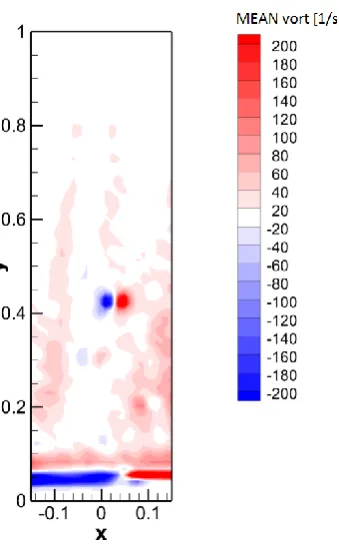
Statistical characteristics of the vorticity have been evaluated as well. In Figs. 7 and 8 distributions of the vorticity mean value and RMS are depicted respectively. The maximal vorticity activity is detected within the separation bubble and in close to the y = 0.4 the vortex couple of opposite sign has been detected. It will be subjected to further analysis in future.
Fig. 7. Mean vorticity distribution.
Fig. 8. Vorticity RMS distribution.
3.2 Dynamics
Dynamical analysis has been carried out using the POD method. As vortical structures are to be studied, the POD analysis has been applied both on velocity and vorticity fields. The POD method maximizes the analysed quantity variance, in the case of velocity this corresponds to kinetic energy (double), while for vorticity the half variance equals to enstrophy.
The region close to the leading edge has been excluded from the space domain for the analysis, as dynamics of separation bubble has not been in the scope of our interest. The area of interest is reduced for the study of dynamics, the range for dynamical analysis is defined as follows:
x
(-1.5;1.5), y
(0.15;1).3.2.1 Dynamics of velocity field
The dynamical analysis is applied on the velocity fields, the velocity POD modes nave been evaluated. Each mode is characterised by its energy. Distribution of the energy across the velocity POD modes is shown in Fig. 9 for the lowest 1000 modes, note that the vertical axis is log.
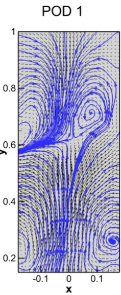
Fig. 9. Energy distribution across the velocity POD modes. In Fig. 9 there is the “Energy Fraction” indicating relative energy of a given POD mode and the “Accumulated Energy” which represents the energy contained in all modes with number lower and equal to the given mode. The Total Kinetic Energy (TKE) is considered to be 1. For example the 1st velocity POD mode contains 2.8% of the TKE, 10 first POD modes cover 20% and 100 modes about 67% of the TKE.
Fig. 10. Velocity POD mode No. 1, 2.8% TKE.
Fig. 11. Velocity POD mode No. 2, 2.6% TKE.
Fig. 12. Velocity POD mode No. 3, 2.4% TKE.
Fig. 14. Velocity POD mode No. 100, 0.23% TKE.
The typical dynamics of the velocity field is characterized by low-order modes, they consist of a small number of big vortices distributed in the velocity field. The vortices are located in the middle part of the plate chord.
The higher order velocity POD modes contain relatively small amount of TKE and they consist of a big number of small vortices distributed regularly in the whole domain.
3.2.2 Dynamics of vorticity field
The similar dynamical analysis is applied on the vorticity fields, the vorticity POD modes have been evaluated. However, there is a difference in the procedure, as now we work with scalar fields instead of vectors. Now, each mode is characterised by its enstrophy. Distribution of the enstrophy across the vorticity POD modes is shown in Fig. 15 for 1000 modes, the vertical axis is log. The figures on both “Enstrophy Fraction” and “Accumulated Enstrophy” are relative to the Total Enstrophy (TE).
The enstrophy of the 1st vorticity POD mode is about 1.05% of the TE, while 10 lowest order modes cover 9% and 100 modes 53% of the TE.
Fig. 15. Enstrophy distribution across vorticity POD modes. Examples of the vorticity POD modes topologies are to be shown in Figs. 16-20 representing the modes Nos. 1, 2, 3, 20 and 100 respectively. Distribution of the vorticity component in z direction, red – positive, blue – negative (clockwise).
Fig. 17. Vorticity POD mode No. 2, 1.03 TE.
Fig. 18. Vorticity POD mode No. 3, 1% TE.
Fig. 19. Vorticity POD mode No. 20, 0.71% TE.
The lower order vorticity POD modes (1, 2, 3) are typical with vortical activity organized in strips with streamwise direction. The strips are located close to the middle of the chord and are of alternating orientation.
The high order vorticity POD modes are characterized by more or less regularly distributed vorticity in spots of positive and negative vorticity.
4 Conclusions
Topology of the flow in the vicinity of suction surface of the flat plate in regular stream with angle of attack 7° was studied experimentally. Time resolved PIV method has been applied with measuring plane located close to the plate surface parallel to it. Detected velocity could be linked to skin friction on the suction surface of the plate.
Both velocity and vorticity fields have been explored using classical statistical methods and POD method. Typical vortical structures have been detected.
Acknowledgments
This work was supported by the Grant Agency of the Czech Republic, project No. 17-01088S.
References
1. J. Hoffman, C. Johnson, The Mathematical Secret of Flight, Normat 57, 4, pp.1–25, (2009)
2. J. Hoffman, C. Johnson, Resolution of d’Alembert’s paradox, J. Math. Fluid Mech., 12 (3), pp.321-334, (2010)
3. J.L. Lumley, The structure of inhomogeneous turbulent flows, Atm.Turb. and Radio Wave Prop., Yaglom and Tatarsky eds., Nauka, Moskva, pp. 166-178 (1967)
4. L. Sirovich, Turbulence and the dynamics of coherent structures. Quart. Appl. Math., 45, pp. 561-590 (1987)
5. V. Uruba, D. Pavlík, P.Procházka, V.Skála,
V. Kopecký, On 3D flow-structures behind an
inclined plate, EPJ Web of Conferences, 143, Article number 02137 (2017)
6. V. Uruba, Near Wake Dynamics around a Vibrating Airfoil by Means of PIV and Oscillation Pattern Decomposition at Reynolds Number of 65 000, Journal of Fluids and Structures, 55, pp. 372-383 (2015)