Parameter Estimation for an Allometric Food Web Model
H. T. Banks
∗, J. E. Banks
@, Riccardo Bommarco
+, Alva Curtsdotter
+,
Tomas Jonsson
+,×, and A. N. Laubmeier
∗∗
Center for Research in Scientific Computation,
North Carolina State University,
Raleigh, NC 27695
@Undergraduate Research Opportunities Center (UROC),
California State University, Monterey Bay,
Seaside, CA 93955
+Department of Ecology,
Swedish University of Agricultural Sciences,
Uppsala, Sweden SE-75007
×
School of Bioscience,
University of Sk¨
ovde,
Sk¨
ovde, Sweden SE-54128
May 29, 2016
Abstract
We present a preliminary attempt at applying an Allometric Trophic Network (ATN) model to single-season population data from agricultural fields. We describe the
pop-ulation dynamics of Rhopalosiphum padi, an aphid pest species, using predator-prey
1
Introduction
Against a backdrop of worldwide biodiversity decline, the growing awareness of our societal reliance on ecosystem services creates a need to understand how the provisioning of these services depends on biodiversity [12, 37]. Biodiversity (i.e., organisms) perform ecosystem functions. A subset of these functions are beneficial to humans and these are defined as ecosystem services [3]. Ecosystem services can be defined as final; these are the services we benefit from directly and include crop yields for food, fibre and bioenergy, wild fish and berries [4]. The final services are underpinned by intermediate services such as control of crop pests via predation by their natural enemies, crop pollination and nutrient cycling [4]. To conserve and manage ecosystem services we need to better understand how biodiversity and ecosystem services are linked [12].
From the recent decades of research in the fields of biodiversity-ecosystem functioning (BEF) and biodiversity-ecosystem services (BES), we have learned that both functioning and service provisioning generally exhibit a positive, but saturating, relationship to di-versity most often defined as the number of species in the community [12]. However, we have also learned that this is not always the case [22], and that we lack the mechanistic understanding of these relationships to predict when biodiversity will increase function-ing and service provisionfunction-ing, and when it will not. Furthermore, there is also uncertainty as to whether the positive BEF and BES relationship will hold up even as a general rule in a multi-trophic context, as our current understanding of these relationships is based almost exclusively on studies of single trophic levels (i.e., primary producers)(see [19]). A case in point is the ecosystem service of biological control of insect pests in agricul-tural crops, underpinned by the function of predation performed by the pest’s naagricul-tural enemies. Biological control inherently involves multiple trophic levels, and the effect of biodiversity on this ecosystem service is quite variable; both positive and negative relationships occur frequently ( [12] and references therein).
Biological control is a valuable ecosystem service; the insect-provided biocontrol ser-vices in the US alone are estimated to US 4.5 billion dollars annually [32]. But conven-tional farming often undercuts its potential through practices equally detrimental to the target pest as to its enemies [46,48,49,51]. There is therefore substantial societal interest in shaping agro-ecosystems so as to better support this service [10, 41, 50]. But our lack of mechanistic understanding of biological control in the field, and the predation that underpins it, makes this quite challenging. What we do know is that there are several, and sometimes opposing, mechanisms through which biodiversity can affect the level of biological control [12, 19, 31]. Complementarity and facilitation among predators will in-crease functioning and service levels with biodiversity, while competition and intra-guild predation will have the opposite effect. We are, however, not in a position where for a given predator-prey community we can predict which processes will dominate, and hence what the effect of biodiversity on biological control will be [12].
for the effect of biodiversity on biological control [12]. Furthermore, through the use of dynamical food web models (i.e., models of multi-species predator-prey population dynamics) the interplay between such opposing mechanisms could be investigated, and a more mechanistic understanding of the relation between biodiversity and the level of biological control could be gained. Ultimately, empirically informed dynamical food web models could become valuable tools for making quantitative predictions of biological control.
For dynamical food web models to fully achieve their potential, their usefulness in a real-world setting must be established. Dynamical food web modeling has long stayed within the realm of theoretical ecology, often applied to classical questions about the stability of ecosystems [11]. Mostly they have been used to model a kind of idealized ecosystem, the results from which are assumed to be generally applicable. It is only
recently, thanks to the advent of allometric (i.e., body-size based) parameterizations,
that dynamical food web models have been successfully applied to model the real dy-namics of specific ecosystems, such as the plankton community of Lake Constance, or experimental predator-prey microcosms [9, 26, 44]. The goal of these studies has been two-fold; by attempting to replicate observed population dynamics with a mechanistic model, the model can be validated at the same time as insight can be gained into the mechanisms governing the real population dynamics and the variation the model fails to capture may lead us to perceive additional mechanisms governing the real popula-tion dynamics. For example, the successful attempt to replicate the plankton dynamics of Lake Constance, highlighted the importance of the detrital loop and prey resistance for this specific system, while simultaneously demonstrating the usefulness of dynamical food web models in real-life applications [9].
So far, the attempts to model empirically observed food web dynamics have been very few, and have mostly been constrained to the highly controlled environment of a microcosm [26, 44]. In the one pioneering attempt to model the population dynamics of a natural food web, the observed dynamics were not for one specific year but an average across 10 years, in order to focus on general ecological processes rather than specific events (e.g., the year-specific weather) [9]. However, in order for dynamical food web modeling to become useful as a predictive tool for ecosystem services such as biological pest control, we need to quantitatively model and predict dynamics of predator prey dynamics under a range of conditions.
Here, we take a first step towards this goal: we attempt to replicate the observed population dynamics of an herbivorous pest species, subjected to predation from natural enemies, in 10 Swedish spring barley fields in 2011. The study system includes the focal
pest species, the bird-cherry oat aphid (Rhopalosiphum padi), a variety of its natural
The work presented here is the first step in an iterative modelling process [7], in which our first attempts with the inverse problems inform our future efforts in describ-ing the system of interest. These inverse problems are simply an attempt to minimize the distance between real observations and the proposed dynamics that model our system. In carrying out the inverse problems, we arrive at a set of parameters for a mathemat-ical model (in this case, the ATN model) that allow us to best-fit the observed data. However, the first attempt to solve an inverse problem naturally invites us to question the accuracy of the data, including the properties its observation errors might possess, as well as how much information about our system could be possibly represented in a given data set. In evaluating the performance of the inverse problems, we often find that the mathematical and/or statistical models require reformulation. Thus we usually must statistically address the nuances of inherent errors in data collection. Arriving at these statistical and mathematical model reformulations yields new inverse problems to solve, and so we repeat the modelling process until a sufficient theoretical framework has been developed to compare with experimental data. In this way, the inverse problems represent an experiment in themselves; we have hypothesized a mathematical and a sta-tistical model and seek to investigate their validity and shortcomings within the context of our study system.
2
Model and Data
In the following sections, we explain in detail the data collection and necessary data transformations, the mathematical model and its parameters, as well as the procedures involved in solving the inverse problem. Here, we briefly summarize the role of each of these components. The food web details the predator-prey interactions, as well as the taxonomic resolution of the mathematical model. The mathematical model (i.e., the ATN model) describes how the aphid population density develops over time, as a func-tion of a temperature dependent intrinsic rate of increase and predafunc-tion from the natural enemies. The empirically observed population densities of natural enemies and alterna-tive prey, together with their body masses, determine the strength of the predation. The empirically observed aphid population density is what the mathematical model should replicate, and we will employ inverse problem techniques to find the parameter values that optimize the mathematical model fit to this data. This optimization is described in terms of a cost function, which in turn is dictated by a choice of the statistical model. Prior to the optimization steps, a sensitivity analysis is performed to investigate which of the parameters to be estimated affect most the behaviour of the mathematical model.
2.1
Study system
The original purpose of the data collection was to study the biological control of aphids by natural enemies in spring barley fields. The study focused on the bird cherry-oat
aphid,Rhopalosiphum padi, a set of aphid predators (carabid and coccinellid beetles, and
province of Uppland, Sweden; five fields each of conventional and organic agriculture. The sampling design is paired, and the two fields in each conventional-organic pair are at most 1-2 kilometers apart. However, there was no significant effect of the management style on the biological control of the aphids [39], and therefore we do not consider this aspect here.
2.2
Food web structure
Each node in the food web corresponds to a taxonomic entity (e.g., species, genus, family, or order), and the links represent feeding interactions between these nodes. The food web was constructed using molecular gut content analysis (MGCA) of the predators. The predators were sampled in each field, using dry pitfall traps open for 24 hours on four sampling occasions (twice early in the season and twice late). The collected predators were identified to species and subjected to whole-body DNA extraction. Finally, the predators were screened for DNA of any of the prey categories (i.e., the food web nodes) using diagnostic multiplex PCR assays. Thus, the taxonomic resolution of the food web was determined by the resolution of the prey categories used in the MGCA. For a full description of i) the sampling procedure, see [42], and ii) the MGCA, see [47].
We used the MGCA data from all fields and the entire season to construct a bi-nary food web. All observed feeding events are represented by a link, regardless of the frequency of observation. We also pool the data across space and time, and so the resulting food web should be interpreted as showing the potential feeding interations
between nodes. The per capita interaction strengths are based on predator-prey body
mass rather than observation frequency; see the model equations given below in Section 2.3.
There are certain types of links that cannot be detected by the MGCA. Cannibalism cannot be detected, as the MGCA cannot discriminate between the DNA of the preda-tor individual and con-specific DNA in its gut. Similarly, the prey category “Other Carabid” cannot be detected in the carabid nodes (Bembidion, Harpalus, Poecilus, and Pterostichus), and the prey category “Other Spider” cannot be detected in the spider nodes (Linyphiidae, Lycosidae, and Tetragnathidae). Additionally, the nodes Tetrag-nathidae and Other Spider were not analyzed as predators in the MGCA. The results of the MGCA are given in Table 1.
Consumer Aphid Thrips Diptera Collem
b
ola
Earth
w
orm
Bem
bidion
Harpalus Po
ecilus
Pterostic
h
us
Other
Carabid
Lin
yphiidae
Lycosidae Tetragnathidae Other
Spider
Co
ccinella
Resource
Aphid * * * * * 1 1 1 1 1 1 1 * * 1
Thrips * * * * * 1 1 1 1 0 1 1 * * 1
Diptera * * * * * 1 1 1 1 1 1 1 * * 1
Collembola * * * * * 1 1 1 1 1 1 1 * * 1
Earthworm * * * * * 1 1 1 1 1 1 1 * * 1
Bembidion * * * * * * 1 1 1 1 1 1 * * 1
Harpalus * * * * * 1 * 1 1 1 1 1 * * 1
Poecilus * * * * * 1 1 * 1 1 1 1 * * 1
Pterostichus * * * * * 1 1 1 * 1 1 1 * * 1
Other Carabid * * * * * * * * * * 1 1 * * 0
Linyphiidae * * * * * 1 1 1 1 1 * 1 * * 0
Lycosidae * * * * * 1 1 1 1 1 1 * * * 0
Tetragnathidae * * * * * 0 1 1 1 1 1 1 * * 0
Other Spider * * * * * 1 1 1 1 1 * * * * 1
Coccinella * * * * * 1 1 1 1 1 0 1 * * *
Table 1: The incomplete interaction matrix for our system, where each column represents a
consumer node. If there is a 1 in the (i, j)th entry of the matrix, then node i is a resource for
nodej. If there is a * in the (i, j)th entry, then the gut content analysis did not provide data
Consumer Aphid Thrips Diptera Collem
b
ola
Earth
w
orm
Bem
bidion
Harpalus Po
ecilus
Pterostic
h
us
Other
Carabid
Lin
yphiidae
Lycosidae Tetragnathidae Other
Spider
Co
ccinella
Resource
Aphid 0 0 0 0 0 1 1 1 1 1 1 1 1 1 1
Thrips 0 0 0 0 0 1 1 1 1 0 1 1 1 1 1
Diptera 0 0 0 0 0 1 1 1 1 1 1 1 1 1 1
Collembola 0 0 0 0 0 1 1 1 1 1 1 1 1 1 1
Earthworm 0 0 0 0 0 1 1 1 1 1 1 1 1 1 1
Bembidion 0 0 0 0 0 1 1 1 1 1 1 1 1 1 1
Harpalus 0 0 0 0 0 1 1 1 1 1 1 1 1 1 1
Poecilus 0 0 0 0 0 1 1 1 1 1 1 1 1 1 1
Pterostichus 0 0 0 0 0 1 1 1 1 1 1 1 1 1 1
Other Carabid 0 0 0 0 0 1 1 1 1 1 1 1 1 1 0
Linyphiidae 0 0 0 0 0 1 1 1 1 1 1 1 1 1 0
Lycosidae 0 0 0 0 0 1 1 1 1 1 1 1 1 1 0
Tetragnathidae 0 0 0 0 0 0 1 1 1 1 1 1 1 1 0
Other Spider 0 0 0 0 0 1 1 1 1 1 1 1 1 1 1
Coccinella 0 0 0 0 0 1 1 1 1 1 0 1 0 1 1
Table 2: The interaction matrix for our system, where each column represents a consumer
node. If there is a 1 in the (i, j)th entry of the matrix, then nodei is a resource for node j.
2.3
Allometric Trophic Network (ATN) model
The aphid (R. padi) population densityN1(t) [ind1 m−2] is modelled dynamically using
the ATN model [44]
dN1
dt (t) =N1(t)
r(T(t))−
X
j∈C1
a1jNj(t)
1 +cjNj(t) +Pk∈RjakjhkjNk(t)
, (1)
with initial conditionN0
1. For allj6= 1, the population densityNj [indj m−2] is obtained
from experimental data (see 2.5 for details).
Here,r(T) [d−1] is the temperature dependent growth rate of the aphid,aij[m2d−1ind−j1]
is the attack rate of predatorj on preyi,cj [m2 ind−j1] is the coefficient of intra-specific
interference competition of the predator, andhij [d indj ind−i 1] is the handling time for
one individual of predator j to handle one individual of prey i. C1 is the set of nodes
that predate on the aphid, andRj is the set of nodes that are prey to predator j.
The constant parameters aij, hij and cj are body-size dependent, and are
aij =a0Wi1/4W
1/4
j
Wj/Wi
Ropt
e1−
Wj /Wi Ropt
φ
hij =h0(Wi/Wj)1/4
cj =c0Wj1/2.
(2)
Here, Wi [mg ind−i 1] and Wj [mg ind−j1] are the body masses of prey i and
preda-tor j, respectively, and Ropt [indi ind−j1] is the optimal predator-prey body mass
ra-tio. The parameters a0 [m2 d−1 mg−0.5 ind0i.25 ind
−0.75
j ], h0 [d ind
−0.75
i ind
−0.75
j ], and
c0 [m2 mg−0.5 ind−j0.5] are normalization constants and φ is a unitless width scaling
parameter. We estimate the parameter values of [a0,h0,c0,Ropt,φ] by carrying out an
inverse problem (see section 3 below for details).
2.4
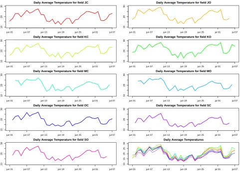
Temperature-dependent growth and temperature data
The intrinsic growth rate, r, of the aphids was modeled as a linear function of the field
temperatures,T(t):
r(T) =.024T −.089. (3)
The function T → r(T) depicted in Figure 1 was determined using a linear regression
of data on the intrinsic rate of increase of aphidsR. padi kept at different temperatures
(10-30°C) in the laboratory setting [18]. For the regression we further assumed that the
intrinsic rate of increase is 0 at 3°C.
●
●
●
●
●
5 10 15 20 25
0.0 0.1 0.2 0.3 0.4 0.5
Temperature
r
jun 01 jun 07 jun 13 jun 19 jun 25 jul 01 jul 07
10
20
30
Daily Average Temperature for field JC
Date
T
emper
ature (°C)
jun 01 jun 07 jun 13 jun 19 jun 25 jul 01 jul 07
10
20
30
Daily Average Temperature for field JO
Date
T
emper
ature (°C)
jun 01 jun 07 jun 13 jun 19 jun 25 jul 01 jul 07
10
20
30
Daily Average Temperature for field KC
Date
T
emper
ature (°C)
jun 01 jun 07 jun 13 jun 19 jun 25 jul 01 jul 07
10
20
30
Daily Average Temperature for field KO
Date
T
emper
ature (°C)
jun 01 jun 07 jun 13 jun 19 jun 25 jul 01 jul 07
10
20
30
Daily Average Temperature for field MC
Date
T
emper
ature (°C)
jun 01 jun 07 jun 13 jun 19 jun 25 jul 01 jul 07
10
20
30
Daily Average Temperature for field MO
Date
T
emper
ature (°C)
jun 01 jun 07 jun 13 jun 19 jun 25 jul 01 jul 07
10
20
30
Daily Average Temperature for field OC
Date
T
emper
ature (°C)
jun 01 jun 07 jun 13 jun 19 jun 25 jul 01 jul 07
10
20
30
Daily Average Temperature for field SC
Date
T
emper
ature (°C)
jun 01 jun 07 jun 13 jun 19 jun 25 jul 01 jul 07
10
20
30
Daily Average Temperature for field SO
Date
T
emper
ature (°C)
jun 01 jun 07 jun 13 jun 19 jun 25 jul 01 jul 07
10
15
20
25
30
Daily Average Temperatures
Date
T
emper
ature (°C)
Figure 2: Daily average temperatures T(t) with linear interpolation plotted as a function of time.
2.5
Population densities
Abundance data were collected using different techniques and frequency for aphids, other plant-dwelling arthropods, soil organisms, and ground-dwelling predators. For use in the population model, the abundance data were converted to population densities [individuals/m2]. The conversion depends on the technique with which the node was sampled.
Aphids (R. padi) were sampled 5-6 times in each field, about once a week, during the 6
week long study period. At each field and time, aphids were counted on 100 barley tillers (except at time 3 in field JC: 65 tillers) by randomly choosing 10 batches of 10 consecutive
tillers. All batches were ≥ 10m from the field border. To convert the abundance to
density N, we used Ns =AsB, where As is the abundance [aphids/tiller] at sampling
occasions, and B is the barley tiller density [tillers/m2]. We used B = 411 [42].
of colonization, detection of such a low level immigrant abundance is not surprising (observation error, and immigration is a continuous process while we’re sampling in discrete time) so we adjusted/seeded it with the min detectable density. We defined the
minimum detectable density as 4.1[aphids/m2] (i.e., a single aphid across the 100 tillers).
In addition to being shifted, the aphid time series were also truncated. The growth rate of the aphids depends not only on the temperature, but also on the maturation stage of the crop [30]. Here, we have simplified this relationship by assuming the growth rate is not affected until a critical crop maturation stage is reached, after which the growth rate plummets. From this point forward our model cannot be expected to capture the aphid dynamics. To carry out the inverse problems, we therefore truncated the aphid time series by excluding data points after the date the critical crop maturation stage was reached. The crop maturation stage of each field was estimated weekly, by classing 20 barley plants according to the BBCH-scale for cereals. The fields were defined as having reached the critical stage when at least 25% of the plants had reached stage 50 or higher [30].
Other plant-dwelling arthropods (Thrips, Diptera, and Coccinella) were sampled 2-4 times during the study period, with 1-4 weeks between sampling occasions. At each field and time, these arthropds were collected in 50 sweeps with a sweepnet. We converted
to density N(t) with the relationship Ni,s =Ai,s/an, where Ai,s is the total number of
individuals of taxon icollected at sampling occasionswith then sweeps, andan is the
area covered by thensweeps. We calculatean as
an=nfcπ((La+fhLh+dnet)2−(La+fhLh)2),
wheren is the number of sweeps, fc is the fraction of a circle that a sweep constitutes,
La is the length of the arm of the person doing the sampling, Lh is the length of the
sweepnet handle,fh is a factor taking into account the effective reduction of the sweep
circle diameter caused by the handle being held at some angle towards the ground and
at some length in on the handle, anddnet is the diameter of the net itself. Here, we used
n= 50, fc= 0.29 (estimating forehand and backhand sweep to 1/3 and 1/4 of a circle,
respectively),La= 0.65m,fh = 1/3,Lh= 0.85m, and dnet = 0.353m.
Soil organisms (Collembola and Earthworm) were sampled twice, approximately 4
weeks apart, using soil samples: 6 samples of diameter 0.05[m] for springtails and 4
samples of diameter 0.25[m] for earthworms at each field and time. We convert to density
N(t) using Ni,s = Ai,s/asampler, where Ai,s is the abundance [individuals/sample] of
taxon i, andasampler is the area of soil sampler at sampling occasion s.
Ground-dwelling predators (Bembidion, Harpalus, Poecilus, Pterostichus, Other Cara-bid, Linyphiidae, Lycosidae, Tetragnathidae, and Other Spider) were sampled using wet pitfall traps (6 traps/field). The traps were left open for the entire study period, and emptied 5 times (approximately once a week). For the ground-dwelling predators, sam-pled with pitfall traps, the conversion to population densities involved first correcting for body-mass bias in the pitfall catches, and then converting the corrected catch to density. There is a known size-bias in abundance data obtained through pitfall catches [2].
Although allometric theory predicts a negative 34 relationship between body mass and
We assume that abundance data ˜nji, obtained at time tj for the ith species, should
follow the allometric relationship
˜
nji =Cexp
−3
4(mi−M)
,
for mi the species body mass and M the average body mass over all species. Using a
log-linear regression over all speciesiand timestj, we obtain a fit to data that does not
follow the−34 law, given by
˜
nji =Cexphf(mi−M) +ji i
.
Here, ji is the error in abundance observation and C, f are constants obtained by
regression on the data. We use the constant C and errors ji to obtain the “unbiased”
abundancesnji that follow the −3
4 relationship,
nji =Cexp
−3
4(mi−M) +
j i
.
After we obtain the unbiased abundance data, we convert to a density by, for each field and sampling occasion, calculating the average daily catch (i.e., the total catch divided by the number of days since the trap was last emptied), and assuming that each
day the trap catches individuals from an area ofπ1.52m2 [54].
The composition of the predator community differs substantially between fields, both in terms of how evenly the biomass is distributed across the consumer nodes and in terms of the identity of the dominating node. There seems to be a spatial correlation, giving similar compositions within each conventional-organic field pair. The fields also differ in their body mass distribution, as seen in Figure 35. Although all fields exhibit long tails, with large predators having low biomass, there is variation both with regards to which body mass is dominating the biomass abundance, and how strongly so.
2.6
Body masses
The calculation of node body mass depends on the taxonomic resolution in the abun-dance data. If the resolution of the abunabun-dance data is the same as that of the node (i.e., nodes Aphid, Thrips, and Earthworm), the node is assigned a body mass which does not vary across fields. However, if the resolution of the abundance data is higher than that of the node (i.e., all the predator nodes, Collembola, and Diptera), the assigned body mass will vary across fields, as the species composition of a node is unique to the field in which the abundance data was collected. In these cases, we take a weighted average of the constituting species’ body masses to compute the effective mass of the node. The weight given to each species’ mass is the species’ relative contribution to node abundance
over the entire season. That is, for a node withm constituting species andspopulation
samples, the effective massW of the node is
W =
m X
i=1
wi
1
n
m X
j=1
nji
Ps
j=1n
j i
forwithe body mass of theith species andnji the numerical abundance of theithspecies
at observation j. For nodes observed with pitfall traps, we use the unbiased abundance
data. The node body masses used in the simulations are given in Table 3.
Node Body mass (mg)
Aphid 0.59
Thrips 0.23
Diptera 26.674-29.687
Collembola 0.0015-0.0021
Earthworm 155
Bembidion 1.276-1.606
Harpalus 53.368-61.770
Poecilus 44.422-45.770
Pterostichus 85.179-103.960
Other Carabid 2.283-21.3030
Linyphiidae 1.036-1.638
Lycosidae 4.802-16.490
Tetragnathidae 1.910-2.263
Other Spider 3.938-31.900
Coccinella 4.470-20.780
Table 3: Node body mass in milligram fresh weight. For nodes with field-specific body mass, the range across fields is given.
For node Aphid we used the adult body mass of asexually reproducing individuals of R. padi reported in [13].
For node Thrips (Thysanoptera), the species composition is unknown and we there-fore assumed that the node is composed in equal parts of four species common in spring
barley in Sweden: Limothrips denticornis,Thrips augusticeps,Frankliniella tenuicornis,
and Anaphotrips obscurus. Body lengths of these species found in [29] were converted to dry weight using a length-weight relationship for Thysanoptera [24]. Dry weight was converted to fresh weight using a factor 2.3 (see calculation of carabid body mass below). The Diptera were determined to family or suborder: Syrphidae, other Brachycera, and Nematocera. We assumed the following body lengths: Syrphidae 10 mm [14], other Brachycera 10 mm and Nematocera 12 mm [24]. Dry weight was calculated from length-weight relationships given in [24] and converted to fresh length-weight using the factor 2.3.
The Collembola were determined to order: Arthropleona and Symphypleona. To calculate the body mass of these groups, we used data on species composition and body
length from barley fields in the province of V¨asterg¨otland, Sweden (Laura Riggi,
unpub-lished data). Dry weight was caluclated from length-weight relationships for collembolan families in [38], and converted to fresh weight using the factor 2.3.
The node Earthworm (Lumbricidae) was assigned a body mass corresponding to the average (across species and three years) fresh weight of individuals in the earthworm community of a winter cereal field on Ireland [17].
The coccinellids were not categorized by species but by developmental stage: adults, and larvae. We calculate adult coccinellid body mass as the average of two species
small, Propylea quatuordecimpunctata. The body mass of each species was averaged across multiple sources: [26] (fresh weight), APPEAL (Kerstin Reifenrath, unpublished data) and [25] (dry weights converted to fresh weight by the factor 2.3). Larval weight was assumed to be 21% of adult body mass, based on observed adult-larvae body mass ratio (Kerstin Reifenrath, personal communication).
Carabids (nodes Bembidion, Harpalus, Poecilus, Pterostichus and Other Carabid) were determined to species. We converted carabid body lengths [21] [53, and references therein] to dry weight using a length-weight relationship for Carabidae [28]. Dry weights were converted to fresh weight using a factor of 2.3, which is the fresh-to-dry-weight ratio between the weights from the length-dry weight and length-fresh weight relationships for carabids in [43].
Spiders (nodes Linyphiidae, Lycosidae, Tetragnathidae and Other Spider) were de-termined to species if adult, and to genus or family if subadult or juvenile. Body lengths were taken from [33–36]. Juveniles were assumed to be 25% the size of adults and subadualts were assumed to have the same size as adults (Gerard Malsher, personal
communcation). Body lengths were converted to fresh weights using family-specific
length-weight relationships [20]. For the few species belonging to families not covered by [20], we used a general length-weight relationship for spiders from the same paper.
3
Inverse Problems
3.1
Ordinary Least Squares
Given the dynamical system (1) from section 2.3
dN1
dt =g(t, N, q),
with unknown parameters q= [a0, Ropt, φ, h0, c0, N10], we assume that we have
observa-tions of the form
N1j =f(tj, q0) +j.
That is, we assume an absolute error statistical model for the observations.
Here, f(t, q) = N1(t, q) is the solution of the dynamical system (1) and we assume
there is some nominal parameter set q0 that describes our system, with observation
errorsj. We assume that thej are constant over longitudinal data. Then the ordinary
least squares (OLS) is an appropriate cost criteria [7, 8] to use for solution to the inverse problems given by
qOLS = arg min
q s X
j=1
h
N1j−f(tj, q)
i2
.
For each field, we have data{nj1}, and so the realization of the OLS solution is
ˆ
q = arg min
q s X
j=1
h
nj1−f(tj, q)
i2
.
We seek the OLS realizations that minimize the cost functional in MATLAB, using
the minimizer lsqnonlin and stiff ODE solver ode23s. As initial parameter guess we
[a0 = 0.31, Ropt= 128, φ= 0.9744, h0 = 0.08, c0 = 0.21], and for the initial density,N10, we use the first aphid data point.
In this preliminary proof-of-concept presentation of a modeling approach to food-webs, we have chosen to use a least squares cost formulation which is equivalent to tacitly assuming that the measurement or observation error (i.e., the error in the statis-tical model) is absolute error [7, 8]. In future efforts we plan to further investigate the statistical processes involved in collection of abundance data in typical food web stud-ies. This of course is necessary before any uncertainty investigations (e.g., parameter uncertainty bounds) can be attempted since uncertainty bounds depend (in either a fre-quentist or Bayesian treatment) [7, 45] on the statistical form of the observation process. Moreover, the information content aspects of data sets for these problems depend on the correctness of both the mathematical and statistical models [7] in order to pursue such investigations [5, 6].
3.2
Sensitivity Analysis
It is of interest to determine the parameters which we can best estimate in the inverse problem, especially with the sparse data we are using. The sensitivity to parameters
S= ∂N1
∂q is described by the sensitivity equations,
dS dt =
∂g ∂N1
S+∂g
∂q
whereS(0) = 0.
We can analytically compute the partial derivatives,
∂g ∂N1
=r(t)−X
j∈C1
a1jNjFj(1−N1a1jh1jFj),
∂g
∂q =−N1
X
j∈C1
Nj
∂a1j
∂q Fj+a1j ∂Fj
∂q
,
where we calculate ∂Fj
∂q forc0,h0, andqa=a0, φ, Ropt to be
∂Fj
∂qa
=−Fj2 X
k∈Rj
∂akj
∂qa
hkjNk,
∂Fj
∂h0
=−Fj2 X
k∈Rj
akj
∂hkj
∂h0
Nk,
∂Fj
∂c0
=−Fj2∂cj ∂c0
For each parameter we have the following derivatives:
∂aij
∂a0
=Wi1/4Wj1/4
Wi/Wj
Ropt
e1−
Wi/Wj Ropt
φ
∂aij
∂Ropt
=aij
φ
Ropt2 (Wi/Wj −Ropt) ∂aij
∂φ =aij
1−Wi/Wj
Ropt
+ ln
Wi/Wj
Ropt
∂hij
∂h0
= (Wi/Wj)1/4
∂cj
∂c0
=Wj1/2
and so the solutions to the sensitivity equations can be readily obtained in MATLAB,
also using the stiff ODE solverode23s. These are plotted in the Results section below.
4
Results
4.1
Empirical patterns
Before the critical plant maturation stage, the observed aphid population trajectories follow two general patterns, which we will later show have a bearing on how well the model succeeds in replicating the data. In one set of fields (MC: Fig. 12, MO: Fig. 14, OC: Fig. 16, and SO: Fig. 22) the aphid population shows an unceasing increase over time. In the remaining fields, the aphid population experiences one or more population crashes, after which the population recovers.
The initial population increase observed in some fields is so sharp as to warrant an examination of whether the population growth implied by the data is ecologically reasonable. To this purpose we applied a purely exponential single-species model,
dN1
dt =N1r(T).
This subset of the full model uses the same intrinsic rate of increase, r(T), and the
same starting density, N10. From the comparison between the single-species model and
the data, we can conclude that the in-field aphid population increase generally matches, or is slower, than expected from the exponential growth (Figs. 4, 6, ..., 22). Thus, in general the observed population increases are within ecologically reasonable limits. The only exception is the field JC. There could be several reasons for this; the intrinsic rate of increase is underestimated, there is substantial immigration, or sampling error (i.e., underestimation of the early population size, and/or overestimation of the peak population size).
The intrinsic rate of increase r(T) we use here is measured under lab conditions.
is not the case, we suggest that the lab estimation of the intrinsic rate of increase, is valid as a general approximation of the in-field rate.
All aphid populations are started by winged individuals immigrating into the barley fields. Here, we have made the simplifying assumption that the immigration phase is not overlapping with the population growth phase. Large violations of this assumption could lead to several problems, e.g., making the conclusions above about the intrinsic rate of increase erronous, and underestimation of the predation pressure in the full model. However, the very low proportions of winged individuals except for the first timestep (Fig. 3), leads to the conclusion that our assumption is not violated, and that the exclusion of immigration from the model formulation is justified. With regard to the field JC, in which the observed population trajectory overshoots the single-species model, the complete absence of winged individuals at the population peak makes immigration unlikely as the major driver of it.
Another possibility for the surprising model undershoot in field JC, is that the data is incorrect. The spatial distributon of aphids in a field is patchy; this makes population density estimates more difficult than if the spatial distribution had been homogenous, and particularly so at low population densities. This means that, despite the larger error bars for high population densities, the lower population estimates are likely fraught with a larger uncertainty. But for field JC, a tenfold underestimation of the actual density at the preceding time point would have been required for the peak to have been achieved without immigration and with the lab estimated rate of increase; such a large underestimation of the density is unlikely.
Field JC Sampling points Fr action 0.0 0.4 0.8
1.2 0 3 846 317 462 103
Field JO Sampling points Fr action 0.0 0.4 0.8
1.2 0 7 172 81 350 429
Field KC Sampling points Fr action 0.0 0.4 0.8
1.2 3 6 27 23 47 147
Field KO Sampling points Fr action 0.0 0.4 0.8
1.2 0 2 335 239 626 56
Field OC Sampling points Fr action 0.0 0.4 0.8 1.2 Winged 0
125 440 1963 399
Field OO Sampling points Fr action 0.0 0.4 0.8
1.2 0 35 18 34 14
Field SC Sampling points Fr action 0.0 0.4 0.8
1.2 1 15 29 51 1 48
Field SO Sampling points Fr action 0.0 0.4 0.8
1.2 1 175 471 701 2539 1165
Field MC Sampling points Fr action 0.0 0.4 0.8
1.2 2 42 120 321 2
Field MO Sampling points Fr action 0.0 0.4 0.8
1.2 1 148 651 1384 8
Figure 3: Proportion of winged (dark grey) and unwinged (light grey) aphids. Numbers above bars show total aphid count on the 100 tillers (for field JC, time 3, 65 tillers).
4.2
Results of the Inverse Problem and Sensitivity
Analy-sis
The results of the OLS minimization for each of the 10 fields are given in Table 4.2. We
rank the fields in decreasing size of the adjusted coefficient of determination, ¯R2, [27,
p.226] which is given by
¯
R2 = 1− 1− JOLS
Ps
j=1(n
j
1−n¯1)2
!
s−1
p−1
where ¯n1 is the mean of the aphid population data andp= 6 is the number of estimated
parameters.
Note that in Fields JC, MO, and SO, we haveROP T <1. SinceROP T is the optimal
predator-prey body mass ratio, we would not expect these values to fall below one.
Additionally, in field OO, the least squares solution takesφ= 0 and in fields JC and KO
the estimated value of φis close to 0. This results in a reduction of the ATN model to
a case where every predator attack is successful and increases the success rate for prey with a size not equal to the optimal mass. In field OO, the least squares solution takes
h0 = 0 and in fields KC and MC the estimated value of h0 is close to 0. This yields a
high prey densities and that abundance of alternative prey has no effect on the predation rate on the aphids. Because these parameters must be close to zero to generate aphid dynamics that are non-exponential, we conclude that the model does not currently have sufficient aphid mortality to match the slow growth rate of the population seen in the data. The other OLS parameter values fall within physically reasonable ranges.
Field R2 JOLS a0 Ropt φ h0 c0 N10
MC 0.94487 9.41×10⁴ 1.4075 2.9499 1.7739 0.0006 0.0034 0.9988
MO 0.82269 5.85×10⁶ 1.3382 0.0035 1.1083 0.1655 0.1807 1.0005
KO 0.75117 1.44×10⁶ 0.1206 111.21 0.0001 0.0003 0.3076 1.093
JO 0.71359 5.11×10⁵ 0.5396 1.0131 0.3167 0.1558 0.1885 1
OO 0.59907 9.21×10³ 0.1 259.56 0 0 0.0006 0.9854
KC 0.17699 2.21×10⁴ 0.3028 842.16 0.0734 0.0798 0.2083 1
OC -0.30973 6.96×10⁷ 5.3371 7.5993 1.1153 0.0086 0 1.003
SC -0.67343 6.34×10⁴ 1.3306 7.9432 0.4975 0.0347 0.2023 1
JC -0.51275 3.13×10⁷ 0.888 0.6357 0.0003 0.0021 0.9569 1.0001
SO -1.3242 2.05×10⁸ 7.8578 0.8159 0.271 0.1703 0.2606 0.9744
Table 4: Realizations of the OLS minimization for all 10 fields of data.
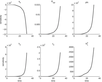
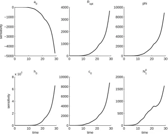
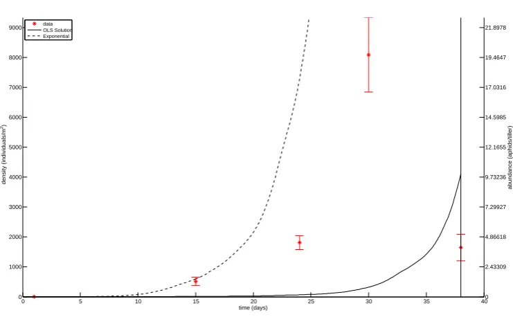
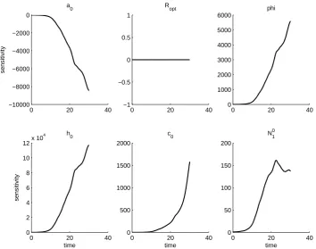
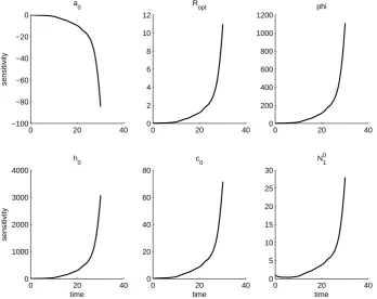
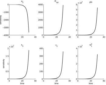
In Figures 4 to 23, we plot the OLS solution to the inverse problem as well as the solutions to the sensitivity equations for each field. When plotting aphid population dynamics, we indicate the solution to the inverse problem with a solid line. We plot with a dashed line the forward solution of the purely exponential population model discussed in Section 4.1. We note that in several of the fields (with the exception of fields JC, KO, MC, and OO in Figures 4, 10, 12, and 18 respectively), the solution to the inverse problem also appears exponential in nature, although with a slower growth rate than when predation is ignored.
In fields where the aphid population increases in time (fields MO and SO) or has population crashes on a sufficiently low scale to possibly be an artifact of measurement error (fields JO and KC), the OLS solution often underestimates the aphid population at early times and more closely follows the latest data point. This behaviour is likely driven by the choice of an OLS formulation for the inverse problem. Because we minimize absolute error and the population grows exponentially, the solution stays close to the high final data points and is not greatly penalized for undershooting the intermediate data points. However, the growth rate is lower than indicated in the majority of the data.
crashes in both the early and late parts of the season, and the OLS solution exhibits both of the aforementioned behaviors, ignoring the early aphid peak and running through the middle of the remaining population levels.
The success of the model to replicate the aphid dynamics thus varies substantially. The main failure of the model is that it cannot produce the aphid declines we see in several of the fields; clearly, the model lacks some critical process which can induce substantial but time limited mortality. The purely body-size-based predation of the ATN model cannot reproduce this pattern, at least given the observed predator densities. Comparing the single species model to the ATN model, does however show that predation can explain a large share of the aphid mortality; in the absence of predation, the aphid numbers soar to unrealistic heights. However, as the predation is the only possible source of mortality in the current model formulation, the optimization process involved in the inverse problem will strive to attribute as much mortality as possible to the predation. Therefore, we cannot conclude that body-size-based predation really accounts for this large a share of the aphid mortality, but we can conclude that it has the potential to do so.
We further note that the solutions to the sensitivity equations vary between fields. This is first a result of the sensitivity equations being a local analysis, and so the sensi-tivity of the aphid population to each parameter is only given at the parameter values obtained from the OLS procedure. However, even if the same set of parameters is used in each field, the solutions to the sensitivity equations will vary between fields. In fact, the parameter set which minimizes the OLS cost for one field can result in an intractable
system for ode23sto solve in a different field. The input of population densities for all
non-aphid nodes changes between fields, which has a significant effect on population dynamics. The interactions in the ATN model also depend on the body mass of each node, which is calculated using population data unique to each field. In general, we find
that the aphid population is least sensitive to parameterRopt and initial populationN01.
The aphid population is generally most sensitive to φand h0, but sensitivity toa0 and
c0 varies across fields.
Field Data Trajectory Model Trajectory Fit Category
MC Simply increasing non-exponential Averaging
MO Simply increasing Exponential Undershooting
SO Simply increasing Exponential Averaging
JO Increasing, low variability Exponential Undershooting
KC Increasing, low variability Exponential Undershooting
OC Increasing, late crash Exponential Averaging
SC Increasing, late crash Exponential Averaging
JC Variable Non-exponential Misses Peak, Averaging
KO Variable Non-exponential Misses Peak
OO Variable Non-exponential Averaging
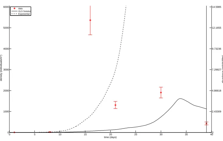
0 5 10 15 20 25 30 35 40 0
1000 2000 3000 4000 5000 6000
time (days)
density (individuals/m
2)
data OLS Solution Exponential
0 2.43309 4.86618 7.29927 9.73236 12.1655 14.5985
abundance (aphids/tiller)
Figure 4: OLS estimation for parameters in field JC. Data is plotted with star markers and 2SE errrorbars, and the OLS solution is plotted with a solid line. The solution obtained without predation is plotted with a dashed line. The cutoff date for the aphid data is indicated with a vertical line.
0 20 40
−8000 −6000 −4000 −2000 0
sensitivity
a 0
0 20 40
0 2 4 6 8
R opt
0 20 40
0 1 2 3 4x 10
5 phi
0 20 40
0 2 4 6 8x 10
6
time
sensitivity
h 0
0 20 40
0 1000 2000 3000 4000 5000 6000
time c
0
0 20 40
0 1000 2000 3000 4000
time N
1 0
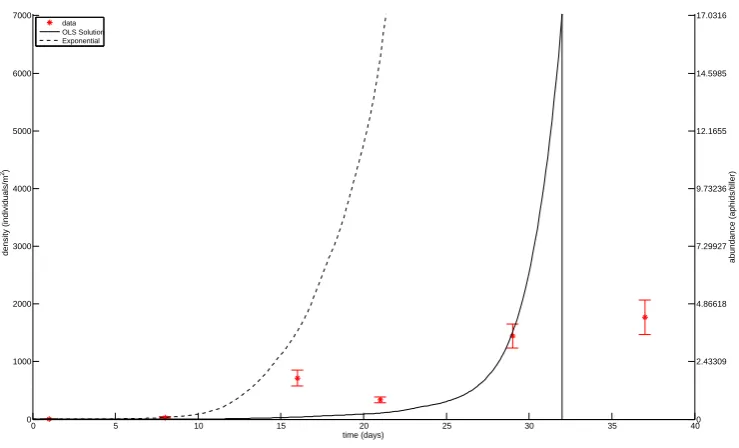
0 5 10 15 20 25 30 35 40 0
1000 2000 3000 4000 5000 6000 7000
time (days)
density (individuals/m
2)
data OLS Solution Exponential
0 2.43309 4.86618 7.29927 9.73236 12.1655 14.5985 17.0316
abundance (aphids/tiller)
Figure 6: OLS estimation for parameters in field JO. Data is plotted with star markers and 2SE errrorbars, and the OLS solution is plotted with a solid line. The solution obtained without predation is plotted with a dashed line. The cutoff date for the aphid data is indicated with a vertical line.
0 10 20 30 −3000
−2500 −2000 −1500 −1000 −500 0
sensitivity
a0
0 10 20 30 0
500 1000 1500 2000 2500 3000
Ropt
0 10 20 30 0
0.5 1 1.5 2 2.5
3x 10
4 phi
0 10 20 30 0
1 2 3 4x 10
4
time
sensitivity
h0
0 10 20 30 0
1000 2000 3000 4000 5000 6000
time c0
0 10 20 30 0
1000 2000 3000 4000
time N10
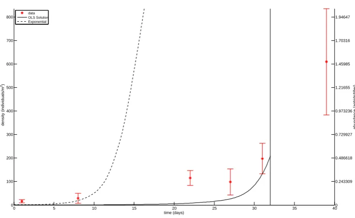
0 5 10 15 20 25 30 35 40 0
100 200 300 400 500 600 700 800
time (days)
density (individuals/m
2)
data OLS Solution Exponential
0 0.243309 0.486618 0.729927 0.973236 1.21655 1.45985 1.70316 1.94647
abundance (aphids/tiller)
Figure 8: OLS estimation for parameters in field KC. Data is plotted with star markers and 2SE errrorbars, and the OLS solution is plotted with a solid line. The solution obtained without predation is plotted with a dashed line. The cutoff date for the aphid data is indicated with a vertical line.
0 20 40
−200 0 200 400 600 800
sensitivity
a0
0 20 40
0 0.02 0.04 0.06 0.08 0.1
Ropt
0 20 40
0 1 2 3 4x 10
4 phi
0 20 40
0 1000 2000 3000 4000 5000
time
sensitivity
h0
0 20 40
0 200 400 600 800 1000
time c0
0 20 40
0 50 100 150
time N10
0 5 10 15 20 25 30 35 40 0
500 1000 1500 2000 2500 3000 3500
time (days)
density (individuals/m
2)
data OLS Solution Exponential
0 1.21655 2.43309 3.64964 4.86618 6.08273 7.29927 8.51582
abundance (aphids/tiller)
Figure 10: OLS estimation for parameters in field KO. Data is plotted with star markers and 2SE errrorbars, and the OLS solution is plotted with a solid line. The solution obtained without predation is plotted with a dashed line. The cutoff date for the aphid data is indicated with a vertical line.
0 20 40
−12 −10 −8 −6 −4 −2
0x 10 4
sensitivity
a 0
0 20 40
0 0.005 0.01 0.015
R opt
0 20 40
0 2 4 6 8 10x 10
4 phi
0 20 40
0 2 4 6 8x 10
5
time
sensitivity
h 0
0 20 40
0 0.5 1 1.5 2 2.5x 10
4
time c
0
0 20 40
0 500 1000 1500 2000 2500 3000
time N
1 0
0 5 10 15 20 25 30 35 40 0
500 1000 1500
time (days)
density (individuals/m
2)
data OLS Solution Exponential
0 1.21655 2.43309 3.64964
abundance (aphids/tiller)
Figure 12: OLS estimation for parameters in field MC. Data is plotted with star markers and 2SE errrorbars, and the OLS solution is plotted with a solid line. The solution obtained without predation is plotted with a dashed line. The cutoff date for the aphid data is indicated with a vertical line.
0 10 20 30 −5000
−4000 −3000 −2000 −1000 0
sensitivity
a 0
0 10 20 30 0
1000 2000 3000 4000
R opt
0 10 20 30 0
2000 4000 6000 8000 10000
phi
0 10 20 30 0
2 4 6 8x 10
5
time
sensitivity
h 0
0 10 20 30 0
2000 4000 6000 8000 10000
time c
0
0 10 20 30 0
500 1000 1500 2000
time N
1 0
0 5 10 15 20 25 30 35 40 0
1000 2000 3000 4000 5000 6000 7000 8000 9000
time (days)
density (individuals/m
2)
data OLS Solution Exponential
0 2.43309 4.86618 7.29927 9.73236 12.1655 14.5985 17.0316 19.4647 21.8978
abundance (aphids/tiller)
Figure 14: OLS estimation for parameters in field MO. Data is plotted with star markers and 2SE errrorbars, and the OLS solution is plotted with a solid line. The solution obtained without predation is plotted with a dashed line. The cutoff date for the aphid data is indicated with a vertical line.
0 10 20 30 −15000
−10000 −5000 0
sensitivity
a 0
0 10 20 30 −1
0 1 2 3x 10
8 R opt
0 10 20 30 0
1 2 3 4x 10
4 phi
0 10 20 30 0
1 2 3 4 5 6x 10
4
time
sensitivity
h 0
0 10 20 30 0
0.5 1 1.5 2 2.5x 10
4
time c
0
0 10 20 30 0
2000 4000 6000 8000 10000
time N
1 0
0 5 10 15 20 25 30 35 40 0
1000 2000 3000 4000 5000 6000 7000 8000 9000
time (days)
density (individuals/m
2)
data OLS Solution Exponential
0 2.43309 4.86618 7.29927 9.73236 12.1655 14.5985 17.0316 19.4647 21.8978
abundance (aphids/tiller)
Figure 16: OLS estimation for parameters in field OC. Data is plotted with star markers and 2SE errrorbars, and the OLS solution is plotted with a solid line. The solution obtained without predation is plotted with a dashed line. The cutoff date for the aphid data is indicated with a vertical line.
0 20 40
−8000 −6000 −4000 −2000 0
sensitivity
a 0
0 20 40
0 1000 2000 3000 4000 5000 6000
R opt
0 20 40
0 2 4 6 8 10x 10
4 phi
0 20 40
0 2 4 6 8 10x 10
5
time
sensitivity
h 0
0 20 40
0 0.5 1 1.5
2x 10 4
time c
0
0 20 40
0 2000 4000 6000 8000
time N
1 0
0 5 10 15 20 25 30 35 40 0
20 40 60 80 100 120 140 160 180
time (days)
density (individuals/m
2)
data OLS Solution Exponential
0 0.0486618 0.0973236 0.145985 0.194647 0.243309 0.291971 0.340633 0.389294 0.437956
abundance (aphids/tiller)
Figure 18: OLS estimation for parameters in field OO. Data is plotted with star markers and the OLS solution is plotted with a solid line. The solution obtained without predation is plotted with a dashed line. The cutoff date for the aphid data is indicated with a vertical line.
0 20 40
−10000 −8000 −6000 −4000 −2000 0
sensitivity
a 0
0 20 40
−1 −0.5 0 0.5 1
R opt
0 20 40
0 1000 2000 3000 4000 5000 6000
phi
0 20 40
0 2 4 6 8 10 12x 10
4
time
sensitivity
h 0
0 20 40
0 500 1000 1500 2000
time c
0
0 20 40
0 50 100 150 200
time N
1 0
0 5 10 15 20 25 30 35 40 0
50 100 150 200 250 300
time (days)
density (individuals/m
2)
data OLS Solution Exponential
0 0.121655 0.243309 0.364964 0.486618 0.608273 0.729927
abundance (aphids/tiller)
Figure 20: OLS estimation for parameters in field SC. Data is plotted with star markers and the OLS solution is plotted with a solid line. The solution obtained without predation is plotted with a dashed line. The cutoff date for the aphid data is indicated with a vertical line.
0 20 40
−100 −80 −60 −40 −20 0
sensitivity
a0
0 20 40
0 2 4 6 8 10 12
Ropt
0 20 40
0 200 400 600 800 1000 1200
phi
0 20 40
0 1000 2000 3000 4000
time
sensitivity
h0
0 20 40
0 20 40 60 80
time c0
0 20 40
0 5 10 15 20 25 30
time N10
0 5 10 15 20 25 30 35 40 0
0.5 1 1.5 2 2.5 3 3.5
x 104
time (days)
density (individuals/m
2)
data OLS Solution Exponential
0 12.1655 24.3309 36.4964 48.6618 60.8273 72.9927 85.1582
abundance (aphids/tiller)
Figure 22: OLS estimation for parameters in field SO. Data is plotted with star markers and the OLS solution is plotted with a solid line. The solution obtained without predation is plotted with a dashed line. The cutoff date for the aphid data is indicated with a vertical line.
0 20 40
−4000 −3000 −2000 −1000 0
sensitivity
a0
0 20 40
0 1000 2000 3000 4000
Ropt
0 20 40
0 1 2 3 4 5 6x 10
4 phi
0 20 40
0 0.5 1 1.5
2x 10 5
time
sensitivity
h0
0 20 40
0 100 200 300 400
time c0
0 20 40
0 1 2 3 4x 10
4
time N10
5
Discussion
In the report we take on the challenge of parameterizing food web models for natural predator-prey communities. As a proof-of-concept effort, we wanted to test if relevant inverse problems can be used to determine the model constants needed for the allometric parameterization of the ATN model. We also wanted to test if the parameterized model could replicate the observed aphid population development, simply as a function of tem-perature and body-size-based predation. We conclude that an inverse problem approach can be used for the estimation of the allometric constants, and, most importantly, that the solution of the inverse problem converges to parameter values for the constants that are within ecologically reasonable bounds. However the resulting model does not always capture the aphid dynamics well; it performs best in a few cases with relatively smooth population increase. It is clear that some important mechanisms, such as an additional mortality factor, is missing from the model. That the model is incomplete also means that the parameter values produced by the inverse problems could be incorrect.
Our results illustrate the iterative process of an inverse problem approach to mech-anistic modeling that essentially embodies the scientific method of formulating, testing, and re-formulating hypotheses. In the inverse problem, the mathematical model is the hypothesis. Thus, we here put forth the hypothesis that the dynamics of bird-cherry oat aphid in Swedish barley fields is driven by temperature and body-size-based predation. The hypothesis was not completely correct, and we now need to re-formulate the hy-pothesised mechanisms. But the iterative process of the inverse problem does not only relate to the mathematical model; it also relates to the proposed statistical model, and the data itself. In a first attempt of solving an inverse problem, a statistical model must be assumed and evaluated, as must the sufficiency of the data set. Thus, the steps of the iterative process may involve not only updating the mathematical model but also the statistical model, as well as collecting additional data using an updated sampling procedure. In our case, all of these aspects need be addressed.
From carrying out the inverse problems, we learned that we are missing an important cause of aphid mortality. But the cause of that mortality, and how the model should be reformulated, is something that must be based on ecological pre-knowledge or ob-servation. We suspect a larger role for abiotic forcing (e.g., precipitation and wind, in addition to temperature) in the rate of increase of the aphids, as well as for the activity of the predators. We also suspect a role for traits other than body-size to influence the predation on the aphids, e.g., a pure body-size-based approach is likely to underestimate predation from coccinellid aphid specialists. Thus for the next step of this iterative pro-cess we need to carefully formulate these ideas as hypotheses, resulting in the form of an updated mathematical model. We also need to collect species abundance data in conjunction with weather data at the field scale.
Moreover, in several fields (MC, KO, OO, OC, and JC), under the OLS formula-tion, the inverse problem results in what is essentially a model reducformula-tion, or the finding
of parameters on a sufficiently small scale (10−4) that we approach model reduction.
tests [7, 8] to verify that the parameters frequently taken to model-reducing values (φ
and, to a lesser degree, h0) add statistically significant improvement to describing the
data. These parameters generally describe important processes, and we need to verify whether or not they improve the mathematical model in the system under study. In future formulations of the inverse problem, we can address the solution’s tendency to undershoot early data points and closely track the higher data points late in the season by using a weighted least squares (WLS) or more generally, a generalized least squares (GLS) statistical model [7, 8], instead of formulating the inverse problem with OLS. The OLS formulation assumes an absolute observation error, which is not necessarily a reasonable assumption for population data. Because we expect that the accuracy of a population count scales with the size of the population monitored, a weighted or gen-eralized least squares formulation of the inverse problem may yield better results. We did not employ a WLS formulation in this first attempt at the inverse problem because our primary motivation was to establish the use of the ATN model and inverse problems when applied to our study system. However, accurately specifying a statistical model is a necessary step in estimating our system parameters; without the correct statistical model, we cannot provide a metric for the uncertainty in our parameter estimation.
Another shortcoming of our current modeling efforts arises from the sparsity of avail-able data. An immediate problem with this sparsity is that it is difficult to discern the nature of statistical error in the data when there are only a few observations to consider. Selection of an appropriate statistical model is conducted through residual analysis, where we verify that the correct statistical model is being used by checking that the residuals from the model fit to data are independently distributed. Without a higher sampling rate, it is difficult to make this conclusion. Additionally, the inverse problem is formulated with the assumption that sufficient data is available to capture the behavior of the system. When data is too sparse, we are not guaranteed convergence of the esti-mation to the system’s true dynamics. We are interested in investigating the accuracy of the inverse problem in the context of the information content available in a data set for our study system. After specifying a statistical model, we can use information content analysis to identify critical time periods for data collection or the necessary number of sampling times in order to estimate the system parameters within a given confidence interval.
6
Conclusion
7
Acknowledgements
The authors are grateful to Mattias Jonsson for kindly providing the data used in this report. This research was supported in part by the Air Force Office of Scientific Research under grant numbers AFOSR FA9550-12-1-0188 and AFOSR FA9550-15-1-0298, and in part by the National Science Foundation under Research Training Grant (RTG) DMS- 1246991. Funding was also provided by the August T Larson guest re-searchers programme at the Swedish University of Agricultural Sciences, by the Swedish research council FORMAS, by the Biodiversa-FACCE project “Enhancing biodiversity-based ecosystem services to crops through optimized densities of green infrastructure in agricultural landscapes - ECODEAL”, and the Biodiversa-ERANet project “Assess-ment and valuation of pest suppression potential through biological control in European agricultural landscapes - APPEAL”.
References
[1] B.K. Agarawala and A.F.G. Dixon. Laboratory study of cannibalism and
interspe-cific predation in ladybirds. Ecological Entomology, 17:303–309, 1992.
[2] Per Arneberg and Johan Andersen. The energetic equivalence rule rejected because
of a potentially misleading sampling error: evidence from carabid beetles. Oikos,
101:367–375, 2003.
[3] Millenium Ecosystem Assessment. Ecosystems and human well-being: biodiversity
synthesis. World Resources Institute, 2005.
[4] The UK National Ecosystem Assessment. The uk national ecosystem assessment
technical report. UNEP-WCMC, 2011.
[5] H.T. Banks, R. Baraldi, K. Cross, L McChesney, L. Poag, E. Thorpe, and K.B. Flores. Uncertainty quantification in modeling hiv viral mechanics, crsc-tr13-16.
Mathematical Biosciences and Engineering, 12:937–964, 2015.
[6] H.T. Banks, M. Doumic, C. Kruse, S. Prigent, and H. Rezaei. Information content in
data sets for a nucleated-polymerization model, crsc-tr14-15. Journal of Biological
Dynamics, 9:172–197, 2015.
[7] H.T. Banks, S. Hu, and W.C. Thompson. Modeling and Inverse Problems in the
Presence of Uncertainty. CRC Press, Boca Raton, 2014.
[8] H.T. Banks and H.T. Tran. Mathematical and Experimental Modeling of Physical
and Biological Processes. CRC Press, New York, 2009.
[9] Alice Boit, Neo D. Martinez, Richard J. Williams, and Ursula Gaedke. Mechanistic
theory and modelling of complex food-web dynamics in lake constance. Ecology
Letters, 15:594–602, 2012.
[10] D. Bourget and T. Guillemaud. The hidden and external costs of pesticide use.
Sustainable Agriculture Reviews, 39:35–120, 2016.
[11] B. Cardinale, E. Duffy, S. Srivastava, M. Loreau, M. Thomas, and M. Emmerson. Towards a food web perspective on biodiversity and ecosystem functioning. In
S. Naeem, D.E. Bunker, A. Hector, M Loreau, and C. Perrings, editors,Biodiversity,
[12] B.J. Cardinale, J.E. Duffy, Gonzalez A., C. Hooper, D.U. Perrings, P. Venail, A. Narwani, G.M. Mace, D. Tilman, D.A. Wardle, A.P. Kinzig, G.C. Daily, M. Loreau, J.B. Grace, A. Larigauderie, D.S. Srivastava, and S. Naeem.
Biodi-versity loss and its impact on humanity. Nature, 486:323–330, 2012.
[13] M.J. Carter, J.C. Simon, and R.F. Nespolo. The effects of reproductive specializa-tion on energy costs and fitness genetic variances in cyclical and obligate
partheno-genetic aphids. Ecology and Evolution, 2:1414–25, 2012.
[14] Peter Chew. Brisbane insects and spiders. http://www.brisbaneinsects.com/
brisbaneflies/SYRPHIDAE.htm. Accessed: 2016-05-18.
[15] Y. Clough, C. Winqvist, R. Bommarco, K Birkhofer, A. Rusch, and H.S. Smith. Predator body masses determine aphid biological control by natural predator com-munities. Unpublished manuscript.
[16] C.R. Currie, J.R. Spence, and J. Niemela. Competition, cannibalism and intraguild
predation among ground beetles (coleoptera:carabidae): A laboratory study. The
Coleopterists Bulletin, 50:135–148, 1996.
[17] J.P. Curry, D. Byrne, and K.E. Boyle. The earthworm population of a winter cereal
field and its effects on soil and nitrogen turnover. Biology and Fertility of Soils,
19:166–172, 1995.
[18] G.J. Dean. Effect of temperature on the cereal aphids Metopolophium dirhodum
(wlk.), Rhopalosiphum padi (l.) and Macrosiphum avenue (f.)(hem., aphididae).
Bulletin of Entomological Research, 63:401–409, 1974.
[19] J.E. Duffy, B.J. Cardinale, K.E. France, P.B. McIntyre, E. Th´ebault, and M. Loreau.
The functional role of biodiversity in ecosystems: incorporating trophic complexity.
Ecology Letters, 10:522–538, 2007.
[20] Robert L. Edwards. Estimating live spider weight using preserved specimens. The
Journal of Arachnology, 24:161–166, 1996.
[21] H. Freude, K.W. Harde, and G.A. Lohse. Die Kafer Mitteleuropas, Bd. 7:
Clavi-cornia (Ostomidae-Cisdae). Springer Spektrum, 2009.
[22] V. Gagic, I. Bartomeus, R. Jonsson, A. Taylor, C. Winqvist, C.H. Fischer, E.M. Slade, I. Steffan-Dewenter, M. Emmerson, S.G. Potts, T. Tscharntke, W. Weisser, and R. Bommarco. Functional identity and diversity of animals predict ecosystem
functioning better than species-based indices. Proceedings of the Royal Society, 282,
2015.
[23] K.S. Hagen. Biology and ecology of predaceous coccinellidae. Annual Review of
Entomology, pages 289–327, 1962.
[24] Jos´e A. H´odar. The use of regression equations for estimation of arthropod biomass
in ecological studies. Acta Oecologica, 17, 1996.
[25] Alois Honek, Anthony F.G. Dixon, and Zdenka Martinkova. Body size, reproductive allocation, and maximum reproductive rate of two species of aphidophagous
coc-cinellidae exploiting the same resource. Entomologia Experimentalis et Applicata,
127:1–9, 2008.
[27] Michael H. Kutner, Christopher J. Nachtsheim, John Neter, and William Li.Applied Linear Statistical Models. McGraw-Hill/Irwin, 5 edition, 2005.
[28] A. Lang, S. Krooß, and H. Stumpf. Mass-length relationships of epigeal arthropod
predators in arable land (araneae, chilopoda, coleoptera). Pedobiologia, 41:327–333,
1997.
[29] Hans Larsson. Trips i str˚as¨ad. Faktablad om v¨axtskydd, 73 J, 1995.
[30] S.R. Leather and A.F.G. Dixon. The effect of cereal growth stage and feeding site
on the reproductive activity of the bird-cherry aphid, rhopalosiphum padi. Annals
of Applied Biology, 97:135–141, 1981.
[31] D.K. Letourneau, J.A. Jedlicka, S.G. Bothwell, and C.R. Moreno. Effects of nat-ural enemy biodiversity on the suppression of arthropod herbivores in terrestrial
ecosystems. Annual Review of Ecology, Evolution, and Systematics, 40:573–592,
2009.
[32] J.E. Losey and M. Vaughan. The economic value of ecological services provided by
insects. BioScience, 56:311–323, 2006.
[33] W. Nentwig, T. Blick, D. Gloor, A. H¨anggi, and C. Kropf. Spiders of europe.
http://www.araneae.unibe.ch/. Accessed: 2015.
[34] M.J. Roberts. The Spiders of Great Britain and Ireland, Volume 1. Brill, 1985.
[35] M.J. Roberts. The Spiders of Great Britain and Ireland, Volume 2. Brill, 1985.
[36] M.J. Roberts. The Spiders of Great Britain and Ireland, Volume 3. Brill, 1985.
[37] J. Rockstr¨om, W. Steffen, K. Noone, ˚A. Persson, F.S. III Chapin, E.F. Lambin,
T.M. Lenton, M. Scheffer, C. Folke, H.J. Schnellhuber, B. Nykvist, C.A. de Wit,
T. Hughes, S. van der Leeuw, H. Rodhe, S. S¨orlin, P.K. Snyder, R. Costanza,
U. Svedin, M. Falkenmark, L. Karlberg, R.W. Corell, V.J. Fabry, J. Hansen, B. Walker, D. Liverman, K. Richardson, P. Crutzen, and J.A. Foley. A safe
oper-ating space for humanity. Nature, 461:472–475, 2009.
[38] T. Rosswall, T. Persson, and U. Lohm. Energetical significance of the annelids and
arthropods in a swedish grassland soil. Ecological Bulletin, 23:1–211, 1977.
[39] E. Roubinet, K. Birkhofer, G. Malsher, K. Staudacher, B. Ekbom, M. Traugott, and M. Jonsson. The diet of generalist predators reflects effects of cropping season and farming system on extra- and intraguild prey. Unpublished manuscript.
[40] E. Roubinet, T. Jonsson, and M. Jonsson. Low level of specialization and seasonal variation characterizes the predator-prey food web structure in agroecosystems. Unpublished manuscript.
[41] Eve Roubinet. Food webs in agroecosystems, Implications for biological control of
insect pests. PhD thesis, Swedish University of Agricultural Sciences, 2016.
[42] Eve Roubinet, Cory Straub, Tomas Jonsson, Karin Staudacher, Michael Traugott, Barbara Ekbom, and Mattias Jonsson. Additive effects of predator diversity on pest
control caused by few interactions among predator species. Ecological Entomoloy,
40:362–371, 2015.
[43] Richard D. Sage. Wet and dry-weight estimates of insects and spiders based on