Numerical Algorithm for Model Reduction of Linear Systems with Polytopic Uncertainties

Jaramillo, Juan Jos´e. Numerical Algorithm for Model Reduction of Linear

Sys-tems with Polytopic Uncertainties. (Under the direction of Dr. Fen Wu).

In this thesis, we study a H∞ optimal model reduction for polytopic uncertain linear system. The polytopic system has its state-space data contained in a convex

poly-tope, a situation that often arises. The problem we are trying to solve is to find a

lower order polytopic uncertain linear system with a guaranteed H∞ norm error. A sufficient solvability condition is provided in terms of LMIs with one extra coupling

rank constraint, which generally leads to a non-convex feasibility problem. To deal

with this problem a Cone Complementarity Algorithm with local convergence is used.

As an extension a Weighted Model reduction method is proposed for polytopic

uncertain linear systems. This method allows us to get a reduced order polytope that

approximate the original system, for a frequency range that is predefined by input

and output weighting functions. The solvability conditions are also provided in terms

of LMIs with an extra coupling rank constraint. The cone complementarity algorithm

OF LINEAR SYSTEMS WITH POLYTOPIC

UNCERTAINTIES

by

Juan J. Jaramillo

a thesis submitted to the graduate faculty of

north carolina state university

in partial fulfillment of the

requirements for the degree of

master of science

department of mechanical and aerospace engineering

raleigh

January 2002

approved by:

To my aunt

Olga

and my parents

Jos´e Ra´ul and Ana Isabel

Juan Jaramillo was born on May 22, 1975 in Medell´in, Colombia where he grew up

with his parents and his younger sister Maria Isabel. After a successful career as

a pole vaulter, he was admitted to the National University of Colombia and earned

a Bachelor of Engineering degree in Mechanical Engineering in February 1998. His

thesis work was sponsored by FESTO Inc. and consisted of the fully automation of

a press punch. After graduation he participated in several automation projects, such

experience encouraged him to broaden his knowledge in the area of of control and

dynamics. He then left his country to pursue a Masters degree at North Carolina

State University in spring 2000. His research in model reduction under the direction

of Professor Fen Wu is summarized in the present work.

First of all I would like to thank my advisor and mentor Dr Fen Wu for all his support

throughout the research, for broadening my knowledge in robust control and for his

generous financial support.

I am also thankful to Dr. Paul Ro and Dr. Larry Silverberg, members of my

gradu-ate committee for instilling me in the basics of control engineering and mechatronics

design through the courses I had taken under them.

I take this opportunity to thank the Mechanical Engineering Department and its staff

for their wonderful support.

I would like to thank Ege, Marco and Soheil for sharing the painful moments of chaos

and confusion. I’m also deeply indebted to my friend Lucas for his infinite patience

and support.

Finally, I would like to express my gratitude to Philip Nye and Mildred Echandi for

making this dream possible.

List of Tables vii

List of Figures viii

List of Symbols ix

Acronyms x

1 Introduction 1

1.1 Background . . . 2

1.2 Model Reduction . . . 2

1.3 Scope and Contributions . . . 7

1.4 Thesis Outline . . . 7

2 Mathematical Preliminaries 9 2.1 Elimination Lemma . . . 9

2.2 Schur Complement . . . 10

2.3 Bounded Real Lemma . . . 10

3 Model Reduction Methods 12 3.1 Polytopic Model Reduction Problem and Solvability Condition . . . . 12

3.2 Lower and Upper Bounds for γopt . . . 15

3.3 Computational Scheme Based on Cone Complementarity Algorithm . 17 3.4 Computational Scheme Based on Alternating Projection Algorithm . 19 3.5 Comparison Between CCA and APA . . . 22

3.6 Comparison Between CCA and Balanced Truncation Method . . . 27

3.6.1 Description of the Balanced Truncation Method . . . 27

3.6.2 Counter Example . . . 28

4 Frequency Weighted Optimal H_∞ Model Reduction Method 33

4.1 Background . . . 33

4.2 Problem Definition . . . 34

4.3 Illustrative Example . . . 39

4.3.1 Case 1 . . . 39

4.3.2 Case 2 . . . 42

5 Conclusions 45

List of References 47

A Proof of theorem 3 52

3.1 Performance comparison between CCA and APA . . . 22 3.2 Numerical experiments . . . 26

3.1 The second order approximation errors at vertices using cone comple-mentarity algorithm. The dashed line represent γr,2 _{. . . . 24}

3.2 The second order approximation errors at vertices using alternating projection method. The dashed line representγr,2 _{. . . . 25}

3.3 The second order approximation errors at vertices using CCA. The dashed line representγr,2 . . . 29 3.4 The second order approximation errors at vertices using Balanced

trun-cation method. The dashed line represent N_i=r+1σ_i . . . 30 3.5 The second order approximation error for T_α1 . . .Tα4 using CCA, the

dashed line representsγr,2 _{. . . . 31}

3.6 The second order approximation error for T_α1 . . .Tα4 using APA, the

dotted line representsN_i=r+1σ_i and the dashed line represents γr,2 . 31 4.1 Effect of the weighting function for a cross over frequency of α= 10 . 40 4.2 Comparison of the frequency responses of the original system and the

CCA and WCCA approximations for n_r = 2 and α= 10 . . . 41 4.3 2th _{order error comparison for CCA and WCCA methods (case 1) . . 41} 4.4 Effect of the weighting function for a cross over frequency of α= 100 42 4.5 Comparison of the frequency responses of the original system and the

CCA and WCCA approximations for n_r = 4 and α= 100 . . . 43 4.6 4th _{order error comparison for CCA and WCCA methods (case 2) . . 43}

L2 The space of square integrable functions on [0,∞)

MT _{the transpose of M} Rm×n the set of real

R+ non-negative real numbers

Rm×n the set of realm×n matrices

Sn×n the set of real, symmetric n×n matrices u2 For anyu∈ L2 u2

∆

=₀∞uT(t)u(t)dt12

x Forx∈Rn_{, x= (x}T_x)1₂

RH∞ the set of proper, asymptotically stable, rational transfer functions

deg(G) the McMillan degree of transfer functionG

APA alternating projection algorithm

CCA cone complementarity algorithm

MIMO multiple input multiple output sytem

LFT linear fractional transformation

LMI linear matrix inequality

LTI linear time-invariant

LTV linear time-varying

LPV linear parameter-varying

SISO single input single output system

SVD singular value decomposition

WCCA weighted cone complementarity algorithm

Introduction

The underlying motivation of this thesis is the H∞ optimal model reduction problem for polytopic uncertain linear systems. Very often the process of physical systems

leads to high dimensional uncertain state-space models. It is desirable to reduce

the model complexity and at the same time obtained an accurate approximation

of the original system. Existing techniques such as balanced truncation[7, 12] or

optimal Hankel norm model reduction [12], are widely used to reduce the order of the

state-space realization of Linear Time Invariant (LTI) systems, but comparatively

little work has been reported for the model reduction of uncertain systems. The

objective of this thesis is to develop an algorithm for Model Reduction using the

Linear Matrix Inequality (LMI) toolbox in MATLAB, based on the model reduction

procedure proposed by El Ghaoui [16]. This algorithm can be extended to weighted

model reduction applied to uncertain polytopic systems.

In this introductory chapter we provide background material, an overview of the

scope and contributions of this thesis and a guide to its organization by chapters.

1.1

Background

One of the most important subjects in science and engineering is the modeling of

complex dynamical systems. For controls engineers the choice of a suitable

mathe-matical formulation for the system of interest is crucial for the control law design.

For most of the systems, the underlying physics is known and hence a mathematical

model can be applied to mimic the system behaviour in a very reliable way.

The main problem of this approach is that very often the model is too complicated

to be useful for its intended application, the consequences of a highly complicated

model are difficulties in controller synthesis and an excessive computational burden

on software and hardware used for simulation and control. One way to avoid this

inconvenience is to make approximations to the model, based on physical and

math-ematical analysis, this will lead to a simpler model from the original system. This

procedure is generally referred to as model reduction.

It is important to separate the model reduction proposed in this thesis from

sim-plification based merely on physical consideration (such as eliminating the terms

describing conductive effects in a heat transfer problem where radiative effects are

dominant). These kind of actions falls within the realm of modeling, rather than

model reduction. Also, there are situations in control engineering such as

redundan-cies (non-minimal realizations) and symmetries, again, we assume the redundanredundan-cies

in the model have already been eliminated as the starting point for reduction.

1.2

Model Reduction

A mathematical model has two basic attributes: fidelity and complexity. The first one

is also called correctness and refers to its capability to predict the behaviour of the

system being modeled. It can also be thought as the degree to which characteristics

of the physical system are reflected by the model. Complexity is given roughly by

attributes. Approximations resulting in a complexity reduction necessarily degrade

fidelity and vice-versa.

As mentioned before, the advantages of a low complexity are clear, it allows

an easier understanding of model dynamics and simplifies the controller synthesis.

By reducing the computational burden an easier computer simulation, faster control

algorithms, and more reliable controller hardware and software implementation is

achieved, since there are fewer sources of potential failure.

The main objective of model reduction study is then, finding a systematic

method-ology within a given mathematical framework to produce an efficient or optimal

trade-off of fidelity vs complexity. By efficiency and optimality, respectively, we mean

rel-atively fare and the smallest possible degradation in fidelity for a given complexity

reduction. Thus, the procedure should quantify the effect of a given approximation

on fidelity in some meaningful way. Guaranteed error bounds are desirable measure

of that. Because of its close relation with robust control specifications,H_∞ norm is a meaningful measure of the distance between two systems, in other words the fidelity of

the approximation is measured by taking theH∞ norm of the difference between the original model and the reduced order model. It is the designer’s criteria to choose the

degree of reduction based on considerations for the particular application of interest.

Considerable work has been devoted to model reduction for finite-dimensional

linear time-invariant (LTI) systems, dating back to the 1960s (see [9] for a complete

list of references through 1976). These efforts generally fall into the categories of

polynomial approximations in the frequency-domain, state-space transformation and

component truncation in the time-domain, and parametric optimization techniques

([25] for a complete overview). Some of these are motivated by and designed for a

particular application. For example, modal analysis (see, e.g., [29]) is mainly used as

a tool for reducing the complexity of linear lightly damped mechanical systems (e.g.,

[26]). An LTI state-space method of general importance and applicability is balanced

LTI systems. In this method, a system is transformed to balanced form, which means

that it is equally controllable and observable. The states of a balanced realization can

be ranked according to their influence on the input-to-output behavior of the system,

as measured by its input-to-output gain, or Hankel singular value. For LTI systems,

balancing is strongly related to the Proper Orthogonal Decomposition (POD), in the

sense that the basis for the balancing coordinate transformation can be derived using

principal components generated via injection of impulsive inputs.

During the 1980s and 1990s, various versions of balanced truncation and other

Hankel- norm based methods (e.g., [[6],[12], [32]]) were developed for finite- and

infinite- dimensional LTI systems. Concurrently, there was a substantial effort

to-ward development of algorithms and computational tools (e.g., [[2], [38]]) for

practi-cal implementation of linear balancing, resulting in its wide application to produce

low-order models for LTI control systems. The main objects of importance in

lin-ear balanced truncation are the controllability and observability Gramian matrices.

The computational tools are based mainly on well known and efficient algorithms for

matrix algebra problems.

Despite all the research in the area of model reduction for LTI systems,

com-paratively little work has been reported in the area of model reduction of uncertain

systems. Recently this subject has received considerable attention. Kavranoˇglu and Bettayeb [23] provided an optimal solution by embedding a given system into an

all-pass system with smallest possible H∞ norm. The computational aspect of this procedure is still an open question except for some special cases. On the other hand, a

necessary and sufficient optimality condition based on linear matrix inequality (LMI)

machinery was derived by Helmersson [18] and Grigoriadis [16]. This result

origi-nates from the H∞ control perspective and leads to a non-convex feasibility problem in general. Numerical techniques, such as a two-step iterative scheme or alternating

projection algorithm (see [40]) , are applicable for the computation of local solutions

This thesis deals with H_∞ optimal model reduction within the framework of continuous-time control systems, as a complement to the model reduction results for

Linear Fractional Transformation (LFT)-type uncertain systems, our work presents

a model reduction technique for polytopic uncertain linear systems specifically with

polytopic uncertain systems. The state-space data of a polytopic uncertain system

evolve in a convex polytope, which is completely described by its vertices. Polytopic

uncertain system descriptions are useful because of their simple uncertainty

descrip-tion and natural connecdescrip-tion to finite set modeling strategies (see e.g., Boyd [37] and

Apkarian [33]), a more detailed mathematical description of these type of systems

is presented in Section 3.1). It is a fact that traditional methods used for model

reduction of LTI systems can not be applied in the model reduction of LTV systems,

those methods provide H∞ norm approximation error bounds, but leave the optimal H∞ norm model reduction problem unsolved. Our objective is to approximate such a system by a lower order polytopic uncertain system with a guaranteed induced L2

norm error. A naive approach to this problem would be to approximate each vertex

separately and then construct a reduced-order polytopic uncertain system as a convex

combination of the lower order vertices. It can be shown easily by a counter-example

(see section 3.6.2) that the reduced-order system obtained from this approach may

have an arbitrarily large approximation error.

The model reduction problem for polytopic uncertain linear systems will be solved

using the Bounded Real Lemma, in contrast to the approach of Beck [5]. As a result,

the solvability condition will involve only one non-convex rank constraint. By finding

a common Lyapunov function for all the vertices of the original polytope, the

worst-case approximation error of any LTV system within the polytope is guaranteed to be

less than a pre-specified level γ. According to this thesis there exist a reduced order model that solves theγ-suboptimal H_∞ model reduction problem if three Linear Ma-trix inequalities (LMI’s) constraints plus a rank condition are satisfied. The solution

to the first three constraints can be easily found using the MATLAB LMI lab toolbox

approach. There are different ways to deal with the non convex constraint, Karolos

Grigoriadis proposed a numerical algorithm based on alternating projections ([16]),

the main drawback of this approach is that it could be computationally expensive

and not capable to handle high dimensional systems. A different approach consist

in associating the rank constraint with the minimization of the trace function, this

approach is called Cone Complementarity, as it is an extension of linear

complemen-tarity problems to the cone of positive semi-definite matrices (see [42],[28],[41]). To

solve such a problem, a linearization method originally proposed by Franke and Wolfe

and described in [28] can be used. The previous linearization algorithm was proposed

by El Ghaoui [10] to find a reduced order controller for static output feedback and

related problems. One of the objectives of this thesis is to adapt the Cone

Comple-mentarity Algorithm (CCA) to handle the rank constraint of the model reduction

problem. It was found that the objective function can be linearized in this way and

is computationally less expensive than the Alternating Projection method.

A comparison between the alternating projection method and the cone

comple-mentarity method, as well as a detailed description of the algorithms can be found in

Chapter 3.

The objective function can be linearized and is computationally less expensive

than the alternating projection algorithm. The purpose of this thesis is to adapt

the Cone Complementarity Algorithm to handle the rank constraint of the model

reduction problem proposed in [16] and show its advantages for H∞ model reduction problem.

After the fixed γproblem has been solved, the next step is to solve the suboptimal H∞ model reduction problem; minimizing the error bound under the four LMI con-straints aforementioned does this. Finally a realization for the reduced order model

1.3

Scope and Contributions

We list here the main contribution of this thesis.

• We developed a useful method to deal with the non-convex constraint of the uncertain polytopic model reduction problem using the Cone

Com-plementarity Algorithm.

• We extended the previous result to weighted model reduction of uncertain polytopic systems.

• A comparison between the resulting algorithm and existing model reduc-tion methods has been conducted and it’s efficacy is measured through

the H∞ error bound and the computational time.

• We made a comparison between the unweighted and weighted algorithms, to show the effectiveness of the second one to approximate the original

system within a given frequency bandwidth.

1.4

Thesis Outline

The material presented in this thesis is reasonably self contained. It is organized by

chapters as follows.

Chapter 1 A general overview of model reduction is presented and some of the

differences between the methods are exposed, to give the reader an idea about

the need for a new model reduction method for uncertain polytopic systems.

Chapter 2 The mathematical preliminaries necessary for working with the main

topics of this thesis are provided in this chapter.

Chapter 3 We introduce the computational schemes for Cone Complementarity and

Alternating Projections Algorithms as well as a comparison between the two

traditional model reduction method when it’s applied to uncertain polytopic

system.

Chapter 4 The weighted model reduction result using LMI machinery is presented.

Since the solvability condition of this problem involves a rank constraint

(non-convex) the Cone Complementarity Algorithm is also used within this new

framework. The resulting algorithm is then tested using an example.

Chapter 5 Concluding remarks and comments on future research directions are

pre-sented in this chapter.

Appendices The Appendices contain supporting material for completeness but that

Mathematical Preliminaries

This thesis makes use of tools and draws concepts and ideas from several different

areas of science and mathematics. Here we collect the basic definitions and results

so that they may be used without any detailed explanation later in the thesis. These

topics are covered in additional depth in the listed references.

2.1

Elimination Lemma

The following lemma is about the elimination of an unknown variableKfrom a matrix inequality and the parameterization of one feasible K.

Lemma 2.1.1 Given matrices R∈Sm×m, U ∈ Rm×l and V ∈Rm×k. U, V have full column rank. Let U_⊥, V_⊥ denote the matrices such that [U U_⊥],[V V_⊥] are square and invertible with U_⊥TU = 0, V_⊥TV = 0. There exists a matrix K ∈Rl×k such that

R+U KVT +V KTUT <0 (2.1)

if and only if

U_⊥TRU_⊥ <0 and V_⊥TRV_⊥<0. (2.2)

If (2.2) is satisfied and (P2Q−221P2T)−1 is well-defined, then one solution of (2.1) is

given by

K = (P2Q−221P2T)− 1

(P1−P2Q−221QT12),

where [P1 P2] = UT

V+T V_⊥, Q12 = V+RV⊥, Q22 = V_⊥TRV⊥. U+, V+ represent

the pseudo-inverses of matrices U, V respectively.

2.2

Schur Complement

Schur complement is a very useful tool to modify certain linear matrix inequality

constraints to a different form that is more suitable for the particular algorithm. The

following theorem and additional properties of determinants could be found at [30].

For all matrices A∈Rn×n, B ∈Rn×u and D∈Ry×u,

A B 0 D

=det(A)·det(D). If either A or D is nonsingular, then

A B BT D

>0⇐⇒   

A >0

A−BD−1_BT _>0

A B BT D

>0⇐⇒   

D >0

D−BTA−1B >0 The following matrices

D−BTA−1B and A−BD−1BT

are known as the Schur Complement of A and D, respectively.

2.3

Bounded Real Lemma

The bounded real lemma proposed by Willems, Zhou and Khargonekar ([39],[22])

It can also be applied to a quadratically stable, uncertain linear system (see [3]). In

this case the condition becomes sufficient only.

Lemma 2.3.1 (Bounded Real Lemma) Given an LTI system with its transfer

function T(s) =D+C(sI−A)−1_{B. The system is asymptotically stable and}

T(s)_∞< γ if and only if there exists a matrix X =XT >0 such that

   

AT_{X+XA XB C}T BT_{X −γI D}T

C D −γI

  

<0. (2.3)

For more detailed information regarding the bounded real lemma the interested

Model Reduction Methods

The solvability condition for theH∞model reduction problem is shown in this chapter follow by the formulas to calculate the upper and lower bounds for γ. A description of the CCA is also shown in this section, later in the chapter comparison between the

CCA and the APA and Balanced truncation methods (3.5 and 3.6 respectively) are

given.

3.1

Polytopic Model Reduction Problem and

Solv-ability Condition

Consider a polytopic uncertain linear system G

˙ x(t) e(t)

=

A(t) B(t) C(t) D(t)

x(t) d(t)

, (3.1)

wherex(t)∈Rn_{, d(t)∈R}p _{and e(t)∈R}q_{. The state-space matrices of G, A(t), B(t),} C(t), D(t) are continuous functions of time with compatible dimensions, and evolve

in a convex polytope

Ω= Co∆

A_i B_i C_i D_i

, i= 1,2,· · · , L

(“Co” refers to the convex hull)

= _L i=1 α_i

A_i B_i C_i D_i

, ∀α_i ≥0, L

i=1

α_i = 1

, (3.2)

In fact, G represents a set of LTV systems. Introducing a set of continuous functions

A ∆

=

α : R+−→RL, such that αi(t)≥0, L

i=1

α_i(t) = 1, ∀t∈R+

,

and we assume 1−1 correspondence between allowable LTV systems from G and functions α∈ A. Then for any LTV system T ∈ G, there exists α∈ A such that

T(·)=ss 

 A(·) B(·) C(·) D(·)

 =

L

i=1

α_i(·) 

 Ai Bi C_i D_i

 ,

where the symbol “=” stands for the state-space description of a linear system. Wess will also use the notationT_αto emphasize the dependence of T on a particularα∈ A. The uncertain system G is assumed to be quadratically stable, i.e., there exists a matrix P ∈Sn×n, P >0 such that

AT_i P +P A_i <0, i= 1,2,· · ·, L.

Then it is easy to show that any LTV system T ∈ G is exponentially stable by the compactness of Ω. The inducedL2 norm of such a T is defined as

Ti,2 ∆

= sup d∈L2

d2=0

e2

d2

, with x(0) = 0.

For our model reduction problem, we want to find a polytope

Ωr = Co∆

Ar_i B_ir Cr

i Dir

, i= 1,2,· · · , L

in other words, a kth-order (k < n) polytopic uncertain system Gr

˙ xr_(t) er(t)

=

Ar_{(t) B}r_(t) Cr(t) Dr(t)

xr_(t) d(t)

, (3.4)

such that Gr _{is a good approximation of the original polytopic uncertain systemG in} the induced L2 norm sense. To be precise, the problem we would like to solve is

Definition 1 (Polytopic Model Reduction Problem) Consider a scalar γ >0, a quadratically stable, nth-order polytopic uncertain linear system G defined by (3.1)– (3.2). If there exists a polytope Ωr _{(associated with a nˆ}th_{-order (n < nˆ ) uncertain}

model Gr_{), such that for any continuous function α ∈ A} T_α−T_αri,2 < γ,

where

T_α(·)=ss L

i=1

α_i(·) 

 Ai Bi C_i D_i



, T_αr(·)=ss L

i=1

α_i(·) 

 Ari Bir Cr

i Dir  ,

then we say the Polytopic Model Reduction Problem is solvable.

Clearly, γ is an upper bound for the worst-case approximation error between a given polytopic uncertain system and its reduced-order model. The following theorem

is our main result and provides a solution to this problem.

Theorem 1 Given γ > 0, the Polytopic Model Reduction Problem is solvable if there exist positive definite matrices X, Y ∈Sn×n, such that

XAT_i +A_iX+ BiB T i

γ <0, i= 1,2,· · · , L, (3.5) AT_i Y +Y A_i+ C

T i Ci

γ <0, i= 1,2,· · · , L, (3.6)

X I I Y

≥0 (3.7)

rank

X I I Y

If (3.5)–(3.8) are satisfied, then the vertices of one feasible polytope Ωr are given by

Ar_i = (NTL−_i 1N)−1I−NTL−_i 1AT_i N, (3.9) B_ir =−(NTL−_i 1N)−1NTL−_i 1Y B_i, (3.10) C_ir =−C_iL−_i 1AT_i N −C_iL−_i 1N(NTL−_i 1N)−1I−NTL−_i 1AT_i N, (3.11) D_ir =D_i−C_iL−_i1I−N(NTL−_i1N)−1NTL−_i 1Y B_i, (3.12)

where L_i =AT

i Y +Y Ai for i= 1,2,· · · , L. N NT =Y −X−1 and N is of full column

rank m ≤ ˆn. Finally, the reduced-order model Gr associated with Ωr is quadratically stable.

3.2

Lower and Upper Bounds for

γ

It is useful to have a priori estimate of the optimal error level γopt. Intuitively, we

have a lower bound from the approximation at the vertices of the original polytope.

On the other hand, an upper bound can be established from a generalized balanced

truncation procedure given below [also see [5] and [13]]. These bounds tell us about

the accuracy of the approximation and will be used with a bisection-type search for

sub-optimalγ level in the sequel. The following theorem provides the upper and lower bounds.

Theorem 2 Given a quadratically stable, polytopic uncertain linear systemG defined by (3.1)–(3.2). Let T_i(s), i = 1,2,· · ·, L denote those LTI systems at the vertices of the polytope Ω, and σ_k+1(Ti(s)) the (k+ 1)th largest Hankel singular value of Ti(s).

The optimal γ_opt of the Polytopic Model Reduction Problem is bounded below by

γ_opt ≥γ_lb =∆ max

i=1,2,···,Lσk+1(Ti(s)) (3.13)

γ_opt ≤γ_ub= 2∆ n

j=k+1

ˆ

σ_j, (3.14)

where σˆ_j is a generalized Hankel singular value and σˆ1 >· · ·>σˆk>σˆk+1 >· · ·>

ˆ σ_n>0.

The procedure to obtain thegeneralized Hankel singular valuesis as follows. Given

a polytopic uncertain system G defined by (3.1) and (3.2), let P,Q be any solution of LMI’s.

P AT_i +A_iP +B_iB_iT <0, i= 1,2,· · · , L, (3.15) AT_i Q+QA_i+C_iTC_i <0, i= 1,2,· · · , L, (3.16)

The existence of such P,Q is guaranteed by the quadratic stability assumption of

the uncertain system. Then there exists a non-singular matrix Γ such that

ΓPΓT = Γ−TQΓ−1 = ˆΣ =

ˆ Σ1 0

0 Σˆ2

, (3.17)

where

ˆ

Σ1 = diag(ˆσ1,· · · ,σˆk), Σˆ2 = diag(ˆσk+1,· · · ,σˆn),

and ˆσ1 > · · · > σˆk > σˆk+1 > · · · > σˆn > 0. As a generalization to the concept of Hankel singular values [12] for an LTI system, we will call ˆσ_j, j = 1,2,· · · , n generalized Hankel singular values of the uncertain system G. Since the solution of P,Q is not unique, then in order to obtained an upper bound as small as possible, an

additional minimization objective is added to the set of LMIs 3.15 to 3.16, for this

3.3

Computational Scheme Based on Cone

Com-plementarity Algorithm

The Cone Complementarity Algorithm (CCA) was initially proposed by El Ghaoui as

a method to obtained reduced order controllers [10], extensive numerical experiments

were performed by the author using the CCA method in the solution of

reduced-order output feedback (ROF) and static output-feedback (SOF) problems. The same

problem was solved using cone complementarity algorithm and methods such as:

D−K iteration [27] and min-max algorithm [20], the comparison between the methods showed that in 70% of the cases the cone complementarity algorithm found a static

controller in only one iteration and that the D-K iteration failed in the vast majority

of the cases. This numerical study shows how effective the method is not only in

finding a solution, but also in a remarkable convergence speed. Since the model

reduction of uncertain polytopic systems share some similarities with the controller

reduction problem and in view of the effectiveness of the CCA to handle non-convex

constraints, it was decided to adapt the method to the model reduction problem.

According to [10] the idea of the Cone Complementarity Algorithm is to associate

the constraint (3.8) with the minimum of T r(XY). Although it is still a non-convex condition, it is easier to deal with compared with rank conditions. Then we have an

equivalent problem formulation

minT r(XY) subject to (3.5)−(3.7)

This problem can be called ” the cone complementarity” problem, since it extends

linear complementarity problems to the cone of positive semidefinite matrices. Since

the objective function is non-convex, the next step is to linearize the function in the

vicinity of a local point. To achieve this objective, first a feasible point is found (X_o ,Y_o) and then a linear approximation ofT r(XY) at this point was proposed by Frank and Wolfe [28], which linearization takes the form:

The local searching algorithm is conceptually described as follows:

1) Find a feasible point X_o , Y_o , if there are none, exit. Setk = 0.

2) FindX_k+1, Yk+1 that solve the LMI problem subject to (3.5)-(3.7).

3) If a stopping criterion is satisfied, exit. Otherwise, set k =k+ 1 and go back to step 2).

The result of this algorithm is the solution for the suboptimal H∞ problem, the next step is to solve the optimal problem. This is done by solving the non-convex

minimization problem

minimize γ subject to (3.5)−(3.8)

To solve this problem a model reduction scheme based on the cone complementarity

algorithm and a bisection algorithm is implemented as follows:

Model Reduction Scheme

1) Setγ_ub andγ_lb equal to the values found in (3.13) and (3.14). Select ˆn < n, where ˆ

n is the desired order of the reduced model.

2) Calculate tolerance tol = γub−γlb

γlb . If tol ≤ and rank

X I I Y

= ˆn +n, exit. Otherwise go to step 3).

3) Set γ equal to γ = γub+γlb

2 , and apply Cone Complementarity Algorithm to find

feasible X and Y.

4) CheckXandY resulting from the previous step, ifX, Y are feasible then calculate n_r = rank

X I

I I

−n.

5) Ifn_r >nˆ then setγ_ub =γ; if not, then set γ_lb =γ. Go back to step 2)

3.4

Computational Scheme Based on Alternating

Projection Algorithm

In the following section some background information and a brief description of the

alternating projection method are given.

The objective of the alternating projections method is to find a common point of

several closed convex sets by using an iterative scheme. This technique provides a

sim-ple and numerically efficient alternative to other convex methods to solve non-smooth

convex problems. According to Combettes and Trussell (1990) [34] the alternating

projection technique can be generalized to solve non-convex feasibility problems,

suc-cessful application of the alternating projection method and its adapted versions have

been reported in image reconstruction [43], statistical estimation [4], covariance

con-trol, fixed-order controller design and H∞ norm model reduction problems [16, 15, 17]. The method is guaranteed to find a solution if all the set are convex, for the case

that not all the sets are convex the convergence is only guaranteed locally, due to this

reason one needs to initiate the algorithm in the neighborhood of feasible solutions.

Despite the fact that the model reduction problem is inherently a non-convex

problem, the problem is generally speaking, simple in the geometric structure of its

constraints sets and the rank condition can be handled easily, besides a starting

point is relatively easy to find using methods such as balanced truncation or optimal

Hankel norm model reduction. Due to the previous reasons the problem can be

solved effectively by the alternating projection method. The main drawback of this

method is the requirement of LMI optimization for the projection calculations, this

make the algorithm computationally relatively expensive and not suitable for large

dimensional uncertain model reduction. This is the main motivation for the use of

the cone complementarity algorithm.

Given a family of closed sets S1,S2,· · · ,Sm in H, find a vector x∗ ∈ H

such that

x∗ ∈ S =∆ m

j=1

Sj;

or determine none exists, i.e., S =∅.

For any ˆx∈H, a projection operatorPj onto the set Sj is defined by Pj(ˆx)=∆ x∈ Sj, such that

xˆ−x= inf y∈Sj

ˆ x−y.

Note that the projection is unique for a convex setS_j; otherwise it may not be convex. {P1,· · · ,Pm} is called a cycle of projections. A sequence of alternating projections

{xn}∞_n=0 is given by x1 =P1(x0),· · · , xm =Pm(xm−1), xm+1 =P1(xm),· · ·.

It was shown [4] that the sequence {x_n}∞_n=0 converges to a vector x∗ ∈ S globally asn−→ ∞, provided Sj, j = 1,2,· · · , mare closed convex sets and their intersection is non-empty. For the case that not all sets are convex, the convergence is only

guaranteed locally [34]. So one needs to initiate the algorithm in the neighborhood of

feasible solutions. The first step prior to the conceptual algorithm, is the definition

of the constraint sets.

CX ∆

=

X ∈Sn×n: X ≥δI,

AT_i X+XA_i XB_i BT

i X −γI

≤ −δI, i= 1,2,· · · , L

,

CY ∆

=

Y ∈Sn×n: Y ≥δI,

AT

i Y +Y Ai CiT C_i −γI

≤ −δI, i = 1,2,· · · , L

,

CXY ∆

=(X, Y)∈Sn×n×Sn×n: Y −X ≥0, RXY

∆

=(X, Y)∈Sn×n×Sn×n: rank(Y −X)≤k.

δ > 0 is a small quantity such that all of the constraints are closed sets to fit the algorithm. The next step is to find a feasible solution ˆΣ of (3.15)–(3.17) using the

generalized balanced truncation procedure. Then the conceptual algorithm can be

proposed to solve the sub-optimal model reduction problem for polytopic uncertain

Model Reduction Scheme

0. Initialization: compute γlb, γub; set X0 =γubΣˆ−1, Y0 = ˆΣ/γub.

1. Test: if γub−γlb ≤, EXIT.

2. Bisection: γ = (γlb+γub)/2.

3. Iteration: start fromX0, Y0, construct a sequence of alternating projections onto

CX,CY,CXY and RXY.

4. Update: If the sequence converges to a feasible solution X∗, Y∗, set γub = γ,

X0 =X∗, Y0 =Y∗; otherwise, γlb=γ; return to Step 1.

Once the corresponding convergence criteria has been satisfied and X and Y has been obtained, then the reduced order model polytope can be reconstructed using

3.5

Comparison Between CCA and APA

In this section, we use a simple example to demonstrate the efficiency of our model

reduction algorithm. A second order approximation of a 4thorder uncertain plant will be sought using the cone complementarity algorithm and the alternating projection

method.

Example Given a polytopic uncertain plant G (adopted from [24])

˙ x(t) =

      

−2 3 −1 1

0 −1 1 0

0 0 a33(t) 12

0 0 0 −4

      

x(t) +       

−2.5 b12(t) −1.2

1.3 −1 1 1.6 2 0 −3.4 0.1 2

      

u(t)

y(t) =    

−2.5 1.3 1.6 −3.4 0 −1 2 0.1 −1.2 1 0 2

   x(t),

where a33 ∈ [−3.5,−2.5] and b12 ∈ [−0.5,0.5]. We are interested in a second-order

approximation.

From Theorem 2, the lower and upper bounds for γ_optr,2 are γlb= 3.14≤γoptr,2 ≤γub = 8.47.

After the calculation the following comparison table was obtained:

Table 3.1: Performance comparison between CCA and APA

Method Order of the system γ level Execution time Alternating Projection Method 4 3.79 440 sec Cone Complementarity Method 4 3.30 59 sec

The corresponding second-order polytope obtained through the Cone

complemen-tarity method is as follows:

Ωr,2 = Co

Ar i Bri C_ir D_ir

, i= 1,2,3,4

where

Ar₁ =Ar₂ =

−1.9973 −1.9275 0.0676 −0.6180

, C₁r =C₂r =    

1.5275 0.0207 1.9382 0.9307 0.9053 0.2607    ,

B₁r =

−4.1758 2.4516 2.9864 −0.5532 −0.6638 1.3513

, B₂r =

−4.1758 2.0743 2.9864 −0.5532 −0.2981 1.3513

,

D₁r =    

3.3452 −0.0977 0.2650 0.2756 0.1332 −0.4331 0.4334 −0.1757 0.5595

  

, D2r =

   

3.3452 −0.6127 0.2650 0.2756 0.1962 −0.4331 0.4334 −0.3641 0.5595

   ;

Ar₃ =Ar₄ =

−1.2092 −1.1256 0.4917 −0.2844

, C₃r =C₄r =    

1.6308 0.1076 1.9976 0.9864 0.8601 0.2159    ,

B₃r =

−3.8871 2.5085 2.7988 −0.3684 −0.6222 1.2147

, B₄r =

−3.8871 2.1356 2.7988 −0.3684 −0.2499 1.2147

,

D₃r =    

3.3885 −0.0882 0.2338 0.2987 0.1380 −0.4490 0.4165 −0.1791 0.5708

  

, D₄r =    

3.3885 −0.6018 0.2338 0.2987 0.2016 −0.4490 0.4165 −0.3679 0.5708

   .

The approximation errors of the second-order model at its polytope vertices are

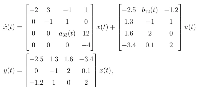
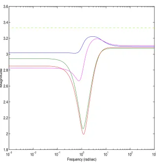
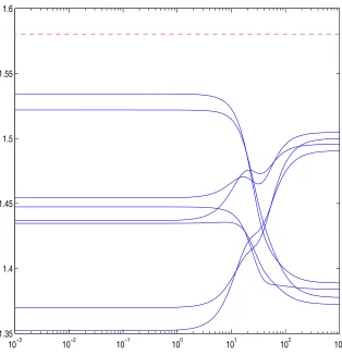
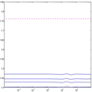
shown in Fig. 3.1. Alternatively, the model reduction problem has been solved using

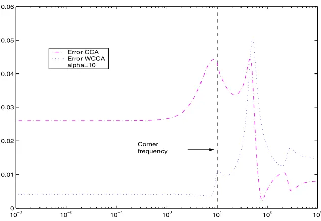
alternating projection method [40]. The sub-optimalγ level achieved is 3.79, which is slightly worse than the cone complementarity algorithm. The reduced-order models

and its upper bound is shown in figure 3.2. On the other hand, the computational

scheme based on cone complementarity algorithm is much faster than alternating

projection method. For this example both algorithms were computed in a Sun

Work-station Spark 10 and as we observed from the table the first method is over 20 times

10−3 10−2 10−1 100 101 102 103 1.8

2 2.2 2.4 2.6 2.8 3 3.2 3.4 3.6

Frequency (rad/sec)

Magnitude

102−3 10−2 10−1 100 101 102 103 2.2

2.4 2.6 2.8 3 3.2 3.4 3.6 3.8

Frequency (rad/s)

Magnitude

Some numerical experiments were performed comparing both methods. During

the study several random uncertain polytopic systems were created, modifying

char-acteristics such as number of states, desired reduced order and number of vertices.

The comparison between the two methods were oriented towards theγ level obtained which gives an idea of the fidelity of the approximation and the time needed for each

method as a measurement of the computational burden which becomes a serious issue

when working with large dimensional polytopes.

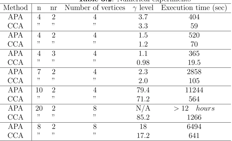
Table 3.2: Numerical experiments

Method n nr Number of vertices γ level Execution time (sec)

APA 4 2 4 3.7 404

CCA ” ” ” 3.3 59

APA 4 2 4 1.5 520

CCA ” ” ” 1.2 70

APA 4 3 4 1.1 365

CCA ” ” ” 0.98 19.5

APA 7 2 4 2.3 2858

CCA ” ” ” 2.0 105

APA 10 2 4 79.4 11244

CCA ” ” ” 71.2 564

APA 20 2 8 N/A >12 hours

CCA ” ” ” 85.2 1266

APA 8 2 8 18 6494

CCA ” ” ” 17.2 641

We can conclude clearly from the table that the CCA method performed

consid-erably better than the APA. In all the cases without exception the CCA was able to

find a smaller γ than the APA, which demonstrate that the reduced model obtained by the CCA is closer to the original system than the APA approximation. In terms

of computational effort, it is clear than the APA method is slower than CCA. In all

the cases studied the CCA algorithm was 20 times faster in average. In fact when

both methods were used to reduced a 20th _{order polytope with 4 vertices, after 12} hours has elapsed the APA method could converge to a satisfactory solution while

the CCA took only 21 minutes to obtain an approximation. This is evidence that the

3.6

Comparison Between CCA and Balanced

Truncation Method

In this section a brief description of the balanced truncation method is given and

finally a counter example is shown to demonstrate the inefficacy of this particular

method to deal with polytopic uncertain systems.

3.6.1

Description of the Balanced Truncation Method

Considers the problem of reducing the order of a linear multivariable dynamical

sys-tem using the balanced truncation method. Suppose

G(s) =    

A11 A12 B1

A21 A22 B2

C1 C2 D

  

∈ RH∞

is a balanced realization with controllability and observability gramians P = Q = Σ =diag(Σ1,Σ2) where

Σ1 =diag(σ1Is1, σ2Is2,· · · , σrIsr) (3.18) Σ2 =diag(σr+1Isr+1, σr+2Isr+2,· · · , σNIN) (3.19)

Then the truncated system G_r = 

 A11 B1

C1 D



 is stable and satisfies additive error

bound:

G(s)−G_r(s)_∞= N

i=r+1

σ_i, (3.20)

For a detailed explanation of this method and its extension to frequency weighted

model reduction, Chapter 7 of Zhou([21] offers and extensive description of the

math-ematical formulation as well as practical examples of the method applied to LTI

3.6.2

Counter Example

Since our objective is to approximate a polytopic uncertain linear system by a lower

order polytopic uncertain system with a guaranteed induced L2 norm error, a naive

approach to this problem would be to approximate each vertex separately using the

hankel balanced reduction method and then construct a reduced-order polytopic

un-certain system as a convex combination of the lower order vertices. It can be shown

easily by a counter-example that the reduced-order system obtained from this naive

approach may have an arbitrarily large approximation error.

To show the previous fact a random uncertain polytope of 8thorder and 8 vertices will be reduced, the system is defined as follows.

A(t) =            

−25 11 −5 5 5 1

−6 −32 −8 −6 −9 16 8 −13 −27 −1 0 10 2 −1 7 −29 −6 −16 −10 −3 −9 −1 −20 −1

13 −8 a63(t) 15 6 −32

           

, B(t) =             20 6

5 −6 19 6 −3 b42(t)

−11 1 −2 −20

            ,

C(t) =

−3 −6 −12 −1 9 −6 12 −23 11 4 c25(t) −7

, D=

12 0 −7 −8

.

where a63 ∈ [−9,−12] , b42 ∈ [−11,−9] and c25 ∈ [−21,−20]. We are interested

in second-order approximation, so the next step is to obtain a second order polytope

with the same number of vertices as the original system, this will be done using CCA

and Balanced truncation method. It is good to note that the reduce order polytope

obtained by balance truncation method, is the convex combination of the vertices

obtained by reducing each original vertex separately. As we denoted in section 3.1 a

measurement of the accuracy of the approximation will be given by

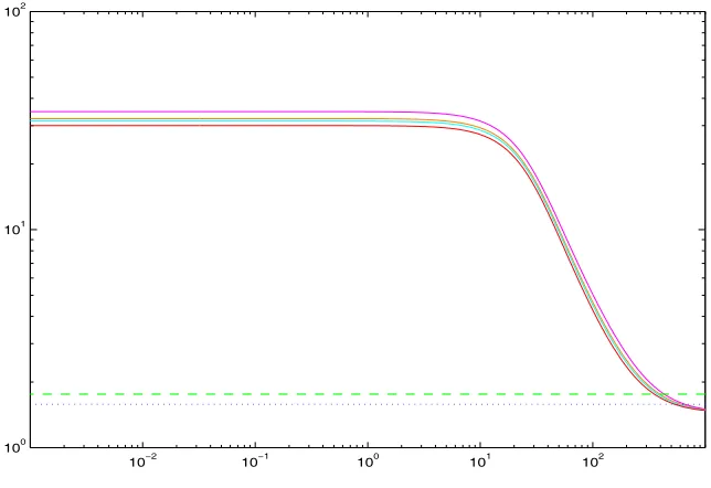
Now in figures 3.3 and 3.4 the error between each original vertex and its reduced

version is shown, for the approximation obtained trough CCA and Balanced

trun-cation respectively. In both figures the dashed line represent the upper bound that

each method guarantees.

10−3 10−2 10−1 100 101 102 103 1.35

1.4 1.45 1.5 1.55 1.6

10−2 10−1 100 101 102 1.4

1.45 1.5 1.55 1.6 1.65 1.7 1.75 1.8 1.85

Figure 3.4: The second order approximation errors at vertices using Balanced trun-cation method. The dashed line represent N_i=r+1σ_i

We seen that both methods provide valid results for the vertices and that the

error is below the predicted upper bound. Now the next step is obtained 4 random

systems that are elements of the previous polytope . To do this 4 vectors α∈ A are chosen randomly and then 4 systems denoted T_α1...Tα4 are obtained by the convex

combination of each α and all the 8 vertices. Now the corresponding error for the original and reduced system using both methods will be shown in figures 3.5 and 3.6

10−3 10−2 10−1 100 101 102 103 1.42

1.44 1.46 1.48 1.5 1.52 1.54 1.56 1.58 1.6

Figure 3.5: The second order approximation error for T_α1 . . .Tα4 using CCA, the

dashed line representsγr,2

10−2 10−1 100 101 102 100

101 102

Figure 3.6: The second order approximation error for T_α1 . . .Tα4 using APA, the

From the analysis of these plots we can conclude that the CCA accomplished its

objective, since the error is completely bounded byγr,2 _{for all the 4 random systems,}

which leads to the conclusion that the method guaranteed and bounded error not

only for the vertices, but for all the systems in the polytope.

On the other hand the Balanced truncation method provides a bounded error only

for the vertices (as seen in figure 3.4) but the error is completely unbounded for

all the random systems chosen in the polytope (see figure 3.6) it is clear that the

error is a lot bigger that the upper bound predicted by the Balanced method and

roughly speaking that implies a performance degradation of about 75% for this case,

something completely inadmissible, specially when the CCA error bound implies a

performance degradation of 3.5%.

Some partial conclusions can be drawn from the previous analysis made in this

chapter.

• First, compared with CCA and APA the Balanced truncation method is the fastest of the three, since its computational burden is very low

com-pared with the previous methods, but it can only handle LTI systems,

being completely inadequate for the reduction of polytopic uncertain

pa-rameter systems.

• And second, the CCA and APA methods are effective tools in the re-duction of polytopic uncertain parameter systems, but the comparison of

these two systems shows that the CCA reduces greatly the computational

load, which implies a faster execution and the ability to work with larger

dimensional uncertain systems.

• In terms of performance, the CCA seems consistently to obtain slightly better approximation than the APA, this can be seen in the error bound

Frequency Weighted Optimal

H

_∞

Model

Reduction Method

In this chapter we extend the previous model reduction scheme to frequency weighted

model reduction, an introductory background section is included to provide some

information about previous research done on the area, the second section outline the

problem definition and solvability conditions and finally and example is shown to

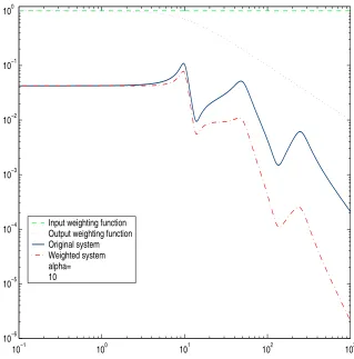
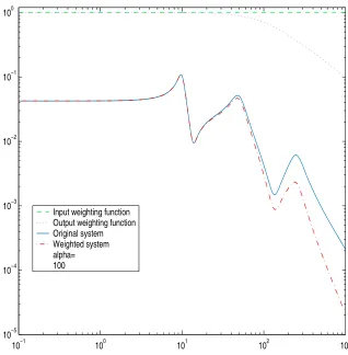
demonstrate how the approximation changes by changing the weighting functions.

4.1

Background

The motivation for a frequency weighted model reduction comes from the need to

cap-ture the approximation requirement over a pre-specified frequency range and desired

frequency bandwidth of input signals. Recently this area has received considerable

attention, the balanced truncation method was extended to frequency weighted case

by Enns [7]. Unfortunately, the stability of reduced-model was not guaranteed when

both input and output weights exist. Alternative approach to weighted balanced

truncation problem was proposed in [1] for a special class of weighting functions.

One side weighted model reduction problems with not necessarily stable weighting

functions [44] and self-weighted functions [45] were examined by Zhou using balanced

truncation techniques, and explicit error bounds were derived. For the extension of

optimal Hankel norm approximation to frequency weighted case, see e.g. [26],[14],

[45] and references therein. Note that these solutions are not necessarily optimal in

theH∞norm sense, hence variousH∞ norm lower and upper bounds of the weighted truncation errors were provided to quantify their sub-optimality.

This chapter considers frequency weighted model reduction problem for stable

linear uncertain polytopes systems and minimizesH∞ norm of the truncation errors. The result presented here is a generalization of the unweighted H_∞ model reduction scheme reported in ([16], [18]). Different from previous weighted model reduction

results, the reduced-order model is shown always stable while stable input and output

weighting functions involved and besides the method has been extended from LTI

systems to uncertain time varying parameter systems . A necessary and sufficient

optimality condition characterizing weighted H∞ model reduction problem is given in terms of LMIs with one extra rank constraint, which generally leads to a non-convex

problem. Again this non-convex constraint will be treated using CCA method, in the

same way we did with the unweighted case.

4.2

Problem Definition

Given a nth order polytopic uncertain linear system T ∈ G as defined in section 3.1 with input and output weighting function matrices W_i ∈ RHq×s_∞ , W_o ∈RHr×p_∞ , one wants to find an asymptotically stable,kth _{(k < n) order uncertain polytope T}r_{, such} that Tr is a good approximation of the original system T in the H_∞ norm sense. To be precise, consider the optimization problem

min Tr∈RHp∞×q

deg(Tr)≤k

where proper, stable transfer function matricesT, W_i, W_o have their state-space data as

T_p =ss 

 Ap Bp Cp _Dp



 f or p= 1. . . L (4.2)

where L represents the number of vertices. Note that we are going to use su-perscript p to denote the pth vertex, to avoid confusion with the subscripts _i and _o reserved for the input and output weighting functions respectively.

W_i =ss 

 Ai Bi C_i D_i



 W_o =ss 

 Ao Bo C_o D_o



 (4.3)

For the previous systems Ap _{∈ R}n×n_{, A}

i ∈ Rni×ni and Ao ∈ Rno×no. The eigen-values of Ap, A_i, A_o are in the open left-half plane for p = 1. . . L. Without lose of generality, it is assumed that

B_o D_o and

C_i D_i

have full column and row rank

respectively.

The following theorem is the main result and provides a sub-optimal solution to

the frequency weighted H∞ model reduction problem.

Theorem 3 Given γ > 0, the full order model T and weighting functions W_i, W_o

defined by (4.2). Let n_w := n+n_i +n_o, and

S_oT₁ S_oT_{2 T}

,

S_i1 Si2

_T

span the null

space of matrices

BT

o DTo

,

C_i D_i

respectively (that is, BT

oSo1+D_oTSo2 = 0 and

S_i1C_iT +Si2D_iT = 0). Define

ˆ Ap_w :=

   

Ap _{0 B}p_C

i 0 ST

o1Ao+SoT2Co 0

0 0 A_i

  

 A˜p_w :=    

Ap _{0 0}

B_oCp _A

o 0

0 0 A_iS_iT₁+B_iS_iT₂    

ˆ B_wpT :=

DT

i Bp T

0 BT i

_T

˜ C_wp :=

D_oCp _C o 0

f or p= 1. . . L.

Then the following statements are equivalent:

W_o(s)T_p(s)−T_pr(s)W_i(s)

∞< γ. f or p= 1. . . L.

2. There exist matrices X, Y ∈Snw×nw

+ , such that

          

I 0 0 0 ST

o1 0

0 0 I   

XAˆp_wT + ˆAp_wX    

I 0 0 0 S_o1 0

0 0 I    −γ    

0 0 0

0 ST

o2So2 0

0 0 0

    Bˆ_wp

ˆ

B_wpT −γI

       <0 (4.4)

f or p= 1. . . L           

I 0 0 0 I 0 0 0 S_i1

  

YA˜pw+ ˜Ap T w Y    

I 0 0 0 I 0 0 0 ST

i1    −γ    

0 0 0

0 0 0

0 0 S_i2S_iT2

    C˜wpT

˜ Cp

w −γI

       <0 (4.5)

f or p= 1. . . L

Y I

I X

≥0 (4.6)

rank

Y I I X

≤n_w+k. (4.7)

Furthermore, an asymptotically stable T_pr satisfying conditions (3.5)-(4.7) has its state-space data given by

Ar

p Brp C_pr D_pr

= (P2Q−221pP2T)− 1_(P